Formation and Collapse of Nonaxisymmetric Protostellar Cores in Planar Magnetic Molecular Clouds

Abstract

We extend our earlier work on ambipolar diffusion induced formation of protostellar cores in isothermal sheet-like magnetic interstellar clouds, by studying nonaxisymmetric collapse for the physically interesting regime of magnetically critical and supercritical model clouds ($\mu_{0}\geq 1$, where $\mu_{0}$ is the initial mass-to-magnetic flux ratio in units of the critical value for gravitational collapse). Cores that form in model simulations are effectively triaxial, with shapes that are typically closer to being oblate, rather than prolate. Infall velocities in the critical model ($\mu_{0}=1$) are subsonic; in contrast, a supercritical model ($\mu_{0}=2$) has extended supersonic infall that may be excluded by observations. For the magnetically critical model, ambipolar diffusion forms cores that are supercritical ($\mu_{\rm core}>1$) and embedded within subcritical envelopes ($\mu_{\rm env}<1$). Cores in our models have density profiles that eventually merge into a near-uniform background, which is suggestive of observed properties of cloud cores.

1 Introduction

Magnetic fields play an important role in star formation, especially in the early stages of core formation and collapse; measured mass-to-flux ratios of molecular clouds yield an average that is $\sim 1-2$ times greater than the critical value for collapse (Crutcher 1999). However, observational biases tend to push toward higher values of measured mass-to-flux ratio (Crutcher 2003, private communication), so that moderately subcritical cloud regions are not ruled out. Dense cores within molecular clouds are the sites of star formation, with detected infall up to $\approx 0.5\,c_{\rm s}\approx 0.1~{}\rm km~{}s^{-1}$ on scales $\lesssim 0.1~{}\rm pc$, (e.g., in L1544, Tafalla et al. 1998; Williams et al. 1999), where $c_{\rm s}$ is the isothermal sound speed. Ciolek & Basu (2000) have fit the main features of the observed velocity and density profiles in L1544, modeling it as an axisymmetric supercritical core embedded in a moderately subcritical envelope.

Axisymmetry is clearly an idealization to real cores. Observations suggest a typical projected axis ratio of 0.5 for cores (Myers et al. 1991), and deprojections of the distribution of shapes imply intrinsically triaxial but nearly oblate cores (Jones, Basu, & Dubinski 2001). Polarized emission measurements from dense cores also imply triaxiality (Basu 2000). More generally, detailed submillimeter maps of star-forming regions reveal significant irregular structure and multiple cores (Motte, André, & Neri 1998). Theoretical nonaxisymmetric magnetic models of the collapse and fragmentation of a single core were presented by Nakamura & Hanawa (1997) and Nakamura & Li (2002), without and with ambipolar diffusion, respectively, using the magnetic thin-disk approximation (Ciolek & Mouschovias 1993, hereafter CM93). The early stages of core formation in a nonaxisymmetric infinitesimally thin subcritical sheet (including the effects of magnetic tension but ignoring magnetic pressure) were studied by Indebetouw & Zweibel (2001). Here, we also study a planar cloud that is perpendicular to the mean magnetic field, focusing on the case of either exactly critical or decidedly supercritical cores; these cases are shown to lead to observationally distinguishable outcomes. We again use the thin-disk approximation, which allows for finite thickness effects, and explicitly includes the effects of both magnetic pressure and tension.

2 Physical and Numerical Model

The fundamental equations we use to model molecular clouds as self-gravitating, partially-ionized, isothermal thin sheets or disks have been presented in axisymmetric form in CM93 and Basu & Mouschovias (1994, hereafter BM94). In this study, the condition of axisymmetry is no longer employed, and instead we model clouds as thin sheets of infinite extent [with vertical half-thickness $Z(x,y,t)$] in a cartesian coordinate system ($x,y$). Magnetohydrostatic equilibrium in the $z$-direction (i.e., balance of thermal-pressure, gravitational, and magnetic pinching forces) is assumed at all times. The evolution is followed in a square region using periodic boundary conditions. To find the gravitational field components in the sheet, we calculate the gravitational potential $\psi(x,y,t)$. For this situation, solving Poisson’s equation (see eq. [29] of CM93) relates $\psi$ to the column density $\sigma_{\rm n}(x,y,t)$ ($=\int_{-Z}^{Z}\rho_{\rm n}(x,y,t)dz$; $\rho_{\rm n}$ is the mass density) by

$${\cal F}[\psi]=-2\pi G{{\cal F}[\sigma_{\rm n}]}/k_{z},$$ (1)

where ${\cal F}[f]$ is the Fourier transform of a function $f$, $k_{z}$ ($=[k_{x}^{2}+k_{y}^{2}]^{1/2}$) is the wavenumber, and $G$ is the gravitational constant. In our governing equations, the effects of magnetic pressure and magnetic tension are both included. The magnetic potential $\Psi(x,y,t)$ that is used to determine the $x$- and $y$- components of the magnetic field at the surface of the sheet (necessary to calculate magnetic tension forces) is also given by equation (1), by substituting $\psi$ with $\Psi$, and $2\pi G\sigma_{\rm n}$ with $-(B_{z,\rm eq}-B_{\rm ref})$; for details see CM93. $B_{z,\rm eq}(x,y,t)$ is the vertical magnetic field strength in the sheet, and $B_{\rm ref}$ is the uniform magnetic field of the background (reference) state, as well as the assumed constant magnetic field as $|z|\rightarrow\infty$. In the present study, we neglect magnetic braking due to a finite density external medium (BM94), and dust grains and UV ionization (CM93, Ciolek & Mouschovias 1995).

In our formulation, velocities are normalized to the isothermal speed of sound $c_{\rm s}=0.188\,(T/10~{}{\rm K})^{1/2}~{}\rm km~{}s^{-1}$ (where $T$ is the temperature and we have used a mean molecular mass $m=2.33m_{\rm H}$, in which $m_{\rm H}$ is the hydrogen atom mass), column densities are in units of $\sigma_{\rm n,0}$, the uniform column density of the background state. The time unit is $t_{0}=c_{\rm s}/2\pi G\sigma_{\rm n,0}$, the length unit is $L_{0}=c_{\rm s}^{2}/2\pi G\sigma_{\rm n,0}$, and the magnetic field unit is $B_{0}=2\pi G^{1/2}\sigma_{\rm n,0}$. As discussed in CM93 and BM94, model clouds are distinguished by three basic dimensionless parameters, namely, the initial mass-to-magnetic flux ratio (in units of the critical value for gravitational collapse) $\mu_{0}\equiv B_{0}/B_{\rm ref}=2\pi G^{1/2}\sigma_{\rm n,0}/B_{\rm ref}$, the initial dimensionless neutral-ion collision time $\tilde{\tau}_{\rm ni,0}\equiv\tau_{\rm ni}/t_{0}$, and the normalized external pressure acting on the disk, $\tilde{P}_{\rm ext}\equiv P_{\rm ext}/(\frac{\pi}{2}G\sigma_{\rm n,0}^{2})$. The ion number density $n_{\rm i}$ is calculated using the scaling law $n_{\rm i}\propto n_{\rm n}^{1/2}$ (as done by BM94; $n_{\rm n}$ is the neutral number density), which is a reasonable approximation for $n_{\rm n}\lesssim 10^{6}~{}{\rm cm}^{-3}$ (e.g., Ciolek & Mouschovias 1998). For a background number density $n_{\rm n,0}=3\times 10^{3}\,~{}{\rm cm}^{-3}$ and $\tilde{P}_{\rm ext}=0.1$, we find that $\sigma_{\rm n,0}=5.98\times 10^{-3}$ g cm^-2 (therefore $N_{\rm n,0}\equiv\sigma_{\rm n,0}/m=1.54\times 10^{21}~{}{\rm cm}^{-2}$), $L_{0}=4.57\times 10^{-2}$ pc, and $t_{0}=2.38\times 10^{5}$ yr.

We use the method of lines technique (e.g., Schiesser 1991); the system of partial differential equations of two-fluid MHD are converted to a system of ordinary differential equations (ODE’s) through second-order spatial finite differencing, and use of the van Leer (1977) advection scheme. Time integration of the ODE’s is performed using the implicit Adams-Bashforth-Moulton method. Details of our basic technique can be found in Morton, Mouschovias, & Ciolek (1994). Fast Fourier transform (FFT) routines are used to solve for the gravitational and magnetic potentials obtained through equation (1). The computational region has extent $4\lambda_{\rm T,m}$ on each side, where $\lambda_{\rm T,m}=4\pi L_{0}$ is the wavelength with maximum growth rate of gravitational instability in a non-magnetic (thermal) infinitesimally thin disk. Models presented in this paper are run on a uniform grid of $128\times 128$ points.

3 Results

We present the evolution of two model clouds; one model is exactly critical, with $\mu_{0}=1$, and the other is supercritical with $\mu_{0}=2$. Both models have $\tilde{\tau}_{\rm ni,0}=0.16$ (as adopted in the standard model of BM94) and $\tilde{P}_{\rm ext}=0.1$. Since the background (reference) state is characterized by a uniform column density $\sigma_{\rm n,0}$ and magnetic field $B_{\rm ref}\mbox{\boldmath$\hat{z}$}$ (where $B_{\rm ref}=B_{0}/\mu_{0}$) the gravitational and magnetic forces in the reference state are identically zero. To initiate evolution, we superimpose a set of random, small-amplitude (the rms is 3% of the background) column density perturbations $\delta\sigma_{\rm n}$. The magnetic field is also perturbed, with $\delta B_{z,\rm eq}\propto\delta\sigma_{\rm n}$, to maintain flux-freezing in the initial state of each model. The spectrum of perturbations is flat (white noise), with damping so that wavelengths of twice the grid spacing and smaller are negligible; we choose this particular type of spectrum so as not to preferentially excite modes with the maximum growth rate. The evolution of each model is followed until the maximum column density $\approx 10\,\sigma_{\rm n,0}$. Beyond this enhancement, gravitational instability cannot be spatially resolved, and the evolution is relatively very rapid in a small region near the density peaks, making a simulation of the larger cloud impractical even at higher resolution. Since the vertical balance along field lines is primarily between gas pressure $\rho_{\rm n}\,c_{\rm s}^{2}$ and self-gravitational pressure $\frac{\pi}{2}G\sigma_{\rm n}^{2}$, the density has increased by a factor $\approx 100$.

3.1 Critical model ($\mu_{0}=1$)

Figure 1 exhibits color images of the normalized column density $\sigma_{\rm n}(x,y)/\sigma_{\rm n,0}$ and the local mass-to-flux ratio $\mu(x,y)=2\pi G^{1/2}\sigma_{\rm n}/B_{z,\rm eq}$ over the entire computational region for the critical model at its final output time, $t=133.9\,t_{0}$. The time is rather long due to the very small-amplitude perturbations and because magnetic forces exactly balance gravity in the flux-freezing limit, requiring instability to be initiated by random ion-neutral drifts. Two major density peaks have formed by this time. The column density structure shows that the lowest density contours are the most irregular and elongated. Henceforth, we define a dense core to be the region within the $\sigma_{\rm n}/\sigma_{\rm n,0}=2$ contour, corresponding to the observationally significant threshold $n_{\rm n}\approx 10^{4}~{}{\rm cm}^{-3}$. The masses of the two dense cores in this simulation are $5.3M_{\odot}$ (lower left of Fig. $1a$) and $4.2M_{\odot}$ (upper right of Fig. $1a$), respectively, using the standard values of units given in § 2. For comparison, the enclosed mass in our periodic computational domain is $151M_{\odot}$. The shape of the cores are generally nonaxisymmetric, a result that was first seen in the magnetically subcritical planar ambipolar diffusion models of Indebetouw & Zweibel (2000). The mean value of $Z\equiv\sigma_{\rm n}/(2\rho_{\rm n})$ implies one oblate core with relative axis lengths 0.15:1:1, and another that is triaxial with relative lengths 0.1:0.7:1, making it more nearly oblate than prolate. The cores formed in this model always have their shortest axis aligned normal to the sheet (parallel to the mean magnetic field). Although one core is effectively oblate in this particular model realization, our simulations reveal they are most commonly triaxial and more nearly oblate than prolate, in accordance with statistical analyses of observed cores (Jones et al. 2001).

Velocity vectors of the neutrals are also displayed in Figure $1a$. Calculation of the rms speeds of neutrals ($v_{\rm n,rms}$) and ions ($v_{\rm i,rms}$) in the entire computational region yield $v_{\rm n,rms}=0.114\,c_{\rm s}=1.14\,v_{\rm i,rms}$; ions lag behind neutrals because the motions are ultimately gravitationally driven. Furthermore, all of the infall speeds in this model are subsonic. The maximum infall speed is $|v_{\rm n}|=0.54\,c_{\rm s}$, and speeds of this order occur only within the cores. As we shall see in § 3.2, subsonic infall is a distinct feature of ambipolar-diffusion initiated collapse in clouds with $\mu_{0}\lesssim 1$. This trend is consistent with multi-line studies that find subsonic gas speeds in dense protostellar cores (Tafalla et al. 1998; Williams et al. 1999), and with axisymmetric models of core formation in subcritical clouds (Ciolek & Basu 2000).

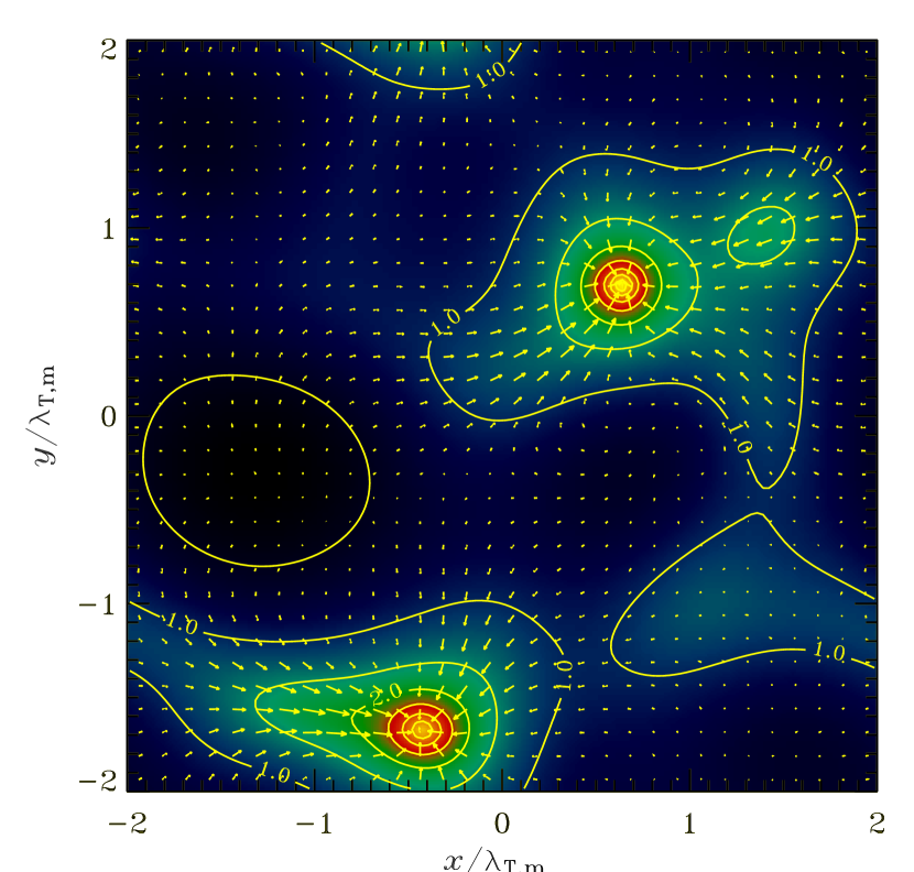
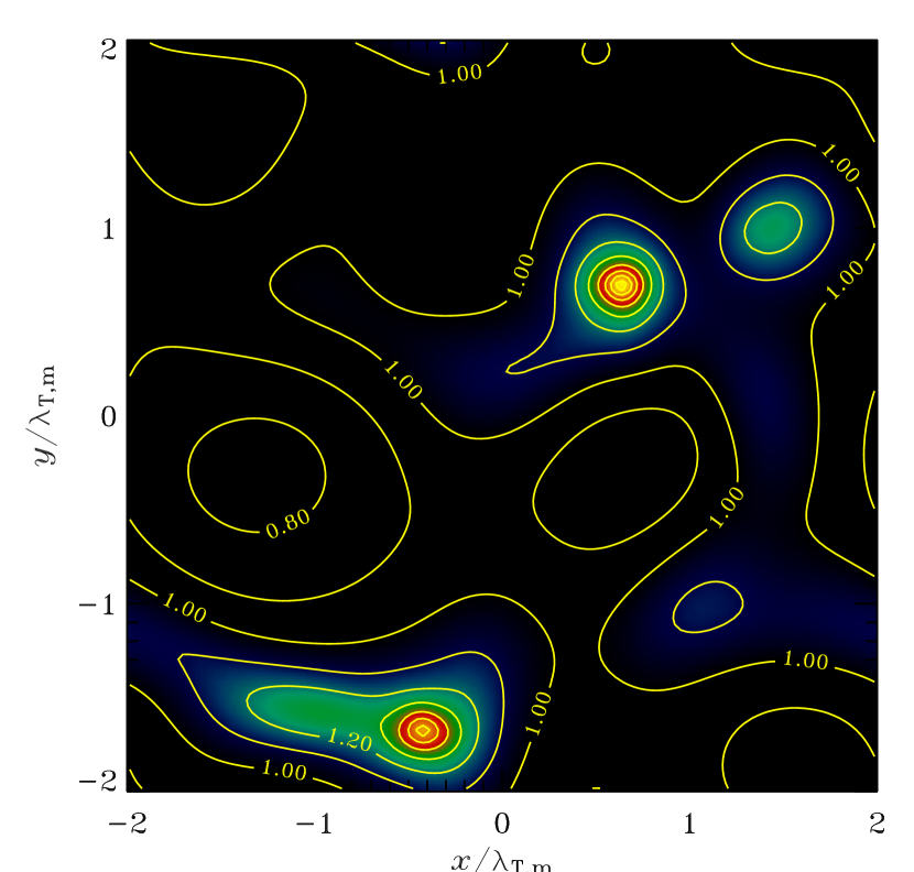
Figure 1: Critical model ($\mu_{0}=1$). The data are shown when the maximum column density $\approx 10\,\sigma_{\rm n,0}$. (a, Left.) Image and contour plot of normalized column density $\sigma_{\rm n}(x,y)/\sigma_{\rm n,0}$. The contour lines are spaced in multiplicative increments of $2^{1/2}$. Also shown are velocity vectors of the neutrals; the distance between tips of vectors corresponds to a speed $0.5\,c_{\rm s}$. (b, Right.) Image and contours of $\mu(x,y)$, the mass-to-flux ratio in units of the critical value for collapse. Regions with $\mu<1$ are black. The contour lines are spaced in additive increments of 0.1.

Figure $1b$ shows another interesting result: the cores are supercritical ($\mu_{\rm core}>1$) and are surrounded by magnetically subcritical envelopes ($\mu_{\rm env}<1$). This is a natural consequence of ambipolar diffusion, which redistributes mass in magnetic flux tubes (Mouschovias 1978). Due to the initial precise balance between gravitational and magnetic forces in this model, evolution occurs as ambipolar diffusion effects a drift of mass through essentially stationary magnetic field lines. In time, this leads to the formation of both supercritical cores and a subcritical envelope. This can also occur in clouds with $\mu_{0}$ slightly above unity.

Figure 2 shows the column density $\sigma_{\rm n}/\sigma_{\rm n,0}$, vertical magnetic field $B_{z,\rm eq}/B_{0}$, and $x$-component of neutral velocity $v_{{\rm n},x}/c_{\rm s}$ along the $x$-axis for a line that cuts through one of the cores shown in Figure 1. The core stands out as a well-defined high density region with an eventual merger into a lower-density background (the remnant of the initial uniform state) that surrounds it; this is reminiscent of the mid-infrared absorption maps of dense cores made by Bacmann et al. (2000). The magnitude of $v_{{\rm n},x}$ increases inward toward the core center (but remains subsonic throughout) before dropping to zero at the core center.

Figure 2: Physical quantities in the $\mu_{0}=1$ model, along a line parallel to the $x$-axis that cuts through a supercritical core (shown in Figure 1) centered at $x=0.64\,\lambda_{\rm T,m},y=0.70\,\lambda_{\rm T,m}$. Solid curve: column density $\sigma_{\rm n}/\sigma_{\rm n,0}$. Dashed curve: magnetic field strength $B_{z,\rm eq}/B_{0}$. Dotted curve: $x$-component of the neutral velocity, $v_{{\rm n},x}/c_{\rm s}$.

3.2 Supercritical model ($\mu_{0}=2$)

Figure $3a$ exhibits a color image and contour plot of $\sigma_{\rm n}/\sigma_{\rm n,0}$, as well as velocity vectors for the supercritical model at its final output time, $t=17.6\,t_{0}$. The time is significantly lesser than in the previous model due to the relative ease of gravitational instability in a supercritical cloud. Because the evolution is more rapid and dynamical in the supercritical model, ambipolar diffusion doesn’t have as much time to operate. Hence, the mass-to-flux ratios of the high-density cores in this model ($\mu_{\rm core}\simeq 2.1$) are only slightly greater than the initial value. The core shapes are again nonaxisymmetric, either near-oblate or decidedly triaxial. For this model we find $v_{\rm n,rms}=0.222\,c_{\rm s}=1.05\,v_{\rm i,rms}$; these results differ from the critical model due to the more dynamical evolution and greater ability of neutrals to drag ions and magnetic field with them. The maximum infall speed is $1.19\,c_{\rm s}$, and speeds of this order typically occur within distances $\approx 0.1$ pc from the core centers. In contrast to the critical model, the infall speeds within the cores in this model are often supersonic, and significant motions $\approx 0.5\,c_{\rm s}$ are also seen throughout the cloud, and well outside the cores. Figure $3b$ shows $\sigma_{\rm n}/\sigma_{\rm n,0}$, $B_{z,\rm eq}/B_{0}$, and $v_{{\rm n},x}/c_{\rm s}$ along the $x$-axis for a line passing through one of the cores in Figure $3a$. The collapsing core again has a density profile that eventually merges into the background.

Our model shows that the extent of the supersonic flow region is well within the resolution capability of current observations (scales $\lesssim 0.1~{}{\rm pc}$, $n_{\rm n}\approx 10^{4}-10^{5}~{}{\rm cm}^{-3}$). Since supersonic infall has not been detected over these length scales and densities, and models with $\mu_{0}\gtrsim 2$ would have even greater infall speeds, this suggests that molecular clouds that are supercritical by a factor $\gtrsim 2$ are incompatible with observations of protostellar cores.

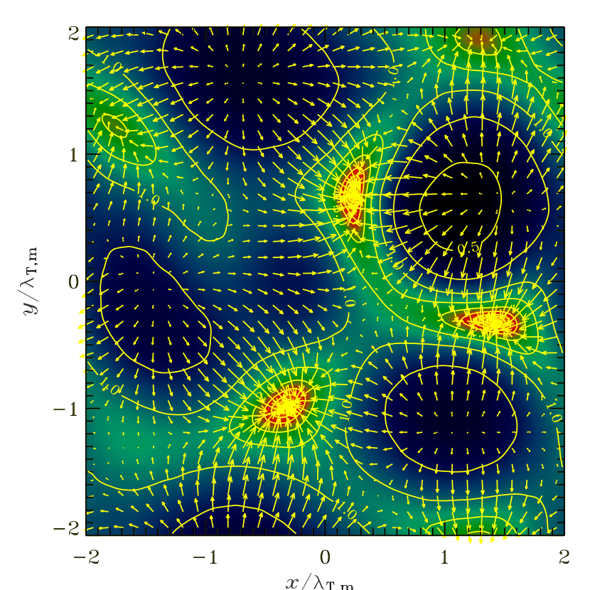
Figure 3: Supercritical model ($\mu_{0}=2$). The data are shown when the maximum column density $\approx 10\,\sigma_{\rm n,0}$. (a, Left.) Image and contour plot of normalized column density $\sigma_{\rm n}(x,y)/\sigma_{\rm n,0}$. The contour lines are spaced in multiplicative increments of $2^{1/2}$. Also shown are velocity vectors of the neutrals; they are normalized in the same way as in Fig. $1a$. (b, Right.) Physical quantities along a line parallel to the $x$-axis that cuts through a supercritical core centered at $x=1.42\,\lambda_{\rm T,m},y=-0.33\,\lambda_{\rm T,m}$. Solid curve: column density $\sigma_{\rm n}/\sigma_{\rm n,0}$. Dashed curve: magnetic field strength $B_{z,\rm eq}/B_{0}$. Dotted curve: $x$-component of the neutral velocity, $v_{{\rm n},x}/c_{\rm s}$.

4 Conclusions

Ambipolar diffusion leads to a nonuniform distribution of mass-to-flux ratio, in a natural extension of the process described by Mouschovias (1978). Stars form preferentially in the most supercritical regions. Core shapes are somewhat triaxial, and usually more nearly oblate than prolate. The core column density eventually merges into a near-uniform background value. In the critical ($\mu_{0}=1$) model, a surrounding region is established which is mildly magnetically subcritical (due to flux redistribution) and infall motions both inside and outside cores are subsonic. Conversely, the supercritical ($\mu_{0}=2$) model exhibits supersonic motions within cores, and extended rapid motions outside them. The critical model requires a significantly longer time to develop gravitational instability; however, we caution that the growth time for both models are likely upper limits due to the possibility of nonlinear perturbations in more realistic situations. We also note that all motions in these models are fundamentally gravitationally driven; the neutral speeds are typically greater than those of the ions.

References

- (1) Bacmann, A., André, P., Puget, J.-L., Abergel, A., Bontemps, S., & Ward-Thompson, D. 2000, A&A, 361, 555
- (2) Basu, S. 2000, ApJ, 540, L103
- (3) Basu, S., & Mouschovias, T. Ch. 1994, ApJ, 432, 720 (BM94)
- (4) Ciolek, G. E., & Basu, S. 2000, ApJ, 529, 925
- (5) Ciolek, G. E., & Mouschovias, T. Ch. 1993, ApJ, 454, 194 (CM93)
- (6) Ciolek, G. E., & Mouschovias, T. Ch. 1995, ApJ, 418, 774
- (7) Ciolek, G. E., & Mouschovias, T. Ch. 1998, ApJ, 504, 280
- (8) Crutcher, R. M. 1999, ApJ, 520, 706
- (9) Indebetouw, R., & Zweibel, E. G. 2000, ApJ, 532, 361
- (10) Jones, C. E., Basu, S., & Dubinski, J. 2001, ApJ, 551, 387
- (11) Morton, S. A., Mouschovias, T. Ch., & Ciolek, G. E. 1994, ApJ, 421, 561
- (12) Motte, F., André, P., & Neri, R. 1998, A&A, 336, 150
- (13) Mouschovias, T. Ch. 1978, in Protostars & Planets, ed. T. Gehrels (Tucson: Univ. Arizona), 209
- (14) Myers, P. C., Fuller, G. A., Goodman, A. A., & Benson, P. J. 1991, ApJ, 376, 561
- (15) Nakamura, F., & Hanawa, T. 1997, ApJ, 480, 701
- (16) Nakamura, F., & Li, Z.-Y. 2002, ApJ, 566, L101
- (17) Schiesser, W. E. 1991, The Numerical Method of Lines: Method of Integration of Partial Differential Equations (San Diego: Academic)
- (18) Tafalla, M., Mardones, D., Myers, P. C., Caselli, P., Bachiller, R., & Benson, P. J. 1998, ApJ, 504, 900
- (19) van Leer, B. 1977, JCP, 23, 276
- (20) Williams, J. P., Myers, P. C., Wilner, D. J., & DiFrancesco, J. 1999, ApJ, 513, L61