A Preliminary Observational Search for Circumbinary Disks Around Cataclysmic Variables

Abstract

Circumbinary (CB) disks have been proposed as a mechanism to extract orbital angular momentum from cataclysmic variables (CVs) during their evolution. As proposed by Taam & Spruit, these disks extend outwards to several a.u. and should be detected observationally via their infrared flux or by absorption lines in the ultraviolet spectra of the CV. We have made use of archival HST/STIS spectra as well as our own near-IR imaging to search for observational evidence of such CB disks in seven CVs. Based on the null result, we place an upper limit on the column density of the disk of ${N_{\rm H}}\sim 10^{17}{\rm\,cm}^{-2}$.

1 INTRODUCTION

Cataclysmic variables (CVs) are mass transferring binary star systems consisting of a white dwarf primary star and red dwarf secondary star. The evolutionary path from detached binary star system to close, interacting binary star system is greatly affected by orbital angular momentum loss (OAML), of which there must be significant amounts in order to transform the originally long period progenitor into an interacting binary (see Howell et al., 2001). A large amount of the OAML occurs during the common envelope (CE) phase of the CV evolution.

Although the exact mechanism for OAML is still a matter of debate, several theories have been advanced to explain the observed orbital period-mass transfer distribution of CVs. Generally, magnetic braking is invoked for long period systems ($P_{\rm orb}>3$ hr), and although these models are marginally successful in explaining the observed distributions, they predict a strong correlation between mass transfer rate ($\dot{M}$) and orbital period, along with an excessive number of ultra-short period, very low luminosity systems; neither the stringent $\dot{M}-P_{\rm orb}$ correlation, nor the preponderance of low luminosity systems are observed. The discord between theory and observation could be due to a number of different factors, the most intriguing of which is that magnetic braking may not be solely responsible for OAML, but rather angular momentum may be extracted from the binary system via a circumbinary (CB) disk (Spruit & Taam, 2001; Taam & Spruit, 2001; Dubus et al., 2002; Taam, Sandquist, & Dubus, 2003). The gravitational torque exerted by the CB disk on the binary will cause significant OAML leading to an accelerated period evolution and allowing the secondary star to completely dissolve within a finite time (less than a Hubble time). These two consequences are the attraction of the CB disk theory, as they would cause a broad range of $\dot{M}$ for any given period and remove the need for a large population of faint CVs.

If CB disks exist, they likely begin formation during the CE phase and acquire material via mass outflow from the white dwarf (novae) or accretion disk (winds and outbursts) (Spruit & Taam, 2001). For the CB disk to become a significant source of OAML, the mass input rate into the CB disk must be $10^{-5}$ to 0.01 of the material transferred from the secondary to the white dwarf throughout the CB disk lifetime. CB disks are assumed to be geometrically thin with a pressure scale height to radius ratio of $H/R\sim 0.03$, have a viscosity $\alpha\lesssim 0.01$, and of Keplerian structure. Dubus et al. (2002) have proposed that the inner edge is truncated due to tidal forces from the binary, has a radius near $1\times 10^{11}{\rm\,cm}$, effective temperature $T\sim 3000$ K, and is optically thick, while the majority of the outer disk is cool, $T<1000$ K, optically thin, and can extend out to several a.u. Continuum contribution comes from dust emission, with opacities due to dust grains, and includes contributions from iron-poor opacities at $T\lesssim 1500$ K where dust particles exist. Based on models of protoplanetary disks (e.g., Bell et al., 1997), Dubus et al. (2002) find that their CB disks reach a maximum vertical height above the plane of the disk at a radius less than the outer edge of the disk. However, the exact physical height of the outer edge of the CB disk is not known (R. Taam, private communication). Figure 1 shows a schematic model of a CB disk based on specifications given in Dubus et al. (2002).

Two properties of the proposed CB disks will manifest observationally; the large extent of the CB disk and its surface mass density, $\Sigma\sim 10^{2}-10^{4}\,{\rm g}{\rm\,cm}^{-2}$, should make the disk a source of ”ISM-like” absorption lines appearing at the systemic velocity of the system, and, if the CB disk emission (from the warm inner edge) can be considered to be a sum of blackbodies, the flux from the CB disk will peak near $3\,\micron$ (Dubus et al., 2002). These properties lend themselves to detection in two different wavelength regions. Flux measurements via near-IR ($1-10\,\micron$) imaging of face-on systems (offering a full view of the CB disk) may detect the IR flux of the CB disk. A second detection technique is to search for the ISM-like absorption lines produced by the CB disk in UV spectra of the binary systems. Hubble Space Telescope/ Space Telescope Imaging Spectrograph (HST/STIS) data are ideal for this as the high spectral resolution will enable detection and measurement of ISM-like lines whose radial velocities may then be compared to the space motion of the binary. This technique is best done for CVs with inclinations that match the opening angle of the CB disk, as the binary is then observed through the plane of the CB disk. The theoretical work (e.g., Taam & Spruit, 2001) predicts that the higher mass transfer rate CVs are the best candidates for a CB disk, as material may continuously be entering the CB disk, and may still retain some vertical extent above the disk (i.e., the CB disk has not had time to “flatten out”). Thus, we have begun an observational search for CB disks with long period nova-likes and old novae.

2 FEASIBILITY OF CB DISK DETECTION

While we have chosen CV candidates that should be ideal for detecting the proposed CB disks, the feasibility of disk detection depends quite a bit on the unknown CB disk structure. Here we discuss four different models for the disk structure - isothermal, isentropic, constant density scale height, and constant pressure scale height - and their significance for detecting a CB disk via their absorption signatures.

2.1 Key Assumptions

The CB disk is expected to extend for several orders of magnitude in barycentric distance, $R$, from the binary (Spruit & Taam, 2001). The dependence of the vertically-integrated surface mass density, $\Sigma$, on radius, $R$, is taken from Taam & Spruit (2001), particularly Figure 8 in that paper, from which we approximate

$$\Sigma=\Sigma_{\rm in}\left({R\over R_{\rm in}}\right)^{-1}.$$ (1)

Here $\Sigma_{\rm in}=10^{4}{\rm\,g\,cm^{-2}}$, and $R$ extends from $R_{\rm in}$ to $R_{\rm out}$, which we take to be $10^{11}\,{\rm cm}$ and $10^{14}\,{\rm cm}$, respectively (Dubus et al., 2002). Unlike a Shakura-Sunyaev disk, the opening angle, $H/R$, is expected to be roughly constant. We choose $H/R=\theta_{\rm open}\simeq 0.03\simeq 1.7^{\circ}$, taken from Figure 2 of Dubus et al. (2002).

This value for $\theta_{\rm open}$, as well as the relation for $\Sigma$ in eq. (1), are assumed to be the same for each CV system. The difference between each system is then contained wholly in the inclination, $i$, or equivalently, the parameter $\theta_{\rm view}$, the viewing angle, where $90^{\circ}-i=\theta_{\rm view}$. Note that the smallest viewing angle in our sample occurs with EX Hya, where $\theta_{\rm view}=12^{\circ}\pm 1^{\circ}$, which corresponds to a height above the midplane of roughly $z/H\sim 7$, where $z=R\sin\theta_{\rm view}\simeq R\theta_{\rm view}$ is the height above the disk.

2.2 Vertical Disk Profile

In order to estimate the density above the midplane, we need a model for the vertical density profile of the disk. If we are within one pressure scale height of the midplane, then the uncertainty in the density is relatively small, but the theoretical uncertainty becomes much greater for higher $|z|$. Various processes, such as turbulent transport, transport by sound waves, and so forth, affect the vertical entropy profile, which in turn determines the vertical density profile. In hot disks, there is the further potential complication of winds being driven off the disk or a hot corona. Even in relatively cool disks there may also be photoevaporation off the disk by the illumination from the central binary. We leave these considerations to future theoretical work on the subject of CB disks.

In calculating a vertical density profile for a disk, it is standard to assume a plane-parallel atmosphere. Note that in this case there is a vertical gravity in the disk that increases linearly with $z$:

$$g_{\rm eff}=\left({GM_{\rm binary}\over R^{3}}\right)z=\Omega_{K}^{2}z,$$ (2)

where $\Omega_{K}$ is the Keplerian angular velocity, so that the equation of vertical hydrostatic equilibrium is

$$\partial_{z}P=-\rho\Omega_{K}^{2}z.$$ (3)

This equation can not be solved without some additional physics to inform us of the vertical entropy profile, such as the local heating rate, $q+$, due to turbulent dissipation, and the radiative and turbulent transport of energy out of the disk. Some insight into this problem is provided by theoretical work (e.g., Cassen, 1993), but uncertainties remain, especially at altitudes of several scale heights.

First let us comment on the disk thickness (or half-thickness), $H$. From a disk theorist’s perspective, $H$ is usually taken to be a rough quantity that comes about in basic mixing-length-theory arguments. Given a location in the disk, $H$ is determined by the sound speed, which in turn is determined by the temperature. All of this is tied together by standard thin-disk theory, in which quantities are taken to be functions of $R$ only, so that the vertical structure appears only through some rather rough approximations.

It is common to refer to this $H$ as “the” pressure scale height, but when considering the vertical structure in greater detail, this definition is no longer sufficient. The local vertical pressure scale height, $h_{P}$, defined as $h_{P}^{-1}=-(\partial_{z}P)/P$, may vary significantly with height, $z$, above the midplane; in fact it becomes formally infinite at the midplane. So, from the operational standpoint of an observer, there may be some significant ambiguity in defining $H$, which we need to address. While there have been theoretical studies of the vertical density profile for certain disks, we are not aware of any theoretical treatment of the vertical density profile for CB disks that extends to several scale heights above the midplane. What we offer here is a few simple models for the disk structure. Hopefully future theoretical and observational work will further constrain these models.

Mathematically, one option for defining $H$ is that it is the normalized second moment of the density,

$$\Sigma H_{1}^{2}=\int_{-\infty}^{+\infty}\rho z^{2}\,dz.$$ (4)

An alternative definition of $H$ that is perhaps of more use to the observer is in terms of the photospheric surface $\tau=2/3$. We also note that Bell et al. (1997) define $H$ in terms of the “midplane pressure scale height”, $c_{s}/\Omega$. For the isothermal disk and the isentropic disk, we take $H=H_{1}$ as defined above, and for the constant density scale height and (modified) constant pressure scale height models, we take $H$ to be equal to the local density and pressure scale heights, respectively.

2.3 Model A: Isothermal Disk Atmosphere

For a disk that is vertically isothermal, at a given radius, $R$, we have $\rho\sim P$. The equation of hydrostatic equilibrium, eq. (2), then gives $\partial_{z}\rho\sim-\rho z$, which has solution $\rho=\rho_{0}\exp{(-az^{2})}$. The local pressure scale height is $h_{P}^{-1}=2az$. If we set $h_{P}=z=H$, we find $2aH^{2}=1$, so that

$$\rho=\rho_{0}\exp{(-z^{2}/2H^{2})}.$$ (5)

It is easy to verify that the $H$ in this solution coincides with the definition for $H_{1}$ given above, so setting $h_{P}=z=H$ is appropriate. Note that the local pressure scale height $h_{P}$ (which in this case is also the local density scale height) is then

$$h_{P}={H^{2}\over|z|},$$ (6)

i.e., it diverges at the midplane, is equal to $H$ at $z=\pm H$, and asymptotes to zero at infinity.

The corresponding surface density, $\Sigma$, for this solution is

$$\Sigma=\int_{-\infty}^{+\infty}\rho(z)\,dz=\sqrt{2\pi}\rho_{0}H.$$ (7)

In terms of $\Sigma$ and the height above the disk, $z$, the density becomes

$$\rho={\Sigma\over H\sqrt{2\pi}}\exp{(-z^{2}/2H^{2})}.$$ (8)

2.4 Model B: Isentropic Disk Atmosphere

For an isentropic disk, we begin with the equation of state $P=A\rho^{\gamma}$, where $A\equiv{P_{0}/\rho_{0}^{\gamma}}$, and $P_{0}$ and $\rho_{0}$ are fiducial values of the pressure and density, respectively, taken at the midplane. From equation (3) we have that

$${d\rho\over\rho^{2-\gamma}}=-{\Omega_{\rm K}^{2}\over\gamma A}z\,dz,$$ (9)

which may be integrated to find

$$\rho=\rho_{0}\left[1-\left({z\over z_{\rm max}}\right)^{2}\right]^{1\over\gamma-1}.$$ (10)

A very notable aspect of this solution is that $\rho=0$ for $|z|>z_{\rm max}$ for some $z_{\rm max}$. Note that $z_{\rm max}$ may be written as a function of $A$, $\Omega_{\rm K}$, and $\gamma$, although we do not reproduce the solution here. Assuming that $\gamma=5/3$, we find that

$$\Sigma={3\over 8}\pi\rho_{0}z_{\rm max}.$$ (11)

We wish to know the $H$ that corresponds to the above solution. Here the matter is not so simple as for the isothermal case, and we must take care to define $H$ appropriately, as discussed above. In the case of $H$ defined in terms of the normalized second moment of the density, i.e., $H_{1}$, we find

$$H_{1}={z_{\rm max}\over\sqrt{6}}\simeq(2.50)^{-1}z_{\rm max},$$ (12)

so that, if we set $H=H_{1}$, we may now write

$$\rho={\Sigma\over H}{8\over 3\pi\sqrt{6}}\left[1-\left({z\over H\sqrt{6}}\right)^{2}\right]^{3/2}$$ (13)

for $|z|<H\sqrt{6}$, and $\rho=0$ otherwise.

2.5 Model C: Constant Density Scale Height Disk Atmosphere

The constant density scale height disk is rather trivial. If we define $H$ as the local density scale height,

$$h_{\rho}^{-1}=-{\partial_{z}\rho\over\rho}=H,$$ (14)

we find that

$$\rho={\Sigma\over 2H}\exp{(-|z|/H)}.$$ (15)

2.6 Model D: Constant Pressure Scale Height Atmosphere with Isothermal Core

The constant pressure scale height atmosphere would seem to be an attractive model. However, it presents an unphysical solution. Namely, if we set

$$h_{P}^{-1}=-{\partial_{z}P\over P}=H,$$ (16)

we find through equation (3) that

$$\rho\sim{H\over|z|}\exp{(-|z|/H)},$$ (17)

so that that density diverges at the midplane, and moreover the vertical integral of the density, i.e., $\Sigma$, diverges as well.

As an alternative, we consider here an isothermal vertical profile near the midplane (the “core”), with a constant pressure scale height solution “glued” onto the isothermal solution at $|z|=H$. This has the somewhat unsatisfactory result that the vertical derivative of the density is discontinuous at $|z|=H$, i.e., there is a “kink” in the solution, but this way the divergence mentioned above is avoided. We then have

$$\rho_{|z|<H}=\rho_{0}\exp{(-z^{2}/2H^{2})}$$ (18)

and

$$\rho_{|z|>H}=\rho_{0}e^{1/2}{H\over|z|}\exp{(-|z|/H)}$$ (19)

where $\rho_{0}$ is determined by the error function and the exponential integral, yielding the numerical value

$$\rho_{0}\simeq(0.4107){\Sigma\over H}.$$ (20)

We may then write

$$\rho_{|z|<H}=(0.4107){\Sigma\over H}\exp{(-z^{2}/2H^{2})}$$ (21)

and

$$\rho_{|z|>H}=(0.6773){\Sigma\over H}{H\over|z|}\exp{(-|z|/H)}.$$ (22)

2.7 Column Densities for the Models

It is important to note that, in all cases, the solution $\rho(\Sigma,H,z)$ may be written in the form

$$\rho(\Sigma,H,z)={\Sigma\over H}f(|z|/H)$$ (23)

for some function $f()$.

The column number density of hydrogen, ${N_{\rm H}}$, is

$${N_{\rm H}}=\int n_{\rm H}\,d\ell$$ (24)

where $d\ell$ is an infinitesimal displacement along the line of sight to the binary. We assume here that the hydrogen mass fraction of the disk is near unity, so that $n_{\rm H}\simeq\rho/m_{\rm H}$.

In peforming the integral, the key assumptions are: a constant flare angle $H/R$ with radius $R$, the expression given above in eq. (1) for the dependence of $\Sigma$ upon radius, and the functional form in eq. (23) for the density. Furthermore, we assume that the density drops immediately to zero when $R$ is outside the range $(R_{\rm in},R_{\rm out})$. Note that $d\ell=\sec{\theta_{\rm view}}\,dR\approx dR$. We therefore have

$${N_{\rm H}}={1\over m_{\rm H}}\int_{R_{\rm in}}^{R_{\rm out}}\rho(\Sigma,R,z)\,dR$$ (25)

The argument of $f()$ that appears in the expression for $\rho$ in eq. (23), namely $|z|/H$, is a constant, equal to $\tan\theta_{\rm view}/\tan\theta_{\rm open}\approx\theta_{\rm view}/\theta_{\rm open}$. The choice of $\Sigma\sim R^{-1}$ is rather fortuituous from the point of view of performing this integral. Given that $R_{\rm out}\gg R_{\rm in}$ and using the small-angle approximation, we find

$${N_{\rm H}}={1\over m_{\rm H}}{f(\eta)\over\theta_{\rm open}}\Sigma_{\rm in}.$$ (26)

where $\eta\equiv\theta_{\rm view}/\theta_{\rm open}$.

The numerical value of the column density for our four models may then be written as follows. For Model A, the isothermal model,

$${N_{\rm H}}=(8.03\times 10^{27})\left({\Sigma_{\rm in}\over 10^{4}{\rm\,g\,cm^{-2}}}\right)\left({\theta_{\rm open}\over 1.7^{\circ}}\right)^{-1}\exp{\left(-\frac{\eta^{2}}{2}\right)},$$ (27)

For Model B, the isentropic model, we find

$${N_{\rm H}}=(6.98\times 10^{27})\left({\Sigma_{\rm in}\over 10^{4}{\rm\,g\,cm^{-2}}}\right)\left({\theta_{\rm open}\over 1.7^{\circ}}\right)^{-1}\left(1-\frac{\eta^{2}}{6}\right)^{3/2}.$$ (28)

For Model C, the constant density scale height atmosphere,

$${N_{\rm H}}=(1.01\times 10^{28})\left({\Sigma_{\rm in}\over 10^{4}{\rm\,g\,cm^{-2}}}\right)\left({\theta_{\rm open}\over 1.7^{\circ}}\right)^{-1}\exp{(-|\eta|)},$$ (29)

and for the constant pressure scale height atmosphere with isothermal core,

$${N_{\rm H}}=(8.27\times 10^{27})\left({\Sigma_{\rm in}\over 10^{4}{\rm\,g\,cm^{-2}}}\right)\left({\theta_{\rm open}\over 1.7^{\circ}}\right)^{-1}\exp{\left(-\frac{\eta^{2}}{2}\right)}\,\,\,\,{\rm for}\,\,\,\,|\eta|<1$$ (30)

$${N_{\rm H}}=(1.36\times 10^{28})\left({\Sigma_{\rm in}\over 10^{4}{\rm\,g\,cm^{-2}}}\right)\left({\theta_{\rm open}\over 1.7^{\circ}}\right)^{-1}\left(\frac{1}{|\eta|}\right)\,\exp{(-|\eta|)}\,\,\,\,{\rm for}\,\,\,\,|\eta|>1.$$ (31)

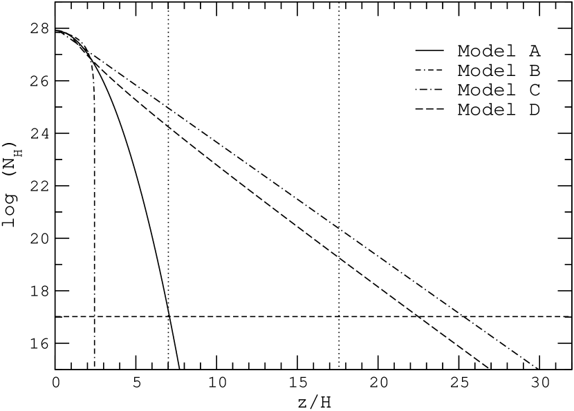
Figure 2 displays these values as functions of $z/H(=\theta_{\rm view}/\theta_{\rm open})$.

2.8 Discussion of the Solutions

As may be seen in Figure 2, the expected density profile for small values of $|z|/H$ ($|z|<2H$) does not depend too much upon the model chosen. Essentially, $\rho$ is expected to be of the order of $\Sigma/H$, dropping gradually as $|z|$ increases, and this is what is seen.

The situation changes quite dramatically, however, when we consider much larger $|z|$, as can be seen in Figure 2. As discussed above, the density in the adiabatic solution drops to zero at roughly $|z|/H\simeq 2.50$, for $\gamma=5/3$ and $H=H_{1}$. The density remains rather high in the two constant scale height solutions, dropping exponentially or close to exponentially depending upon whether it is the density scale height or the pressure scale height that is kept constant. The isothermal solution is a sort of compromise between these extremes, dropping as a Gaussian. It is unlikely that a CB disk with a structure described by Model B would be detectable in any CV system that does not have $i\sim 90^{\circ}$. CB disks with structures described by models A, C, and D, however, would be detectable in systems with lower inclinations.

3 OBSERVATIONS

As this project is an initial investigation for CB disks around CVs, we chose to look at a concise sample of objects that met our criteria: bright, high mass transfer systems (including the old nova, DI Lac); known inclinations and systemic velocities; and existing HST/STIS spectra that would be retrievable via the Multimission Archive at Space Telescope (MAST). The six objects we chose for spectroscopic investigation are listed in Table A Preliminary Observational Search for Circumbinary Disks Around Cataclysmic Variables and the data sets utilized are given in Table 2. Each HST/STIS observation employed the E140M grating in Echelle mode, which spans the wavelength range $1150-1735$Å, and has a resolving power of $R=45,800$, or $\sim 0.02$ Å pixel^-1 throughout each spectrum. The data were retrieved from the MAST archive and processed using IRAF/STSDAS software. We used IRAF/SPLOT to analyze the spectra.

Four of the spectra are of excellent quality: IX Vel and V3885 Sgr both have a signal-to-noise ratio of $\sim 30$ in the continuum, and QU Car and EX Hya have $S/N\sim 20$ in the continua. The spectra of DI Lac and TZ Per are slighty noisier, with signal-to-noise ratios of 5 and 10, respectively. The DI Lac spectrum is too noisy shortward of $1200$Å to properly identify any spectral features below this wavelength.

We also present near-IR $JHKL^{\prime}$ band photometric data of the nova-like CV, V592 Cassiopeia. V592 Cas was observed in $JHK$ at the Wyoming Infrared Observatory (WIRO) in 1997 (Ciardi et al., 1998) and in $L^{\prime}$ at the Fred Lawrence Whipple Observatory 1.2 m telescope on Mt. Hopkins for a total of 5 minutes on 1999 January 1 UT. The $JHKL^{\prime}$ data were obtained as part of a campaign to study IR properties of CV secondaries. Additional $JHK$ observations of V592 Cas have been secured at the United Kingdom IR Telescope on Mauna Kea and are in agreement with the WIRO data.

4 ANALYSIS AND DISCUSSION

For each spectrum, we identified absorption lines of ionic species commonly associated with the ISM and CV systems, such as C, N, Mg, Si, and S. We considered absorption lines that are above the $2\sigma$ error level in flux and that have full width at half maximum (FWHM) values $<0.2$ Å, as absorption lines with larger FWHM values would not be associated with the slowly rotating CB disk or the ISM. Absorption lines were fit with a single Gaussian function to determine line centers and equivalent widths (EWs). Some absorption lines are composed of well-separated multiple absorption components (for example, the absorption lines of QU Car); for these we measured the line centers of the components individually. At the resolution of the E140M grating, our spectra are not sufficient to resolve closely spaced ISM features; for absorption lines containing unresolvable components, we measured the lines with a single Gaussian. Radial velocities for all measured absorption components were then calculated and are given in Table 3, along with the EWs of the absorption lines. The measurement errors on the radial velocities for narrow lines that are unblended and unsaturated are within the velocity resolution of the spectrum, which is typically $\sim 3{\rm\,km\,s^{-1}}$. Lines with EW $\,>100$ mÅ are likely saturated or close blends of two strong components. In such circumstances, it is difficult to assign a meaningful centroid velocity to these features; we therefore assign uncertainties of $\pm 7{\rm\,km\,s^{-1}}$ to the radial velocities calculated for these lines. Absorption lines of excited state ions are noted in the table by an asterisk.

4.1 ISM Lines of Sight

Many of the identified absorption lines will be due to absorption by the ISM, in particular the local interstellar cloud (LIC); the warm, partially ionized cloud in which the Sun resides. The heliocentric velocity of the LIC is $25.7{\rm\,km\,s^{-1}}$ towards the Galactic coordinates $l=186\fdg 1$, $b=-16\fdg 4$ (e.g., Wood et al., 2002). Evidence of the LIC is frequently observed over a large fraction of the sky as a distinct range of velocities associated with ISM absorption components present in high dispersion UV spectra of nearby stars (e.g., Lallement & Bertin, 1992; Holberg, Barstow, & Sion, 1998; Wood et al., 2002; Kimura, Mann, & Jessberger, 2003). In addition to the LIC, many other velocity components are also observed in certain directions. The LIC and these other components are commonly discussed in terms of an assemblage of warm interstellar clouds within 30 pc of the sun. A good up-to-date and lucid description of these ISM velocity components is provided in Frisch, Grodnicki, & Welty (2002, hereafter FGW). In Table A Preliminary Observational Search for Circumbinary Disks Around Cataclysmic Variables, we give the velocity of the LIC in the direction of each of our candidate objects.

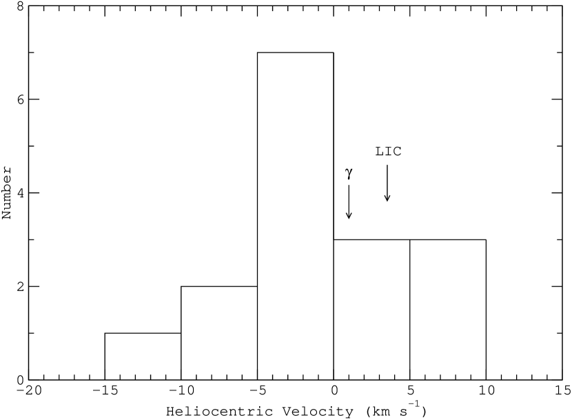
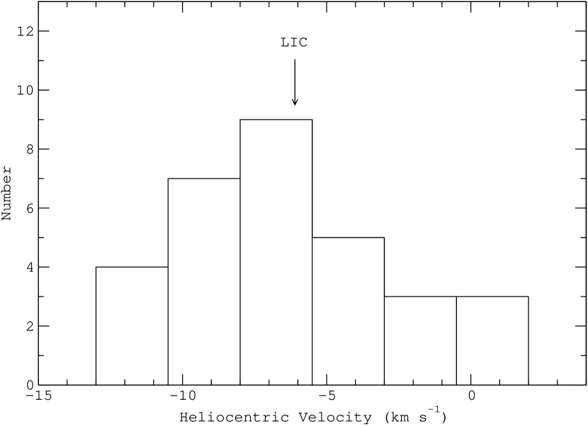
The LIC velocity is easily recognized in the histograms we have created for the ISM-like absorption lines found in the spectra of the six CV systems we studied. These histograms are shown in Figures 3 - 8. For four of the six objects, DI Lac, IX Vel, TZ Per, and QU Car, the LIC velocity is at or near the peak velocity in the histograms. EX Hya and V3885 Sgr do not follow suit; the peak in the EX Hya histogram is $\sim 7{\rm\,km\,s^{-1}}$ from the LIC velocity, and neither of the peaks in the V3885 Sgr histogram are aligned with the LIC velocity.

The line of sight to DI Lac lies in a direction expected to show LIC components. However, the projected LIC velocity very nearly coincides with the systemic velocity of the system, making it difficult to observationally distinguish either (see Figure 3). Complicating matters is the presence of lines due to interstellar C I, an ion not present in the LIC because it is easily destroyed by the ambient stellar UV radiation field. The presence of C I lines indicates that the line of sight to DI Lac passes through a diffuse cloud with sufficient density to preserve the C I ion. The presence of an unusually dense component of the ISM is also indicated by the very strong and saturated lines of S II. The mean velocity of the C I lines and the S II lines ($-1.78{\rm\,km\,s^{-1}}$) contributes significantly to the peak in the velocity distribution adjacent to the predicted LIC velocity. It would be tempting to associate these lines with a CB disk, however, the velocities are not consistent and the physical conditions in the CB disk are not appropriate to the existence of the C I ion. Rather, it appears that the line of sight to DI Lac passes through a relatively dense interstellar cloud, unrelated to the CV system. There is no evidence in the spectrum of DI Lac of lines arising from a CB disk.

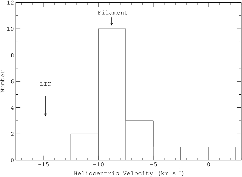
The line of sight to EX Hya lies in a direction that shows no LIC components. The peak of the radial velocity histogram (Figure 4) does, however, coincide with the expected velocity of the Filament structure described in FGW, consistent with several stars that lie in the same general direction as EX Hya. There is no evidence for a CB disk and the line of sight to this star is consistent with the ISM only.

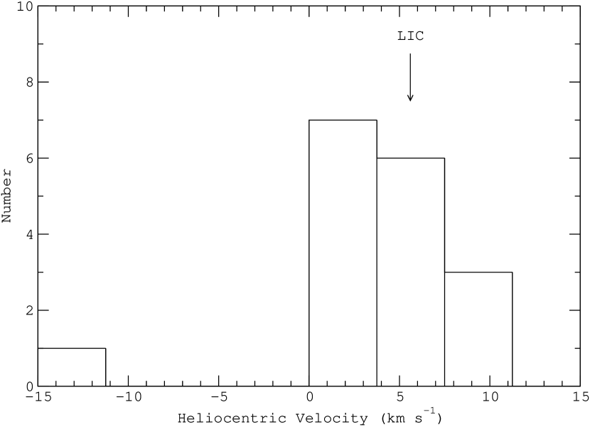
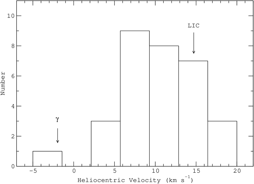
For IX Vel and QU Car, the line of sight to each object lies in a direction expected to show LIC components and the peaks of the histograms coincide with the expected LIC velocity (see Figures 5 and 6). The line of sight to IX Vel is consistent with the ISM only. The spectrum of QU Car shows several relatively weak C I lines, indicating the line of sight passes through a relatively dense interstellar cloud. There is no indication of CB disk related absorption for QU Car.

The line of sight to TZ Per lies in a direction expected to show LIC components, however, the histogram of velocities (see Figure 7) shows a broad distribution of velocities. Like the spectrum of DI Lac, the spectrum of TZ Per contains C I lines as well as relatively strong S II lines, consequently a similar interpretation - a line of sight through a dense interstellar cloud - holds for TZ Per. Many of the features in the TZ Per spectrum are either saturated or quite strong, indicating that several unresolved velocity components are present and contributing to the broad distribution of velocities. There is one C I line appearing near the systemic velocity, however, this is not sufficient evidence to support absorption from a CB disk and as discussed above, the existence of this ion in a CB disk is not probable.

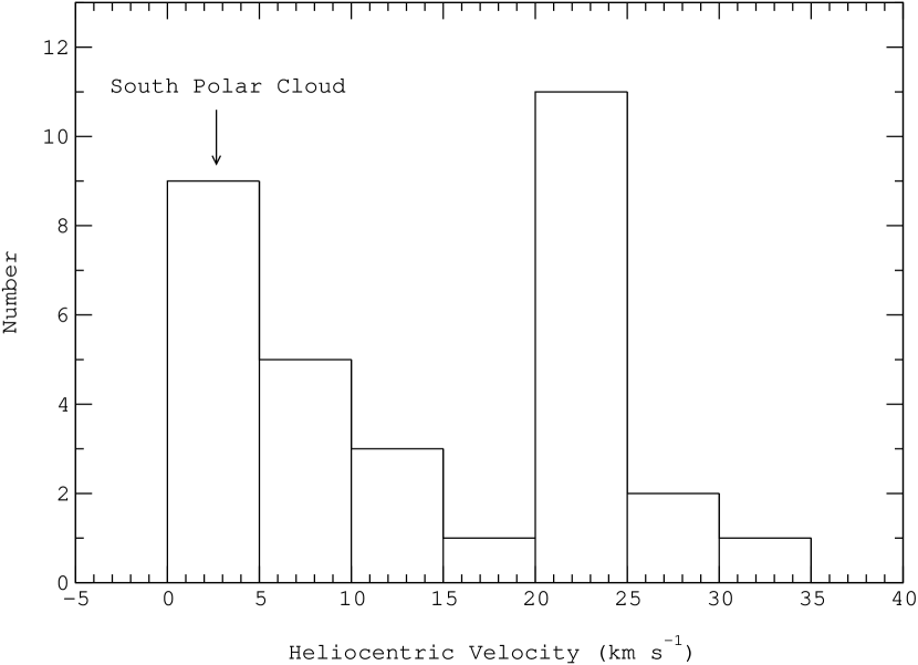
The line of sight to V3885 Sgr contains two distinct, well separated velocity components (see Figure 8). The component at $+2.5{\rm\,km\,s^{-1}}$ can be confidently identified with the South Polar Cloud (see FGW). The second peak near $20{\rm\,km\,s^{-1}}$ corresponds to no previously described interstellar cloud in the local ISM. There is no clear contribution from the LIC or a CB disk. The line of sight to this star is consistent with the ISM only.

4.2 Absorption Line Velocities

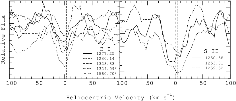
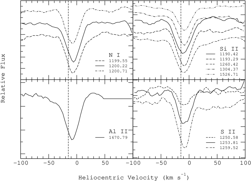
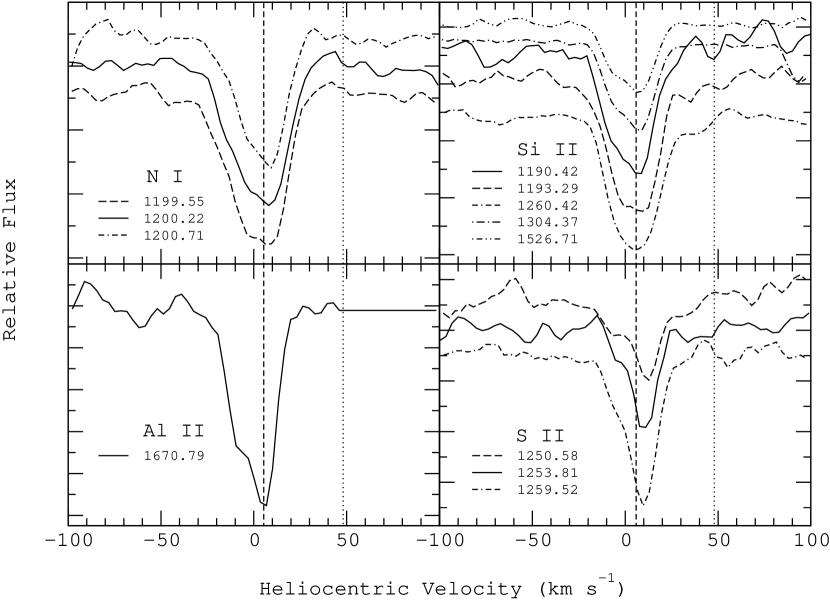
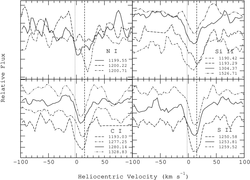
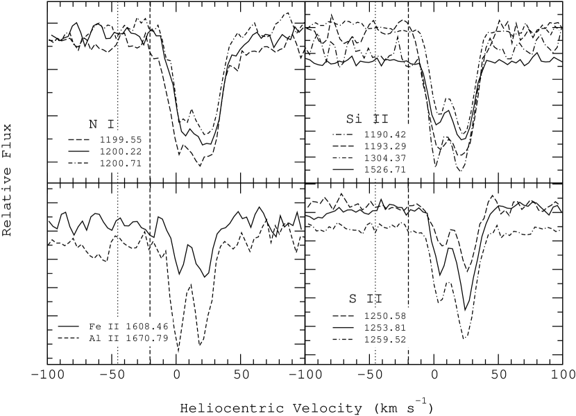
Figures 9 - 14 display line velocity profiles for select absorption lines from the spectra of each of the six CVs. On each plot, the vertical dashed line represents the LIC velocity towards the object, and the vertical dotted line represents the systemic velocity of the system. For systems that have systemic velocities with large errors, the dotted line represents the measured value. We selected a sampling of absorption lines to illustrate the line structure and velocity behavior for each system. Shown are the common absorption lines of the N I $\lambda\lambda 1199.55,1200.22,1200.71$ triplet, lines from several C I multiplets, the S II $\lambda\lambda 1250.58,1253.81,1259.52$ triplet, lines from several Si II multiplets, along with the Fe II $\lambda 1608.46$ and Al II $\lambda 1670.79$ absorption lines (excited transitions are noted with an asterisk).

Figure 9 displays absorption lines found in the spectrum of DI Lac. Each line exhibits a single velocity structure, however, because the LIC velocity and systemic velocity are separated by less than the velocity resolution of the spectrum, it is not possible to identify the absorption lines with either velocity. As discussed in the previous section and based on the results from the remaining objects of our study (see below) it is likely that the absorption lines in the DI Lac spectrum are ISM in nature. The 1910 nova eruption of DI Lac implies the presence of nova shells, which may be observed via absorption lines, however, these lines should be blue-shifted with respect to the systemic velocity.

The absorption lines found in the EX Hya spectrum (shown in Figure 10) have a single velocity structure. They are shifted $\sim 7-10{\rm\,km\,s^{-1}}$ with respect to the LIC velocity of $-14.8{\rm\,km\,s^{-1}}$, but are aligned with the Filament structure discussed in FGW. The line velocities of IX Vel (Figure 11) and QU Car (Figure 12) are aligned with the LIC velocity. In each case, the systemic velocity of the system is clearly not associated with the absorption line velocities.

TZ Per (Figure 13) is another system for which the LIC and systemic velocities fall within the velocity width of the absorption line profiles. The two velocities are separated by more than the velocity resolution of the spectrum, therefore the absorption line velocities may be identified with the LIC velocity, as it is more closely aligned with the absorption line centers (the LIC velocity alignment is also seen in Figure 7).

The absorption lines in the V3885 Sgr spectrum (Figure 14) have two velocity components; one that is aligned with the South Polar Cloud (FGW) and one that does not match any known ISM velocity system. Sagittarius is in the direction of the galactic center, so it is likely that different clouds along this line of sight are causing absorption along the line of sight to V3885 Sgr.

4.3 Infrared Observations

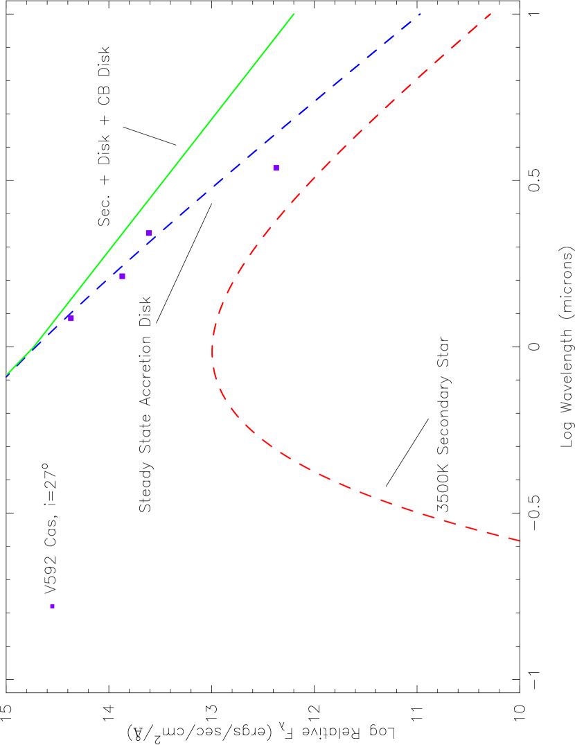
Although the outer regions of the proposed CB disks are cool and optically thin and not a source of IR blackbody flux, the warm, optically thick inner regions of the disk will make a contribution to the IR flux of a CV system. Given that the inner region of the CB disk is predicted to have a temperature of up to $\sim 3000$ K and is optically thick, we approximated a mean temperature of the CB disk that agrees well with Figure 2 of Dubus et al. (2002) to create a blackbody model representative of the CB disk. Determining this temperature is important, as the peak of the blackbody curve of the CB disk should cause an observable ’bump’ in the spectral energy distribution (SED) of the CV.

V592 Cas has an inclination of $i=27\arcdeg$, and is therefore ideal for detecting the full CB disk via IR observations. In Figure 15, we plot $JHKL^{\prime}$ points for V592 Cas, along with blackbody curves representing the secondary star for the system and a steady state accretion disk. Also plotted is the sum of the IR flux from all components of the CV system, including the flux contribution expected from a CB disk; it is a sum of blackbodies and peaks near $3\,\micron$. This model summed spectrum overestimates the IR flux observed for V592 Cas; the data points do not fall along the model curve that includes the flux contribution of the CB disk, but rather follow the blackbody curve of the steady state accretion disk. It is apparent that flux from a CB disk is not evident in the IR data of V592 Cas.

4.4 Observations of the ISM

Most of the spectral features observed in the six CV systems studied can be reasonably assigned to the LIC or other recognized velocity structures in the local ISM near the Sun. However, in several CVs (DI Lac, QU Car, and TZ Per), we do observe unusually strong lines due to S II and features due to C I, indicating that the line of sight to these stars passes through a dense, warm ISM component where C I is shielded from ionizing radiation. It is regarded as unlikely that these regions are associated with either CB disks or other gas related to the CV, as the observed velocities of these components are distinctly different from the CV system velocity.

4.5 Evidence for CB Disks?

In the spectroscopic and photometric data presented here, we have found no convincing evidence to support the theory of CB disks around CVs. The ISM-like lines appearing in the spectra of the six CVs have velocities consistent with the ISM in the direction of the object. The two cases in which the systemic velocity fell within the velocity width of the measured absorption lines (DI Lac and TZ Per) were complicated by the fact that the systemic velocity was close to the LIC velocity and that the identified lines were unlikely to occur in a CB disk. Based on the results of the other four objects, the match of the systemic velocity is due purely to its proximity to the LIC velocity. Evidence for a CB disk was not found in the $JHKL^{\prime}$ photometric data of V592 Cas. There is no excess of flux around the expected peak wavelength of $3~{}\micron$, and models of a CB disk overestimate the flux measured in V592 Cas.

In the absence of any absorption features clearly associated with CB disks, the upper limits for the disk material may be derived based on 3$\sigma$ upper limits for the EWs of N I, Si II, O I, and S II, evaluated at the systemic velocity in the spectrum of each CV (except for DI Lac, which exhibits some lines near the systemic velocity). The 3$\sigma$ EW values for all lines measured are very low - they range between 5 mÅ - 25 mÅ - so we can use the linear portion of the curve of growth to determine the species column densities: $N_{i}=1.129\times 10^{20}(\frac{W_{i}}{\lambda_{i}})(\frac{1}{f_{i}\lambda_{i}})$. Wavelengths and $f$ values are taken from Morton (1991). To calculate equivalent H column densities, we use typical abundances of each species observed for the warm phase of the ISM, $A_{i}$, such that ${N_{\rm H}}=\frac{N_{i}}{A_{i}}$. The best upper limits we calculate are from the N I and O I lines. For EX Hya we determine a value of ${N_{\rm H}}\sim 3\times 10^{17}{\rm\,cm}^{-2}$, for IX Vel $N_{\rm H}\sim 1\times 10^{17}{\rm\,cm}^{-2}$, for QU Car ${N_{\rm H}}\sim 2\times 10^{17}{\rm\,cm}^{-2}$, for TZ Per ${N_{\rm H}}\sim 2\times 10^{17}{\rm\,cm}^{-2}$, and for V3885 Sgr ${N_{\rm H}}\sim 2\times 10^{17}{\rm\,cm}^{-2}$.

We have indicated the observational upper limit of ${N_{\rm H}}\sim 10^{17}{\rm\,cm}^{-2}$ as the dashed horizontal line in Figure 2 for comparison of the observational numerical values with the theoretical disk models. The vertical dotted line at $z/H\sim 7$ represents the value of $z/H$ for EX Hya, while the vertical dotted line at $z/H\sim 17$ represents the value of $z/H$ for IX Vel, QU Car, and V3885 Sgr (the values for DI Lac and V592 Cas are past the limits of the plot). If CB disks exist, we can eliminate Models C and D as the proposed CB disk structure for the four CVs, as the model column densities are significantly above the detection limit and absorption by such disk structures would be detectable at the given inclinations. A CB disk with the structure of Model A would be detectable for the inclination of EX Hya and can therefore be ruled out, as no absorption from a CB disk is seen in EX Hya. Model B would not be observed in any of our CV systems, but we note that this model is the most conservative disk assumption of the four and we do not expect it to be physically realistic (i.e., we would expect the CB disk to have some form of an atmosphere).

As this investigation has only considered a small sample of CV systems that could contain a CB disk, we plan to continue our photometric and spectroscopic investigation for CB disks. In particular, we plan to analyze additional archival STIS data and to continue to look for their signatures in the IR SEDs of candidate CVs.

Figure 1: A schematic of a CV orbital plane showing the inner edge of a model CB disk. The inner disk starts near $10^{11}$ cm, is warm and optically thick. The outer edge is cold, optically thin, and extends out to several A.U.

Figure 2: Vertical density profiles above the CB disk midplane for disk structure models A, B, C, and D. The vertical dotted line at $z/H=7$ represents the value for EX Hya, while the line at $z/H=17$ represents the z/H value for IX Vel, QU Car, and V3885 Sgr. The horizontal dashed line at $\log{N_{\rm H}}=17$ represents the $3\sigma$ upper limit for the column densities, based on measurements of the HST spectra (discussed in a later section).

Figure 3: Histogram of the radial velocities of ISM-like absorption lines measured in the spectrum of DI Lac. Labeled are the systemic ($\gamma$) and calculated LIC velocities, neither of which match the peak velocity in the histogram.

Figure 4: Histogram of the radial velocities of ISM-like absorption lines found in the spectrum of EX Hya. The LIC velocity is labeled at $-15{\rm\,km\,s^{-1}}$, while the velocity of the Filament structure discussed in FGW at $-9{\rm\,km\,s^{-1}}$ is also labeled.

Figure 5: Histogram of the radial velocities of ISM-like absorption lines found in the spectrum of IX Vel. The peak of the histogram matches well with the LIC velocity of $5.6{\rm\,km\,s^{-1}}$.

Figure 6: Histogram of the radial velocities of ISM-like absorption lines found in the spectrum of QU Car. The peak velocity of the histogram corresponds to the LIC velocity of $-6.1{\rm\,km\,s^{-1}}$.

Figure 7: Histogram of the radial velocities of ISM-like absorption lines found in the spectrum of TZ Per. There is a grouping of lines with velocities around $5-15{\rm\,km\,s^{-1}}$ - the LIC velocity falls at the high end of this range. One absorption line has a velocity that matches the systemic velocity (labeled as $\gamma$) at $-2{\rm\,km\,s^{-1}}$.

Figure 8: Histogram of the radial velocities of ISM-like absorption lines found in the spectrum of V3885 Sgr. The two peaks in the histogram, at $\sim 4{\rm\,km\,s^{-1}}$ and $\sim 22{\rm\,km\,s^{-1}}$, represent the two velocity components of the absorption lines. The peak at $\sim 4{\rm\,km\,s^{-1}}$ matches well with the South Polar Cloud.

Figure 9: Line velocity profiles for absorption lines from four C I multiplets and the S II triplet observed in the DI Lac spectrum ($S/N\sim 5$). The dashed line at $3.5{\rm\,km\,s^{-1}}$ represents the LIC velocity, while the dotted line at $1{\rm\,km\,s^{-1}}$ represents the systemic velocity.

Figure 10: Line velocity profiles for the N I triplet, lines from several Si II multiplets, the Al II$\lambda 1670$ line, and the S II triplet found in the EX Hya spectrum ($S/N\sim 20$). The dashed line at $-14.8{\rm\,km\,s^{-1}}$ represents the LIC velocity.

Figure 11: Line velocity profiles for the N I triplet, lines from several Si II multiplets, the Al II$\lambda 1670$ line, and the S II triplet found in the IX Vel spectrum ($S/N\sim 30$). The dashed line at $5.6{\rm\,km\,s^{-1}}$ represents the LIC velocity, while the dotted line at $48{\rm\,km\,s^{-1}}$ represents the systemic velocity. The velocity centers of the absorption lines clearly match the calculated LIC velocity.

Figure 12: Line velocity profiles for the N I triplet, lines from several Si II and C I multiplets, and the S II triplet appearing in the QU Car spectrum ($S/N\sim 20$). The dashed line at $-6.1{\rm\,km\,s^{-1}}$ represents the LIC velocity, while the dotted line at $-84{\rm\,km\,s^{-1}}$ represents the systemic velocity. The velocity line centers are in good agreement with the calculated LIC velocity.

Figure 13: Line velocity profiles for the N I triplet, lines from several Si II and C I multiplets, and the S II triplet appearing in the TZ Per spectrum ($S/N\sim 10$). The dashed line at $14.7{\rm\,km\,s^{-1}}$ represents the LIC velocity, while the dotted line at $-2{\rm\,km\,s^{-1}}$ represents the systemic velocity. Both the systemic and LIC velocities fall within the velocity widths of the absorption lines, but it is the LIC velocity that most closely matches the line centers.

Figure 14: Line velocity profiles for the N I triplet, lines from several Si II multiplets, the Fe II $\lambda 1608$ and Al II$\lambda 1670$ lines, and the S II triplet appearing in the V3885 Sgr spectrum ($S/N\sim 30$). The dashed line at $-20.0{\rm\,km\,s^{-1}}$ represents the LIC velocity, while the dashed line at $-45{\rm\,km\,s^{-1}}$ represents the systemic velocity. Each absorption line exhibits a two velocity component structure.

Figure 15: A blackbody model of the IR flux of V592 Cas, including the contribution from a CB disk, created using a steady state CV accretion disk code. The model for the CB disk is a “sum of blackbodies” and the flux peaks near $3\,\micron$. Also plotted are the $JHKL^{\prime}$ data points for V592 Cas, which do not match the CB disk blackbody curve.

Table 1: Object Log

	$l$, $b$	Inclination ($z/H$)	LIC Velocity	Distance	Systemic Velocity
Object (type )	(deg)	(deg)	(${\rm\,km\,s^{-1}}$)	(pc)	(${\rm\,km\,s^{-1}}$)	References
DI Lac (N)	$103.107$, $-4.855$	$18$ (42)	+0$3.5$	$2500$	$1$	1,2
EX Hya (IP)	$303.186$, $33.622$	$78\pm 1$ (7)	$-14.8$	$64.5\pm 1.2$	$-180$	3,4
IX Vel (NL)	$264.929$, $-7.890$	$60\pm 5$ (17.6)	+0$5.6$	$95\pm 12$	$48$	5,6
QU Car (NL)	$293.513$, $-7.717$	$60$ (17.6)	$-6.1$	$2000$	$-84\pm 20$	7,8
TZ Per (DN)	$133.576$, $-2.777$	$\cdots$	$14.7$	$80$	$-2\pm 2$	9,10
V3885 Sgr (DN)	$357.477$, $-27.762$	$50-70$ (17.6)	$-20.0$	$110\pm 25$	$-45\pm 4$	5,11,12
V592 Cas (NL)	$118.603$, $-6.910$	$28\pm 11$ (36)	+0$9.9$	$60$	$21\pm 14$	13

References. — (1) Moyer et al. (2003); (2) Kraft (1964); (3) Hellier et al. (1987); (4) Beuermann et al. (2003); (5) Beuermann & Thomas (1990); (6) Perryman et al. (1997); (7) Gilliland & Phillips (1982); (8) Drew et al. (2003); (9) Echevarría et al. (1999); (10) Berriman, Szkody, & Capps (1985); (11) Cowley et al. (1977); (12) Haug & Drechsel (1985); (13) Huber et al. (1998)

Table 2: HST Observations Log

				Exposure Time
Object	Data Set	Observation Date	Grating	(s)	S/N
DI Lac	O5B607010	2000 April 19	E140M	2127	5
EX Hya	O68301010	2000 May	E140M	15,200	20
IX Vel	O5BI01010	2000 April 3	E140M	1750	30
QU Car	O5BI08010	2000 July 21	E140M	2600	20
TZ Per	O5B610010	2000 July 3	E140M	2151	10
V3885 Sgr	O5BI04010	2000 April 30	E140M	2480	30

Table 3: Identified Absorption Lines

		DI Lac		EX Hya		IX Vel		QU Car		TZ Per		V3885 Sgr
Ion $\lambda_{\rm rest}$		RV	EW	RV	EW	RV	EW	RV	EW	RV	EW	RV	EW
(Å)		(${\rm\,km\,s^{-1}}$)	(mÅ)	(${\rm\,km\,s^{-1}}$)	(mÅ)	(${\rm\,km\,s^{-1}}$)	(mÅ)	(${\rm\,km\,s^{-1}}$)	(mÅ)	(${\rm\,km\,s^{-1}}$)	(mÅ)	(${\rm\,km\,s^{-1}}$)	(mÅ)
N I	$\lambda 1159.82$	$\cdots$	$\cdots$	$\cdots$	$\cdots$	$\cdots$	$\cdots$	$-12.28$	$43$	$\cdots$	$\cdots$	$\cdots$	$\cdots$
C I	$\lambda 1188.83$	$\cdots$	$\cdots$	$\cdots$	$\cdots$	$\cdots$	$\cdots$	$-8.00$	$12$	$\cdots$	$\cdots$	$\cdots$	$\cdots$
C I	$\lambda 1190.02$	$\cdots$	$\cdots$	$\cdots$	$\cdots$	$\cdots$	$\cdots$	$\cdots$	$\cdots$	$13.80$	$45$	$\cdots$	$\cdots$
Si II	$\lambda 1190.42$	$\cdots$	$\cdots$	$-10.08$	$122$	$3.81$	$93$	$-10.53$	$147$	$6.24$	$125$	$1.00,23.68$	$62,84$
Si II	$\lambda 1193.29$	$\cdots$	$\cdots$	$-8.80$	$103$	$3.78$	$112$	$-8.02$	$173$	$15.06$	$84$	$6.09,21.17$	$98,116$
C I	$\lambda 1193.03$	$\cdots$	$\cdots$	$\cdots$	$\cdots$	$\cdots$	$\cdots$	$-2.99$	$7$	$13.81$	$91$	$\cdots$	$\cdots$
Mn II	$\lambda 1197.18$	$\cdots$	$\cdots$	$\cdots$	$\cdots$	$\cdots$	$\cdots$	$-5.53$	$27$	$\cdots$	$\cdots$	$\cdots$	$\cdots$
Mn II	$\lambda 1199.39$	$\cdots$	$\cdots$	$\cdots$	$\cdots$	$\cdots$	$\cdots$	$-3.04$	$16$	$\cdots$	$\cdots$	$\cdots$	$\cdots$
Mn II	$\lambda 1201.12$	$\cdots$	$\cdots$	$\cdots$	$\cdots$	$\cdots$	$\cdots$	$-8.05$	$16$	$\cdots$	$\cdots$	$\cdots$	$\cdots$
N I	$\lambda 1199.55$	$\cdots$	$\cdots$	$-5.60$	$115$	$1.31$	$138$	$-10.45$	$182$	$13.82$	$110$	$3.69,21.20$	$93,117$
N I	$\lambda 1200.22$	$\cdots$	$\cdots$	$-5.90$	$105$	$2.88$	$126$	$-11.38$	$156$	$16.32$	$89$	$6.20,23.70$	$74,95$
N I	$\lambda 1200.71$	$\cdots$	$\cdots$	$-7.67$	$78$	$3.75$	$100$	$-10.55$	$131$	$18.44$	$127$	$6.21,23.70$	$74,105$
Si III	$\lambda 1206.50$	$\cdots$	$\cdots$	$-3.13$	$68$	$11.10$	$73$	$-3.10$	$116$	$\cdots$	$\cdots$	$11.28$	$76$
Mg II	$\lambda 1239.93$	$\cdots$	$\cdots$	$\cdots$	$\cdots$	$\cdots$	$\cdots$	$-5.79$	$26$	$11.48$	$36$	$\cdots$	$\cdots$
Mg II	$\lambda 1240.39$	$\cdots$	$\cdots$	$\cdots$	$\cdots$	$\cdots$	$\cdots$	$-0.96$	$19$	$\cdots$	$\cdots$	$\cdots$	$\cdots$
S II	$\lambda 1250.58$	$-1.64$	$125$	$-9.01$	$11$	$7.04$	$43$	$-6.81$	$91$	$8.16$	$94$	$5.81,26.20$	$21,24$
S II	$\lambda 1253.81$	$-9.03$	$233$	$-8.03$	$35$	$10.11$	$27$	$-6.11$	$105$	$6.51$	$99$	$4.67,26.20$	$24,48$
S II	$\lambda 1259.52$	$-3.49$	$182$	$-7.98$	$38$	$8.12$	$44$	$-5.67$	$111$	$11.79$	$109$	$2.38,23.82$	$26,56$
Si II	$\lambda 1260.42$	$\cdots$	$\cdots$	$-8.86$	$8$	$4.99$	$136$	$0.73$	$269$	$18.84$	$228$	$7.16,23.82$	$115,126$
C I	$\lambda 1260.74$	$\cdots$	$\cdots$	$\cdots$	$\cdots$	$\cdots$	$\cdots$	$\cdots$	$\cdots$	$9.18$	$60$	$\cdots$	$\cdots$
C I	$\lambda 1276.48$	$\cdots$	$\cdots$	$\cdots$	$\cdots$	$\cdots$	$\cdots$	$\cdots$	$\cdots$	$-3.19$	$32$	$\cdots$	$\cdots$
C I	$\lambda 1277.25$	$-1.49$	$96$	$\cdots$	$\cdots$	$\cdots$	$\cdots$	$-1.31$	$33$	$13.97$	$21$	$\cdots$	$\cdots$
C I∗	$\lambda 1277.55$	$\cdots$	$\cdots$	$\cdots$	$\cdots$	$\cdots$	$\cdots$	$\cdots$	$\cdots$	$6.93$	$50$	$\cdots$	$\cdots$
C I	$\lambda 1280.14$	$1.47$	$56$	$\cdots$	$\cdots$	$\cdots$	$\cdots$	$1.33$	$6$	$13.98$	$81$	$\cdots$	$\cdots$
P II	$\lambda 1301.87$	$7.86$	$64$	$\cdots$	$\cdots$	$\cdots$	$\cdots$	$-3.83$	$20$	$9.41$	$46$	$\cdots$	$\cdots$
O I	$\lambda 1302.17$	$-12.87$	$196$	$-9.31$	$136$	$0.43$	$163$	$-8.44$	$195$	$2.96$	$289$	$12.38,51.54$	$195,17$
Si II	$\lambda 1304.37$	$-3.64$	$275$	$-8.28$	$79$	$5.01$	$81$	$-8.45$	$135$	$11.72$	$140$	$3.20,23.90$	$52,86$
Ni II	$\lambda 1317.22$	$-5.83$	$74$	$\cdots$	$\cdots$	$\cdots$	$\cdots$	$-3.26$	$20$	$\cdots$	$\cdots$	$\cdots$	$\cdots$
C I	$\lambda 1328.83$	$-1.21$	$91$	$\cdots$	$\cdots$	$\cdots$	$\cdots$	$-4.02$	$22$	$9.55$	$\cdots$	$\cdots$	$\cdots$
C I∗	$\lambda 1329.09$	$3.30$	$75$	$\cdots$	$\cdots$	$\cdots$	$\cdots$	$\cdots$	$\cdots$	$11.81$	$65$	$\cdots$	$\cdots$
C II	$\lambda 1334.53$	$-6.20$	$44$	$-10.79$	$151$	$1.93$	$170$	$-6.82$	$213$	$11.82$	$244$	$12.20$	$214$
C II∗	$\lambda 1335.66$	$4.95$	$166$	$0.36$	$28$	$5.20$	$54$	$-10.36$	$129$	$7.79$	$118$	$14.97,32.94$	$25,33$
Cl I	$\lambda 1347.24$	$\cdots$	$\cdots$	$\cdots$	$\cdots$	$\cdots$	$\cdots$	$-6.28$	$27$	$7.41$	$92$	$\cdots$	$\cdots$
Ni II	$\lambda 1370.13$	$5.56$	$177$	$\cdots$	$\cdots$	$\cdots$	$\cdots$	$\cdots$	$\cdots$	$\cdots$	$\cdots$	$\cdots$	$\cdots$
S I	$\lambda 1425.03$	$\cdots$	$\cdots$	$\cdots$	$\cdots$	$\cdots$	$\cdots$	$\cdots$	$\cdots$	$3.69$	$21$	$\cdots$	$\cdots$
S I	$\lambda 1425.19$	$\cdots$	$\cdots$	$\cdots$	$\cdots$	$\cdots$	$\cdots$	$\cdots$	$\cdots$	$5.80$	$18$	$\cdots$	$\cdots$
Si II	$\lambda 1526.71$	$-3.60$	$525$	$-8.21$	$129$	$3.67$	$111$	$-6.49$	$172$	$5.12$	$153$	$0.65,24.23$	$73,106$
P II	$\lambda 1532.53$	$\cdots$	$\cdots$	$\cdots$	$\cdots$	$\cdots$	$\cdots$	$\cdots$	$\cdots$	$10.45$	$82$	$\cdots$	$\cdots$
C I∗	$\lambda 1560.70$	$-2.13$	$110$	$\cdots$	$\cdots$	$\cdots$	$\cdots$	$\cdots$	$\cdots$	$\cdots$	$\cdots$	$\cdots$	$\cdots$
Fe II	$\lambda 1608.46$	$5.63$	$260$	$-7.46$	$42$	$2.40$	$49$	$-7.45$	$131$	$6.99$	$125$	$1.95,22.47$	$23,24$
Al II	$\lambda 1670.79$	$\cdots$	$\cdots$	$-8.02$	$138$	$-11.25$	$61$	$1.80$	$161$	$16.79$	$145$	$1.06,20.81$	$45,51$

References

- Bell et al. (1997) Bell, K. R., Cassen, P. M., Klahr, H. H., & Henning, T. 1997, ApJ, 486, 372
- Berriman, Szkody, & Capps (1985) Berriman, G., Szkody, P., & Capps, R. W. 1985, MNRAS, 217, 327
- Beuermann et al. (2003) Beuermann, K. Harrison, T. E., McArthur, B. E., Benedict, G. F., & Gänsicke, B. T. 2003, A&A, 412, 821
- Beuermann & Thomas (1990) Beuermann, K. & Thomas, H.-C. 1990, A&A, 230, 326
- Cassen (1993) Cassen, P. M. 1993, Lunar & Planet. Sci. Conf., XXIV, 261
- Ciardi et al. (1998) Ciardi, D. R., Howell, S. B., Hauschildt, P. H., & Allard. F. 1998, ApJ, 504, 450
- Cowley et al. (1977) Cowley, A. P., Crampton, D., & Hesser, J. E. 1977, ApJ, 214, 471
- Drew et al. (2003) Drew, J. E., Hartley, L. E., Long, K. S., & van der Walt, J. 2003, MNRAS, 338, 401
- Dubus et al. (2002) Dubus, G., Taam, R. E., & Spruit, H. C. 2002, ApJ, 569, 395
- Echevarría et al. (1999) Echevarria, J., Pineda, L., & Costero, R. 1999, RMxAA, 35, 135
- Frank, King, & Raine (2002) Frank, J., King, A. R., & Raine, D. J. 2002, Accretion Power in Astrophysics (3d ed.; Cambridge, Cambridge University Press)
- Frisch, Grodnicki, & Welty (2002) Frisch, P. C., Grodnicki, L., & Welty, D. E. 2002, ApJ, 574, 834 (FGW)
- Gilliland & Phillips (1982) Gilliland, R. L. & Phillips, M. M. 1982, ApJ, 261, 617
- Haug & Drechsel (1985) Haug, K. & Drechsel, H. 1985, A&A, 151, 157
- Hellier et al. (1987) Hellier, C. et al. 1987, MNRAS, 228, 463
- Holberg, Barstow, & Sion (1998) Holberg, J. B., Barstow, M. A., & Sion, E. M. 1998, ApJS, 119, 207
- Howell et al. (2001) Howell, S. B., Nelson, L., & Rappaport, S. 2001, ApJ, 550, 518
- Huber et al. (1998) Huber, M. E., Howell, S. B., Ciardi, D. R., & Fried, R. 1998, PASP, 110, 784
- Kimura, Mann, & Jessberger (2003) Kimura, H., Mann, I., Jessberger, E. K. 2003, ApJ, 582, 846
- Kraft (1964) Kraft, R. P. 1964, ApJ, 139, 457
- Lallement & Bertin (1992) Lallement, R. & Berlin, P. 1992, A&A, 266, 479
- Morton (1991) Morton, D. C. 1991, ApJS, 77, 119
- Moyer et al. (2003) Moyer, E., Sion, E. M., Szkody, P., Gänsicke, B., Howell, S., & Starrfield, S. 2003, ApJ, 125, 288
- Perryman et al. (1997) Perryman, M. A. C., et al. 1997, A&A, 323, 49
- Spruit & Taam (2001) Spruit, H. C. & Taam, R. E. 2001, ApJ, 548, 900
- Taam, Sandquist, & Dubus (2003) Taam, R. E., Sandquist, E. L., Dubus, G. 2003, ApJ, 592, 1124
- Taam & Spruit (2001) Taam, R. E. & Spruit, H. C. 2001, ApJ, 561, 329
- Wood et al. (2002) Wood, B. E., Redfield, S., Linsky, J. L., & Sahu, M. S. 2002, ApJ, 581, 1168