The Primordial Perturbation Spectrum from Various Expanding and Contracting Phases

Abstract

In this paper, focusing on the case of single scalar field, we discuss various expanding and contracting phases generating primordial perturbations, and study the relation between the primordial perturbation spectrum from these phases and the parameter $w$ of state equation in details. Furthermore, we offer an interesting classification for the primordial perturbation spectrum from various phases, which may have important implications for building an early universe scenario embedded in possible high energy theories.

Due to the central role of primordial perturbations on the formation of cosmological structure, it is important probe their possible nature and origin. The basic idea of inflation is simple and elegant [1], for a recent review, see Ref. [2]. A lot of observations, specifically the recent WMAP results [3] imply that the inflation is very consistent early cosmological scenario. However there remains some alternatives. The ekpyrotic/cyclic scenario [4, 5, 6, 7] is motivated by the string/M theory. The relevant dynamics with primordial perturbations can be described by a 4D effective theory in which the separation of the branes in the extra dimensions is modeled as a scalar field, and dependent on the matching conditions [7, 8, 9], its primordial perturbations spectrum may be nearly scale-invariant, for some criticisms see Ref. [11, 12, 13]. Furthermore, for a contracting phase like Pre Big Bang scenario [15, 16], there is another case to seed a scale-invariant spectrum [17] in which the pressureless matter is used, but the corresponding scale solution is not an attractor [5, 18]. For an expanding phase, in addition the usual inflation scenario which gives scale-invariant spectrum, a slowly expanding scenario [19] with the phantom matter ($w<-1$) may be also feasible.

All these scenarios rely on the parameter $w\equiv{p\over\rho}$ of state equation having a specific qualitative behavior throughout the period when the perturbations are generated. For the inflation scenario, the condition on $w$ is $w\simeq-1$, and power-law inflation with $a\sim t^{n}$ firstly studied in Ref. [20], it is $-1<w<-{1\over 3}$, and for ekpyrotic/cyclic scenario, $w\gg 1$, and for slowly expanding scenario, $w\ll-1$. In some sense, all these scenarios can give some results satisfying the WMAP observations in their simplest realization. In this paper, focusing on the case of single scalar field, we discuss various expanding and contracting phases with constant $w$, and study the relation between the primordial perturbation spectrum from these phases and the parameter $w$ of state equation in details. Furthermore, we offer an interesting classification for the primordial perturbation spectrum from various phases.

Region	I	II	III	IV
the evolution of the scale factor	$a(t)\sim(-t)^{n}$	$a(t)\sim t^{n}$	$a(t)\sim(-t)^{n}$	$a(t)\sim(-t)^{n}$
	$n<0$	$n>1$	${1\over 3}<n<1$	$0<n<{1\over 3}$
	expansion	expansion	contraction	contraction
the parameter of state equation	$w<-1$	$-1<w<-{1\over 3}$	$-{1\over 3}<w<1$	$w>1$
kinetic energy term	reverse	standard	standard	standard
potential energy term	standard	standard	standard	reverse

Table 1: The natures of various expanding and contracting phases generating the primordial perturbation spectrum are implemented in single scalar field action.

In general the evolution of cosmological scale factor before the “bounce” in Einstein frame can be written as

$$a(t)\sim t^{n}$$ (1)

in which $t\rightarrow+\infty$, or

$$a(t)\sim(-t)^{n}$$ (2)

in which $t\rightarrow 0_{-}$, $n$ is constant and positive or negative. For $n>0$, the (1) corresponds the expanding phase and the (2) corresponds the contracting phase, and for $n<0$ the case is in reverse. The Fridmann equations are

$$h^{2}\equiv({{\dot{a}}\over a})^{2}={\rho\over 3}$$ (3)

$${\dot{h}}=-{\rho+p\over 2}$$ (4)

where $8\pi G=1$ is set. Combing (1), (2), (3) and (4), the power-law index of scale factor

$$n={2\over 3(1+w)}$$ (5)

is given. For the case that the speed of sound $c_{s}^{2}$ is constant the causally primordial perturbations can be generated in such a phase, i.e. exits the horizon during the evolution of this phase and re-enters the horizon after the “bounce” to an expanding phase corresponding to our observational cosmology, which requires that $ah$ increases with time, thus $n>1$ for (1) and $n<1$ for (2) must be satisfied.

These phases can be implemented in the single scalar field action as follows

$${\cal L}=-\epsilon\,{(\partial_{\mu}\varphi)^{2}\over 2}-V(\varphi)$$ (6)

where $\epsilon$ is the sign of the kinetic energy term, takes $1$ for normal scalar field and $-1$ for phantom field. In this case $c^{2}_{s}=1$. If taking the field $\varphi$ spatially homogeneous but time-dependent,

$${\dot{h}}=-{n\over(-t)^{2}}=-\epsilon\,{{\dot{\varphi}}^{2}\over 2}$$ (7)

can be given, which determines the nature of scalar field, i.e. normal scalar field for $n>0$ or phantom field for $n<0$. From (3) and (7), the effective potential of the scalar field can be obtained and its pre-factor is $n(3n-1)$, which determines the positive and negative of the effective potential. Some details can be seen in Ref. [19].

Figure 1: The dot dashing line denotes the expanding phase and the long dashing line denotes the contracting phase. From left to right, the different shadows correspond to Region I II III and IV in table respectively.

Therefore, four different regions can be plotted according to the relation between $n$ and $w$, see Fig. 1. Both regions I and II are expanding phases. In region I, $a(t)\sim(-t)^{n}$ and $n<0$. Since in this phase $w<-1$, the phantom field which has reverse sign in kinetic energy term must be introduced. For $w\ll-1$, the expansion is very slow but for $w\sim-1$, is very rapid, which may be regarded as the phantom inflation [23]. In region II, $a(t)\sim t^{n}$ and $n>1$, which corresponds an accelerated expanding phase. Such phase is generally described as power-law inflation [20] and its extreme case $w\sim-1$ is usual de Sitter inflationary phase. Different from region I and II, region III and IV are contracting phases. In region IV, $a(t)\sim(-t)^{n}$ and $0<n<{1\over 3}$, compared with region III, which corresponds a more slowly contracting phase. Since the pre-factor of the potential is $n(3n-1)$, we see that in this region the negative potential is required. The relevant details of these regions are summarized in Table I. For the expanding phase, the scale solution is a stable attractor only if $w<1$, which is compatible with region I and II in which the scalar potentials are positive, and for the contracting phase, the scale solution is a stable attractor only if $w>1$, which is compatible with region IV, in which the scalar potential is negative [5, 18], but not with region III.

In the following we discuss the primordial perturbation spectrums from these regions before the “bounce”. Let us pay attention to the scalar metric fluctuations. In longitudinal gauge and in absence of anisotropic stresses, the scalar metric perturbation can be written as

$$ds^{2}=a^{2}(\eta)(-(1+2\Phi)d\eta^{2}+(1-2\Phi)\delta_{ij}dx^{i}dx^{j})$$ (8)

where $\eta$ is conformal time $d\eta\equiv{dt\over a}$, thus

$$-\eta\sim(\pm t)^{-n+1}$$ (9)

$$a(\eta)\sim(-\eta)^{{n\over 1-n}}\equiv(-\eta)^{q}$$ (10)

$${\cal H}\equiv{a^{\prime}\over a}$$ (11)

and $\Phi$ is the Bardeen potential. Defining the canonical variable

$$u={a\over\sqrt{2|{\cal H}^{2}-{\cal H}^{\prime}|}}\Phi={a\over\varphi^{\prime}}\Phi$$ (12)

For adiabatic perturbation of single scalar field, the $u_{k}$ equation, i.e. the linear perturbation equation of $\Phi$, can be written as

$$u_{k}^{\prime\prime}+\left(k^{2}-{q(q+1)\over\eta^{2}}\right)u_{k}=0$$ (13)

For all interesting modes $k$, we can solve (13) analytically and obtain

$$u_{k}=\sqrt{-k\eta}\left(B_{1}(k)J_{\mu}(-k\eta)+B_{2}(k)J_{-\mu}(-k\eta)\right)$$ (14)

where $\mu=|q+{1\over 2}|$ and $J_{\mu}$ is the first kind of the Bessel function with order $\mu$ and the function $B_{i}(k)$ can be determined by specifying the initial conditions. In the regime $k^{2}\eta^{2}\gg q(q+1)$, in which the mode $u_{k}$ is very deep in the horizon, the equation (13) reduced to the equation for a simple harmonic oscillator, and $u_{k}\sim{e^{-ik\eta}\over(2k)^{3/2}}$ is stable. In the regime $k^{2}\eta^{2}\ll q(q+1)$, in which the mode $u_{k}$ is far out the horizon, the mode is unstable and grows. In long-wave limit, $\Phi_{k}$ can be given and expanded to the leading term of $k$

$$k^{3\over 2}\Phi\sim k^{{1\over 2}-\mu}$$ (15)

Thus the spectrum index from $\Phi$ is $n_{\Phi}=1-2q$ for $q>-{1\over 2}$ and $n_{\Phi}=3+2q$ for $q<-{1\over 2}$.

The curvature perturbation on uniform comoving hypersurfaces

$$\zeta={{\cal H}\Phi^{\prime}+{\cal H}^{2}\Phi\over{\cal H}^{2}-{\cal H}^{\prime}}+\Phi$$ (16)

is a constant on scales larger than Hubble horizon in the absence of entropy fluctuations, as can be seen from its equation of motion

$$\zeta^{\prime}={{\cal H}\over{\cal H}^{2}-{\cal H}^{\prime}}k^{2}\Phi$$ (17)

and is used to infer the spectrum of $\Phi$ at the time when the perturbations re-enter the Hubble horizon in inflationary cosmology. Defining the Mukhanov-Sasaki variable [24, 25]

$$v={a\sqrt{2|{\cal H}^{2}-{\cal H}^{\prime}|}\over{\cal H}}\zeta={a\varphi^{\prime}\over{\cal H}}\zeta$$ (18)

The $v_{k}$ equation can be written as

$$v_{k}^{\prime\prime}+\left(k^{2}-{q(q-1)\over\eta^{2}}\right)v_{k}=0$$ (19)

Similarly we can obtain

$$v_{k}=\sqrt{-k\eta}\left(C_{1}(k)J_{\nu}(-k\eta)+C_{2}(k)J_{-\nu}(-k\eta)\right)$$ (20)

where $\nu=|q-{1\over 2}|$ and $J_{\nu}$ is the first kind of the Bessel function with order $\nu$ and the function $C_{i}(k)$ can be determined by specifying the initial conditions. The initial condition is $v_{k}\sim{e^{-ik\eta}\over(2k)^{1\over 2}}$. In long-wave limit, $\zeta_{k}$ can be given and expanded to the leading term of $k$

$$k^{3\over 2}\zeta\sim k^{{3\over 2}-\nu}$$ (21)

Thus the spectrum index from $\zeta$ is $n_{\zeta}=5-2q$ for $q>{1\over 2}$ and $n_{\zeta}=3+2q$ for $q<{1\over 2}$.

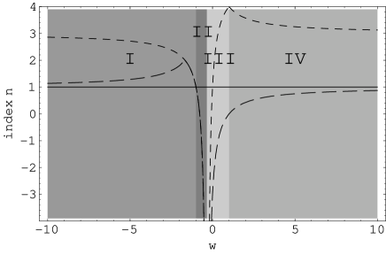
Figure 2: The short dashing line denotes $n_{\zeta}$, the long dashing line denotes $n_{\Phi}$. From left to right, the different shadows correspond to Region I II III and IV in table respectively.

Figure 3: The dashing line denotes $n_{t}$. From left to right, the different shadows correspond to Region I II III and IV in table respectively.

Therefore, in general, for various expanding and contracting phases the values of $n_{\Phi}$ and $n_{\zeta}$ are different. From (10) and (11),

$${{\cal H}^{\prime}\over{\cal H}^{2}}=-{1+3w\over 2}$$ (22)

can be obtained, thus

$$q={2\over 1+3w}$$ (23)

In term of relations between $n_{\Phi}$ or $n_{\zeta}$ and $q$, the Fig. 2 reflecting $n_{\Phi}$ or $n_{\zeta}$ varying with $w$ is plotted. $n_{t}$ is the spectrum index of the tensor fluctuations and plotted in Fig. 3. We see that only for $-{5\over 3}<w<-{1\over 3}$, i.e. $q<-{1\over 2}$, the spectrum index of $\zeta$ is the same as that of $\Phi$, and when $w\simeq-1$, nearly scale-invariant spectrum can be obtained, which corresponds to the case in inflationary cosmology, but for other value of $w$, the spectrum index of $\zeta$ is different from that of $\Phi$, the $\Phi$ spectrum is nearly scale-invariant for $w\ll-1$ and $\gg 1$, while the $\zeta$ spectrum is nearly scale-invariant for $w\simeq 0$. Which of the spectrum of $\Phi$ and $\zeta$ can be inherited in late-time observational cosmology dependent on the matching conditions through the “bounce” [8]. We shall briefly comment it in the following.

The curvature perturbations re-enter the horizon during radiation/matter-domination and create density fluctuations $\delta\rho$, which results in the formation of large-scale structure of universe. The density contrast $\delta={\delta\rho\over\rho}$ can deduced from Poisson equation

$$\delta_{k}={2\over 3}({k\over{\cal H}})^{2}\Phi_{k}$$ (26)

at horizon crossing ${\cal H}\simeq k$, $|\delta_{k}|^{2}\simeq|\Phi_{k}|^{2}$ is given, thus the Bardeen potential in late-time universe really determines the spectrum. The solution for $\Phi$ on super Hubble scale is approximately [25]

$$\Phi_{\pm}\simeq D_{\pm}+S_{\pm}{{\cal H}\over a^{2}}$$ (27)

From (16) and (17), we have

$$\zeta_{\pm}=\alpha D_{\pm}+\beta k^{2}S_{\pm}f(\eta)$$ (28)

where the subscript $+$ and $-$ denote the phases after and before the “bounce” respectively, the coefficient $D_{-}\sim k^{-{1\over 2}+q}$ and $D_{+}$ denote the amplitude of the constant mode, $S_{-}\sim k^{-{3\over 2}-q}$ and $S_{+}$ are that of the growing or decaying mode dependent on different phases, and $f(\eta)=\int({{\cal H}\over a\varphi^{\prime}})^{2}d\eta$, the coefficients $\alpha$ and $\beta$ are dependent only on the parameter $w$ of state equation. For late-time expanding phase driven by radiation/matter, $S_{+}$ is decaying mode, thus $D_{+}$ is dominated mode for our observational cosmology. If taking the constant energy hyper-surfaces, in which $\Phi$ and $\zeta$ are continuous across the bounce, i.e. the Deruelle-Mukhanov [27] (Hwang-Vishniac [28])matching conditions is satisfied, like that in the transition from inflationary phase to radiation dominated phase, $D_{+}\sim D_{-}$ can be obtained to leading order of $k$ [11], thus regardless which of $D_{-}$ and $S_{-}$ is dominated mode during pre-bounce phase, $D_{+}$ mode will only inherit the spectrum of $D_{-}$ mode. In this case we can obtain the same results from $\Phi$ and $\zeta$. But if, for example, we take $\Phi$ and $\Phi^{\prime}$ continuous, then $D_{+}\sim D_{-}+S_{-}$, which means that $D_{+}$ mode should take the spectrum of dominated mode which of $D_{-}$ and $S_{-}$. For ekpyrotic/cyclic and slowly expanding scenario, the growing $S_{-}$ mode is the dominated mode during pre-bounce phase, which will be inherited by $D_{+}$ mode. From (27) and (28), we see that for $S$ mode, the spectrum of $\Phi$ is different from that of $\zeta$ and the latter has a suppression from $k^{2}$, which may imply that $\zeta$ is not a proper quantity for the calculations of primordial perturbation spectrum in this case. More recently, as is pointed to in Ref.[9], see also Ref. [31, 30], the resulting spectral index in late radiation-dominated universe depends on how $\Phi$ and $\zeta$ passing through the “bounce”, which is determined by the details of “bouncing” physics.

In summary, we describe the evolution of various pre-bounce phases with constant $w$ and also construct the corresponding action of the single scalar field. We separate four different regions which correspond different expanding and contracting phases in term of parameter $w$ of state equation, and show that the inflation and other alternative scenarios recently proposed can be placed in different positions of these regions, and for all possible $w$, only when $w\simeq-1$ or $\ll-1$ or $\gg 1$ may the nearly scale-invariant scalar spectrum be obtained, which corresponds the inflation, ekpyrotic/cyclic and slowly expanding scenario respectively. The degeneration of nearly scale-invariant scalar fluctuations spectrum may be remove by the tensor fluctuations spectrum, see Fig. 3, which, for $w\simeq-1$, is nearly scale-invariant and for $w\ll-1$ or $\gg 1$, is strong blue. Since different scenarios make different predictions for the spectrum of scalar and tensor perturbations, it is possible that the observations of the cosmic microwave background can distinguish among different scenarios. For other value of $w$, the nearly scale-invariant scalar spectrum can not be generated by the fluctuations of background field, thus other feasible mechanisms may be required [33, 34, 35]. Furthermore, the matching between various phases [36, 37] may give a reasonable explain for a possible loss of power recently observated by WMAP. Our work offers an interesting classification for the primordial perturbation spectrum from various phases before the “bounce”, which may have important implications for building an early universe scenario embedded in possible high energy theories.

Acknowledgments We thank Mingzhe Li, Xinmin Zhang for useful discussions. We also thank Robert Brandenberger for reminding on the matching conditions in Ref. [11]. When this manuscript was being submitted to the relevant journal, Boyle et.al.’s paper appeared [38], in which the scalar pertrubations ($\Phi$ and $\zeta$) and tensor perturbations as a function of $w$ were also obtained, furthermore, they pointed out the interesting relationship between two different models sharing the same scalar perturbations. We thank its authors for kind correspondence and Paul J. Steinhardt for comments on our manuscript. This work is supported in part by K.C.Wang Postdoc Foundation and also in part by the National Basic Research Program of China under Grant No. 2003CB716300.

References

- [1] A.H. Guth, Phys. Rev. D23 (1981) 347; A.D. Linde, Phys. Lett. B108 (1982) 389; A.A. Albrecht and P.J. Steinhardt, Phys. Rev. Lett. 48 (1982) 1220.
- [2] A.D. Linde, hep-th/0402051.
- [3] C. Bennett et al., astro-ph/0302207; G. Hinshaw et. al., astro-ph/0302217; A. Kogut et. al., astro-ph/0302213.
- [4] J. Khoury, B.A. Ovrut, P.J. Steinhardt and N. Turok, Phys. Rev. D64 (2001) 123522; J. Khoury, B.A. Ovrut, N. Seiberg, P.J. Steinhardt and N. Turok, Phys. Rev. D65 (2002) 086007; P.J. Steinhardt and N. Turok, Science 296, (2002) 1436; Phys. Rev. D65 126003 (2002).
- [5] S. Gratton, J. Khoury, P.J. Steinhardt and N. Turok, astro-ph/0301395;
- [6] J. Khoury, P.J. Steinhardt and N. Turok, astro-ph/0302012.
- [7] A.J. Tolley, N. Turok and P.J. Steinhardt, hep-th/0306109.
- [8] R. Durrer, hep-th/0112026; R. Durrer and F. Vernizzi, Phys. Rev. D66 (2002) 083503.
- [9] C. Cartier, R. Durrer and E.J. Copeland, hep-th/0301198.
- [10] R. Kallosh, L. Kofman and A. Linde, Phys. Rev. D64 123523 (2001); R. Kallosh, L. Kofman, A. Linde and A. Tseytlin, Phys. Rev. D64, 123524 (2001).
- [11] R. Brandenberger and F. Finelli, JHEP 0111, 056 (2001).
- [12] J. Hwang, astro-ph/0109045; D.H. Lyth, Phys. Lett. B526,173 (2002); S. Tsujikawa, Phys. Lett. B526, 179 (2002); J. Martin, P. Peter, N. Pinto-Neto and D.J. Schwarz, Phys. Rev. D65, 123513 (2002).
- [13] S. Tsujikawa, R. Brandenberger and F. Finelli, Phys. Rev. D66, 083513 (2002).
- [14] A. Tolley and N. Turok, Phys. Rev. D66 (2002) 106005, hep-th/0204091.
- [15] M. Gasperini and G. Veneziano, Astropart. Phys. 1 (1993) 317, hep-th/9211021.
- [16] G. Veneziano, hep-th/0002094; J.E. Lidsey, D. Wands and E.J. Copeland, Phys. Rept. 337 (2000) 343, hep-th/9909061.
- [17] D. Wands, Phys. Rev. D60 023507 (1999); F. Finelli and R. Brandenberger, hep-th/0112249.
- [18] J.K. Erickson, D.H. Wesley, P.J. Steinhardt, N. Turok, hep-th/0312009.
- [19] Y.S. Piao and E Zhou, Phys. Rev. D68, 083515 (2003).
- [20] L.F. Abbott and M.F. Wise, Nucl. Phys. B244, 541 (1984).
- [21] L. Kofman, A.D. Linde and A.A. Starobinski, Phys. Rev. Lett. 73 3195 (1994); Phys. Rev. D56 3258 (1997).
- [22] G.N. Felder, L. Kofman and A.D. Linde, Phys. Rev. D59 123523 (1999); Phys. Rev. D60 103505 (1999).
- [23] Y.S. Piao and Y.Z. Zhang, astro-ph/0401231.
- [24] V.F. Mukhanov, JETP lett. 41, 493 (1985); Sov. Phys. JETP. 68, 1297 (1988).
- [25] V.F. Mukhanov, H.A. Feldman and R.H. Brandenberger, Phys. Rept. 215, 203 (1992).
- [26] A.A. Starobinsky, JETP Lett 30, 682 (1979).
- [27] N. Deruelle and V.F. Mukhanov, Phys. Rev. D52 5(1995).
- [28] J. Hwang and E.T. Vishniac, Astrophs. J. 382 (1991).
- [29] C. Gordon and N. Turok, Phys. Rev. D67 (2003) 123508.
- [30] J. Martin and P. Peter, hep-th/0307077.
- [31] P. Peter and N. Pinto-Neto, hep-th/0203013; P. Peter, N. Pinto-Neto and D.A. Gonzalez, hep-th/0306005.
- [32] Finelli, hep-th/0307068.
- [33] D.H. Lyth, and D. Wands, hep-ph/0110002; S. Mollerach, Phys.Rev. D42 (1990) 313; K. Enqvist, and M. S. Sloth, hep-ph/0109214; T. Moroi and T. Takahashi, hep-ph/0110096.
- [34] V. Bozza, M. Gasperini, M. Giovannini and G. Veneziano, hep-ph/0206131; hep-ph/0212112.
- [35] G. Dvali, A. Gruzinov and M. Zaldarriaga, Phys. Rev. D69 (2004) 023505; L. Kofman, astro-ph/0303614.
- [36] Y.S. Piao, B. Feng and X. Zhang, Phys. Rev. D in press, hep-th/0310206.
- [37] Y.S. Piao, S. Tsujikawa and X. Zhang, hep-th/0312139.
- [38] L.A. Boyle, P.J. Steinhardt and N. Turok, hep-th/0403026.