Principal Component Analysis of AGN Spectra

Abstract

We discuss spectral principal component analysis (SPCA) and show examples of its application in analyzing AGN spectra in both small and large samples. It can be used to identify peculiar spectra and classify AGN spectra. Its application to correlation studies of AGN spectral properties and spectral measurements for large samples is promising.

University of Texas at Austin, Austin, TX 78712

University of Texas at Austin, Austin, TX 78712

1. Introduction

To study AGN spectra, one has to deal with many emission features as well as continuum. Simple statistics often cannot handle the large number of measured parameters efficiently, therefore, a multivariate analysis is needed. Principal component analysis (PCA) is one such powerful tool (see also Boroson 2004).

Suppose we have $n$ AGNs in a sample, each has $p$ measured parameters $X_{1},X_{2},\cdots,X_{p}$. We can write

$$\begin{array}[]{ccccc}&X_{1}&X_{2}&\cdots&X_{p}\\ QSO1&x_{11}&x_{12}&\cdots&x_{1p}\\ QSO2&x_{21}&x_{22}&\cdots&x_{2p}\\ \vdots&\vdots&\vdots&&\vdots\\ QSOn&x_{n1}&x_{n2}&\cdots&x_{np}\\ \end{array}.$$

$X_{1},X_{2},\cdots,X_{p}$ are unit vectors and $x_{ij}$ are data.

PCA defines a set of new orthogonal variables, principal components $W_{j}$ ($j=1,\cdots,p$), which are linear combinations of the original variables
$W_{j}=e_{j1}X_{1}+e_{j2}X_{2}+\cdots+e_{jp}X_{p},$ (1)
An easy way to understand PCA is to consider it from the geometrical point of view (Francis & Wills 1999). PCA aims to define orthogonal principal axes in a multi-dimensional space, as shown in Fig. 1, where a correlation exists between measured parameters $X_{1}$ and $X_{2}$, and two principal components (PCs) are defined. PC1 (or $W_{1}$) accounts for most variance (the correlation), PC2 (or $W_{2}$) is small and can be ignored.

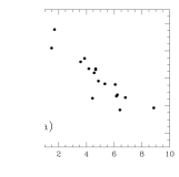
Figure 1.: Geometrical point of view of PCA. (a) Measured values. (b) Mean subtracted values. Two principal axes PC1 and PC2 are defined.

PCA can be applied to AGN spectra directly (Francis et al. 1992; Shang et al. 2003). In this spectral principal component analysis (SPCA), each spectrum is divided into small wavelength bins, and the flux in each bin (e.g., $F_{\lambda_{i}}$) is an input variable. Eq. (1) can be written as
$W_{j}=e_{j1}F_{\lambda_{1}}+e_{j2}F_{\lambda_{2}}+\cdots+e_{jp}F_{\lambda_{p}},$ (2)
The result principal components can then be also represented as spectra, $SPC_{j}=[e_{j1}\ e_{j2}\ \cdots\ e_{jp}]$, namely, the spectral principal components (SPCs). An original spectrum can be reconstructed by adding the weighted principal component spectra to the mean spectrum,
$Spectrum_{i}=Mean+w_{i1}{SPC_{1}}+w_{i2}{SPC_{2}}+\cdots+w_{ip}{SPC_{p}},$
where $w_{ij}$ are calculated from Eq. 2 for each object $i$, and are referred as the weights (or scores) of $SPC_{j}$. In other words, all original spectra are made from the principal component spectra. This implies that a limited number of SPCs can be used to measure spectra in large samples (see also Yip et al. 2004).

If there are strong linear relationships among the original variables (or wavelength bins), each of these relationships will be represented by a principal component. Fewer principal components may be required to describe the total variation of a sample, thus providing a simpler description of the dataset (Francis et al. 1992). Any principal component accounting for a significant fraction of the total sample variance might be related to one or more underlying fundamental physical parameters, giving some physical insight into the cause of the variations (Boroson & Green 1992, Boroson 2002). However, PCA is only a statistical tool and it is still up to the investigators to judge whether the resulting PCs have any physical meanings.

PCA is a linear analysis. If there are strong non-linear relationships involved, PCA is not able to identify them directly and there will be crosstalk among the resulting principal components. When a non-linear part of a relationship is not strong, PCA is still able to follow the “linear” trend of the relationship. In SPCA, good redshifts are needed because line shifts can cause strong non-linear effects. Line width change also introduces non-linear relationships among binned fluxes, so caution is needed in interpreting SPCA results.

2. SPCA on a Small Sample of Quasars

Shang et al. (2003) show the power of SPCA in analyzing a small sample of QSOs. SPCA decomposes the QSO spectra into three independent, significant principal components (Fig. 2). SPC1 represents the Baldwin effect, but only line-cores are involved. By using SPC1 instead of integrated line EW, the scatter in the luminosity relationship is reduced. SPC2 shows changes of UV-optical continuum slope, due to intrinsic QSO continuum slope variation and/or reddening. SPC3 extends Boroson & Green’s Eigenvector 1 relationship (Boroson & Green 1992), to include many UV line properties and line-width changes.

Figure 2.: Mean spectrum and the three significant spectral principal components from SPCA for the small sample (Shang et al. 2003). The numbers in parenthesis are the fractions of the sample variance accounted for by each principal component. Spectral features in opposite directions in the principal components are anti-correlated, and vice versa. The “W” shape of Ly$\alpha$, Mg ii, H$\beta$, and H$\alpha$ in SPC3 indicates that the width increases with stronger [O iii]. The very broad “small blue bump” is anticorrelated with the optical Fe ii features.

3. SPCA on Large Samples

One of the advantages of SPCA is that correlations can be investigated without parameterizing the line profiles or defining the continua. Therefore, it is especially useful for analyzing large samples.

Also unlike the “composite spectrum analysis”, SPCA analysis keeps the information for individual objects, e.g., the weights of the principal component spectra for each object, which can be used to correlate with other non-spectral properties, such as black hole mass etc. SPCA has also been used for classifying AGN spectra (e.g., Francis et al. 1992, Boroson 2002).

To demonstrate its use for large samples, we applied SPCA to the SDSS DR1 QSO spectra in the region of Ly$\alpha$-C iv-C iii]. We choose only 771 objects with high redshift-confidence ($\verb"z_conf">0.95$) (Stoughton et al. 2002). For a sample with uniform spectral properties, the distribution of the weights of SPCs should be random and centered at the origin. However, there are outliers in the distribution of the weights of SPC1 and SPC2 (Fig. 3, left), indicating that these spectra are peculiar (Fig. 3, right).

Figure 3.: Left: Distribution of the weights of SPC1 and SPC2 with all 771 spectra. The outliers have peculiar spectra. Right: Examples of peculiar spectra selected with SPCA.

We are interested in the spectral properties of the majority of the sample, so after excluding the peculiar spectra, SPCA is applied to the remaining 639 spectra. Fig. 4 (left) shows the first three principal components which can be used to classify the spectra and investigate the correlations among the spectra properties. SPC1 shows that the line-cores are correlated with each other, similar to the SPC1 in Sec. 2, but the expected Baldwin effect has large scatter (Fig. 4, right). SPC2 shows line-width change: strong-SPC2 objects have narrow Ly$\alpha$. SPC3 shows absorptions (or line shifts) in Ly$\alpha$ and C iv; strong-SPC3 objects have Ly$\alpha$ and C iv absorptions.

Figure 4.: Left: SPCA results for 639 spectra. Right: Continuum luminosity vs. SPC1 (line-core). The scatter in the anticorrelation ($P<10^{-4}$) is large. The luminosity is calculated with the measured continuum flux at 1682Å assuming H₀=50, q₀=0.5.

References

Boroson, T.A. & Green, R. 1992, ApJS, 80, 109

Boroson, T.A. 2002, ApJ, 565, 78

Boroson, T.A. 2004, this volume.

Francis, P.J., Hewett, P.C., Foltz, C.B. & Chaffee, F.H. 1992, ApJ, 398, 476

Francis, P. & Wills, B.J. 1999, in ASP Conf. Series 162, Quasars and Cosmology, ed. G.J. Ferland & J.A. Baldwin (San Francisco: ASP), 363

Shang, Z., Wills, B., Robinson, E., Wills, D., Laor, A. et al. 2003, ApJ, 568, 52

Stoughton, C. et al. 2002, ApJ, 123, 485

Yip, Ching-Wa, Connolly, A., Vanden Berk, D. et al. 2004, this volume.