Dark Matter Relic Abundance and Scalar-Tensor Dark Energy

Abstract

Scalar-tensor theories of gravity provide a consistent framework to accommodate an ultra-light quintessence scalar field. While the equivalence principle is respected by construction, deviations from General Relativity and standard cosmology may show up at nucleosynthesis, CMB, and solar system tests of gravity. After imposing all the bounds coming from these observations, we consider the expansion rate of the universe at WIMP decoupling, showing that it can lead to an enhancement of the dark matter relic density up to few orders of magnitude with respect to the standard case. This effect can have an impact on supersymmetric candidates for dark matter.

I Introduction

According to our current understanding rev-cosmo , Dark Matter (DM) and Dark Energy (DE) represent the two major components of the present Universe. Surprisingly, it is found that the DM and DE energy densities, $\rho_{DM}$ and $\rho_{DE}$, are today roughly the same (differing only by a factor of two), while their ratio has been varying by several orders of magnitude in the past history of the Universe.

It seems quite natural, then, to explore the possibility of a DM–DE interaction which could account for this coincidence. This approach, however, is not free from problems if the DE component is interpreted in terms of a dynamical quintessence quint-review scalar field. Indeed, such a scalar is constrained to be extremely light in order to fit the data, giving rise to unwanted long-range forces which may represent a severe threat to the equivalence principle. In addition, couplings of the quintessence scalar with the gauge field strengths are potential sources of dangerous time variations of the fundamental constants.

A possible way of coping with a very light scalar while avoiding these shortcomings, is to choose to work in the framework of a scalar-tensor gravity (ST) theory bd , where by construction matter has a purely metric coupling with gravity. It has been shown max that in this case, the scalar field can benefit from an attraction mechanism which, during the matter dominated era, makes ST overlapping with standard General Relativity (GR). At the same time, ST may possess a second “attraction mechanism” max which will ensure the correct evolution of $\rho_{DE}$ along a so-called ‘tracking’ tracker solution.

While ST can very closely reproduce standard GR at the present time, it may however lead to major differences in the past evolution of the Universe, differences which may result in observable consequences for us today. For example, it has been shown joyce ; damour-pichon ; santiago ; carroll2 that ST theories may have a profund impact on nucleosynthesis. At the same time, a curious fact has recently come to attention: a non–conventional dynamics of the quintessence scalar in the past history of the universe may remain ‘hidden’ to the available cosmological observations, but manifest itself through the DM relic abundance salatirosati ; ullio ; comelli . It is then worth studying if ST may provide a viable quintessence candidate and at the same time have an impact on the DM relic abundance. We have considered this possibility and computed explicitly the differences from the standard case.

When considering ST theories, the departures from standard cosmology are mainly due to the different expansion rate ($\tilde{H}$) which they determine. Such deviation from the usual expansion rate of GR bears potentially relevant consequences in all those phenomena which are closely dependent on the timing in which they occur. The aim of the present work is to study the possible modifications of the expansion rate of the Universe in ST at the time of Cold Dark Matter (CDM) freeze-out, focussing on Weekly Interacting Massive Particles (WIMPs) as the most natural candidates for CDM. As it is well known, their present relic density depends on the precise moment they decouple and, in turn, on the precise moment the WIMP annihilation rate equals the expansion rate of the Universe. We expect then that a variation of $\tilde{H}$ in the past may lead to measurable consequences on the WIMP relic abundance.

In order to assess the allowed departure of $\tilde{H}$ from its standard value at WIMPs freeze-out, we have to take into account the bounds imposed on ST by phenomena at later epochs Riaz . We already mentioned the crucial test of nucleosynthesis: passing the BBN exam will imply rather severe restrictions on the coupling of the scalar field of ST to matter and also on its initial conditions at temperatures much higher than the WIMP freeze-out. Coming to later epochs, we have to consider the photon decoupling and the consequent restrictions imposed by CMB data CMB . Interestingly enough, we will show that the BBN “filter” on ST is so efficient that it drastically limits any visible effect on the CMB spectrum (in particular, shifts in the peaks positions are forced to be smaller than the experimental error). More restrictive than the CMB probe turn out to be the GR tests, in particular after the tight bound on the post-newtonian parameter $\gamma$, recently provided by the Cassini spacecraft cassini . This constraint becomes quite relevant when combined with that on the scalar equation of state of $w_{\phi}$ coming from SNe Ia data SNe . We will find that significant deviations from standard cosmology are possible only if the DE equation of state differs appreciably from $-1$ today. In other words, if DE is a cosmological constant, it is unlikely that future cosmological observations will be able to discriminate between ST and GR.

The question we intend to explicitly tackle is the following: taking all the abovementioned restrictions (BBN, CMB, GR tests) into account, how much can the Hubble parameter $\tilde{H}$ at the time of WIMP freeze-out differ from its canonical value if ST replaces GR? In other words, how much is the WIMP relic density allowed to vary, if we consider ST instead of GR?

We find that in ST theories the expansion rate of the Universe at few GeVs can profoudly differ from the usual value obtained in GR (with variations up to five orders of magnitude) and, yet, allow the correct light elements production at BBN. This situation is perfectly analogous to the ‘kination’ effect studied in salatirosati , where a modification of $\tilde{H}$ at WIMP freeze-out was induced by a short period of dominance of the scalar kinetic energy, although with some deal of fine-tuning. In the case considered here, the effect of ST on $\tilde{H}$ depends on the strength of the scalar-matter coupling, however no particular fine-tuning is needed to pass the severe nucleosynthesis test even when large modifications of $\tilde{H}$ at freeze-out occur. This means that the attraction of ST towards GR proceeds very rapidly during the cooling of the Universe from the few GeVs of WIMPs freeze-out down to the MeV range of nucleosynthesis. The overlap of ST with GR can subsequently be very efficient leading to ST scenarios which can hardly be disentangled from ordinary GR in present tests at the post-newtonian level. The fact that ST strongly affects the number of CDM particles may turn out to be the major signature of these theories.

¿From the point of view of particle physics model building, these large variations in the WIMPs number density today is of utmost relevance. Particles which were not considered suitable to play a significant role in CDM scenarios can be rescued because of their enhanced number density. On the other hand, particles (or regions of the parameter space for certain WIMPs candidates), which in usual GR scenarios constitute promising CDM candidates, would be excluded because their boosted number would overclose the Universe. These considerations become of particular interest if we focus on the case where the WIMPs correspond to the lightest supersymmetric particle. A complete analysis of the cosmologically excluded and cosmologically interesting regions of the SUSY parameter spaces in different SUSY contexts, when ST is considered, is presently in progress inprogress .

II Scalar-tensor theories of gravity

ST theories represent a natural framework in which massless scalars may appear in the gravitational sector of the theory without being phenomenologically dangerous. In these theories a metric coupling of matter with the scalar field is assumed, thus ensuring the equivalence principle and the constancy of all non-gravitational coupling constants dam . Moreover, as discussed in dam3a ; dam3b , a large class of these models exhibit an attractor mechanism towards GR, that is, the expansion of the Universe during the matter dominated era tends to drive the scalar fields toward a state where the theory becomes indistinguishable from GR.

ST theories of gravity are defined by the action dam ; dam3a ; dam3b

$$S=S_{g}+S_{m}\,,$$ (1)

where

$$S_{g}=\frac{1}{16\pi}\int d^{4}x\sqrt{-\tilde{g}}\left[\Phi^{2}\tilde{R}\;+\right.$$

$$\quad\quad+\left.4\,\omega(\Phi)\tilde{g}^{\mu\nu}\partial_{\mu}\Phi\partial_{\nu}\Phi-4\tilde{V}(\Phi)\right]\,.$$ (2)

The matter fields $\Psi_{m}$ are coupled only to the metric tensor $\tilde{g}_{\mu\nu}$ and not to $\Phi$, i.e. $S_{m}=S_{m}[\Psi_{m},\tilde{g}_{\mu\nu}]$. $\tilde{R}$ is the Ricci scalar constructed from the physical metric $\tilde{g}_{\mu\nu}$. Each ST model is identified by the two functions $\omega(\Phi)$ and $\tilde{V}(\Phi)$. For instance, the well-known Jordan-Fierz-Brans-Dicke (JFBD) theory bd corresponds to $\omega(\Phi)=\omega$ (constant) and $\tilde{V}(\Phi)=0$.

The matter energy-momentum tensor is conserved, masses and non-gravitational couplings are time independent, and in a locally inertial frame non gravitational physics laws take their usual form. Thus, the ‘Jordan’ frame variables $\tilde{g}_{\mu\nu}$ and $\Phi$ are also denoted as the ‘physical’ ones in the literature. On the other hand, the equations of motion are rather cumbersome in this frame, as they mix spin-2 and spin-0 excitations. A more convenient formulation of the theory is obtained by defining two new gravitational field variables, $g_{\mu\nu}$ and the dimensionless field $\varphi$, by means of the conformal transformation

$$\tilde{g}_{\mu\nu} \equiv \displaystyle A^{2}(\varphi)g_{\mu\nu}$$

$$\Phi^{2} \equiv \displaystyle 8\pi M_{\ast}^{2}A^{-2}(\varphi)$$

$$V(\varphi) \equiv \displaystyle\frac{A^{4}(\varphi)}{4\pi}\tilde{V}(\Phi)$$

$$\alpha(\varphi) \equiv \displaystyle\,\frac{d\log A(\varphi)}{d\varphi}\,.$$ (3)

Imposing the condition

$$\alpha^{2}(\varphi)=\frac{1}{4\omega(\Phi)+6}\,,$$ (4)

the gravitational action in the ‘Einstein frame’ reads

$$S_{g}=\frac{M_{\ast}^{2}}{2}\int d^{4}x\sqrt{-{g}}\left[{R}+{g}^{\mu\nu}\partial_{\mu}\varphi\partial_{\nu}\varphi-\frac{2}{M_{\ast}^{2}}V(\varphi)\right],$$ (5)

and matter couples to $\varphi$ only through a purely metric coupling,

$$S_{m}=S_{m}[\Psi_{m},A^{2}(\varphi){g}_{\mu\nu}]\,\,\,.$$ (6)

In this frame masses and non-gravitational coupling constants are field-dependent, and the energy-momentum tensor of matter fields is not conserved separately, but only when summed with the scalar field one. On the other hand, the Einstein frame Planck mass $M_{\ast}$ is time-independent and the field equations have the simple form

$$R_{\mu\nu}-\mbox{\small$\frac{1}{2}$}g_{\mu\nu}R=\displaystyle\frac{T^{\varphi}_{\mu\nu}}{M_{\ast}^{2}}+\frac{T_{\mu\nu}}{M_{\ast}^{2}}$$

$$\displaystyle\partial^{2}\varphi+\frac{1}{M_{\ast}^{2}}\frac{\partial V}{\partial\varphi}=-\frac{1}{M_{\ast}^{2}}\frac{\alpha(\varphi)}{\sqrt{2}}T\,,$$ (7)

where

$$T^{\varphi}_{\mu\nu}=M_{\ast}^{2}\partial_{\mu}\varphi\partial_{\nu}\varphi-g_{\mu\nu}\left[M_{\ast}^{2}\frac{g^{\rho\sigma}}{2}\partial_{\rho}\varphi\partial_{\sigma}\varphi-V(\varphi)\right]\,,$$

and $T_{\mu\nu}=2(-g)^{-1/2}\,\delta S_{m}/\delta g^{\mu\nu}$ is the matter energy-momentum tensor in the Einstein frame. The relevant point about the scalar field equation in (7) is that its source is given by the trace of the matter energy-momentum tensor, $T\equiv g^{\mu\nu}T_{\mu\nu}$, which implies the (weak) equivalence principle. Moreover, when $\alpha(\varphi)=0$ the scalar field is decoupled from ordinary matter and the ST theory is indistinguishable from ordinary GR.

We next consider an homogeneous cosmological space-time

$$ds^{2}=dt^{2}-a^{2}(t)\ dl^{2}\ ,$$

where the matter energy-momentum tensor admits the perfect-fluid representation

$$T^{\mu\nu}=(\rho+p)\ u^{\mu}u^{\nu}\ -p\ g^{\mu\nu}\ \ ,$$

with $g_{\mu\nu}\ u^{\mu}u^{\nu}=1$.

The Friedmann-Robertson-Walker (FRW) equations then take the form

$$\frac{\ddot{a}}{a} = -\frac{1}{6M_{\ast}^{2}}\left[\rho+3\ p+2M_{\ast}^{2}\dot{\varphi}^{2}-2V(\varphi)\right]$$ (8)

$$\left(\frac{\dot{a}}{a}\right)^{2}+\frac{k}{a^{2}} = \frac{1}{3M_{\ast}^{2}}\left[\rho+\frac{M_{\ast}^{2}}{2}\dot{\varphi}^{2}+V(\varphi)\right]$$ (9)

$$\ddot{\varphi}+3\frac{\dot{a}}{a}\dot{\varphi} = -\frac{1}{M_{\ast}^{2}}\left[\frac{\alpha(\varphi)}{\sqrt{2}}(\rho-3p)+\frac{\partial V}{\partial\varphi}\right]\ ,$$ (10)

with the Bianchi identity

$${}d(\rho a^{3})+p\ da^{3}=(\rho-3\ p)\ a^{3}d\log A(\varphi).$$ (11)

The physical proper time, scale factor, energy, and pressure, are related to their Einstein frame counterparts by the relations

$$d\tilde{\tau}=A(\varphi)d\tau\,,\;\;\tilde{a}=A(\varphi)a\,,\;\;\tilde{\rho}=A(\varphi)^{-4}\rho\,,\;\;\tilde{p}=A(\varphi)^{-4}p.$$

Defining new dimensionless variables

$$N\equiv\log\frac{a}{a_{0}},\qquad\qquad\lambda\equiv\frac{V(\varphi)}{\rho},\qquad\qquad w\equiv\frac{p}{\rho},$$

and setting $k=0$ (flat space) the field equation of motion takes the more convenient form

$$\frac{2}{3}\;\frac{1+\lambda}{1-{\varphi^{\prime}}^{2}/6}\ \varphi^{\prime\prime}+[(1-w)+2\lambda]\varphi^{\prime}=$$

$$\quad\quad\quad\quad\quad-\sqrt{2}\;\alpha(\varphi)\;(1-3w)-2\;\lambda\;\frac{d\log V(\varphi)}{d\varphi},$$ (12)

where primes denote derivation with respect to $N$. This will be our master equation.

The effect of the early presence of a scalar field on the physical processes will come through the Jordan-frame Hubble parameter $\tilde{H}\equiv d\log\tilde{a}/d\tilde{\tau}$:

$$\tilde{H}=H\,\frac{(1+\alpha(\varphi)\,\varphi^{\prime})}{A(\varphi)}\,,$$ (13)

where $H\equiv d\log a/d\tau$ is the Einstein frame Hubble parameter. In the flat–space case ($k=0$), Eq (13) finally gives:

$$\tilde{H}^{2}=\frac{A^{2}(\varphi)}{3M_{*}^{2}}\,\frac{\left(1+\alpha(\varphi)\,\varphi^{\prime}\right)^{2}}{1-(\varphi^{\prime})^{2}/6}\,\left[\tilde{\rho}+\tilde{V}\right]\,\,\,\,.$$ (14)

III Evolution of the field

III.1 Radiation domination

During radiation domination the scalar field energy density is suppressed, $\lambda\ll 1$, and the first term in the RHS of Eq. (12) is proportional to

$$1-3w=\frac{\rho_{\rm tot}-3p_{\rm tot}}{\rho_{\rm tot}}=\frac{\tilde{\rho}_{\rm tot}-3\tilde{p}_{\rm tot}}{\tilde{\rho}_{\rm tot}}$$

$$\quad\quad\quad\quad=\frac{1}{\tilde{\rho}_{\rm tot}}\left[\sum_{A}(\tilde{\rho}_{A}-3\tilde{p}_{A})+\tilde{\rho}_{m}\right]\,,$$ (15)

where the sum runs over all particles in thermal equilibrium, while $\tilde{\rho}_{m}$ is the contribution from the decoupled and pressureless matter abundance.

During radiation domination, $\tilde{\rho}_{\rm tot}\simeq\pi^{2}T^{4}/30$, where $T$ is the Jordan-frame temperature, and the contribution from a single particle in equilibrium gives

$$\frac{\tilde{\rho}_{A}-3\tilde{p}_{A}}{\tilde{\rho}_{\rm tot}}\simeq\frac{15}{\pi^{4}}\frac{g_{A}}{g_{\star}}y_{A}^{2}F[y_{A}]\,,$$ (16)

with $y_{A}\equiv m_{A}/T$, $g_{A}$ the number of degrees of freedom of A, $g_{\star}$ the number of relativistic degrees of freedom and

$$F[y_{A}]\equiv\int_{0}^{\infty}dx\frac{x^{2}}{\varepsilon_{A}[\exp(\varepsilon_{A})\pm 1]}\,,$$ (17)

where $\varepsilon_{A}\equiv(y_{A}^{2}+x^{2})^{1/2}$ and the minus (plus) sign in the denominator of the integrand holds for bosons (fermions). In Fig. 1 we plot $y^{2}F[y]$. We see that it is different from zero only around $y=1$, that is, for $T\simeq m_{A}$. For higher temperatures it is quadratically suppressed in $y$, approaching the relativistic regime in which $1-3\tilde{w}_{A}=0$. For lower temperatures it is Boltzmann- suppressed. Then, as emphasized in dam3a ; dam3b , the field $\varphi$ evolves even during radiation domination, receiving a ‘kick’ each time a particle in equilibrium becomes non-relativistic. The second term in Eq. (15) is suppressed as $T_{\rm eq}/T$, so it becomes relevant only as equivalence is approached.

In the following, we will consider the evolution of the field from the freeze out of the DM particles down to today, so we will have to take into account all particles of masses between the freeze-out and matter-radiation equivalence.

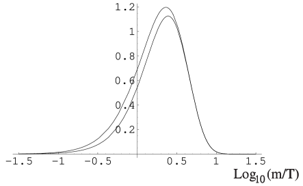
Figure 1: The function $y^{2}F[y]$, with $y\equiv m/T$ defined by Eq. (17). The upper (lower) curve corresponds to bosons (fermions).

III.2 Matter domination

During matter domination $1-3w\simeq 1$ and, as long as the field energy density is subdominant ($\lambda\ll 1$), the RHS of the equation of motion (12) is given by $-\sqrt{2}\alpha(\varphi)$ and the field evolution depends on the form of the coupling function $\alpha(\varphi)$. As already mentioned, the JBD theory is given by a constant $\alpha$, and the value $\alpha=0$ corresponds to GR. A very attractive class of models is that in which the function $\alpha(\varphi)$ has a zero with a positive slope, since this point, corresponding to GR, is an attractive fixed point for the field equation of motion dam3a ; dam3b .

It was emphasized in Ref. max (see also sabino2 ) that the fixed point starts to be effective around matter-radiation equivalence, and that it governs the field evolution until recent epochs, when the quintessence potential becomes dominant. If the latter has a run-away behavior, the same should be true for $\alpha(\varphi)$, so that the late-time behavior converges to GR.

III.3 Late-time beahavior

The evolution of the field during the last redshifts depends on the nature of DE. We will consider two possibilities: a cosmological constant and a inverse-power law scalar potential for $\varphi$, which can be collectively represented by the potential

$$V(\varphi)=\Lambda^{4}\varphi^{-\delta}\qquad\qquad(\delta\geq 0),$$ (18)

$\delta=0$ corresponding to the cosmological constant.

In general, a cosmological constant in the Einstein frame does not correspond to a cosmological constant in the Jordan frame, as one can read from Eq. (3). However, present tests of GR (see next section) imply that at late times $A(\varphi)\simeq 1$, so that the two frames are almost coincident and the expansion histories during the last few redshifts are practically indistinguishable.

For the purpose of this paper, that is the analysis of the impact of DE on ST cosmology, the situation in which the quintessence field is different from $\varphi$ and decoupled from it would be basically the same as that with a cosmological constant, since in both cases the second term in the RHS of Eq. (12) vanishes.

The main feature of the potential in (18) for $\delta>0$ is the existence of ‘tracker’ solutions, which are attractors in field space tracker . In the $\alpha\to 0$ limit, the late-time behavior is completely determined by the two parameters $\bar{\lambda}\equiv\Lambda^{4}/\rho_{M}^{0}$ and $\delta$. A non-vanishing $\alpha$ would modify the behavior of the field today, hopefully keeping the desirable property of insensitivity to the initial conditions.

In this paper, we will consider the following choice for $A(\varphi)$,

$$A(\varphi)=1+Be^{-\beta\varphi}\,,$$ (19)

corresponding to

$$\alpha(\varphi)=-\frac{\beta Be^{-\beta\varphi}}{1+Be^{-\beta\varphi}}\,,$$ (20)

which has a run-away behavior with positive slope, as required by the discussion at the end of the previous subsection. The choice for the parameters $B$ and $\beta$ will be discussed in the following section.

In Fig. 2 we show the evolution of the background and field energy density. We see that field energy densities corresponding to different initial conditions converge to the same solution, driven by $\alpha(\varphi)$. Notice also that the $\alpha$-attractor becomes effective even before matter-radiation equivalence, due to the non-relativistic decoupling effect explained above.

In Fig. (3) we show the region of parameter plane $\bar{\lambda}$-$\delta$ giving $w_{\varphi}<-0.7$, where

$$w_{\varphi}=\frac{M_{\ast}^{2}/2\;\dot{\varphi}^{2}-V(\varphi)}{M_{\ast}^{2}/2\;\dot{\varphi}^{2}+V(\varphi)}\,,$$ (21)

and $0.65<\Omega_{\varphi}<0.75$. We see that in the ST case, ($B\neq 0$) the region giving more negative values of the equation of state is somehow enlarged with respect to pure GR quintessence. However, in the observationally allowed region for $\Omega_{\varphi}$ the influence of the $B$ parameter is negligible.

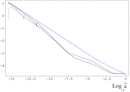
Figure 2: Evolution of the energy density of the background (upper solid line) and of three typical solutions for the scalar field. We see that different initial conditions converge to the same solution.

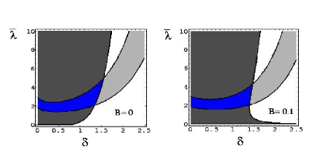
Figure 3: The regions in the $\bar{\lambda}$-$\delta$ parameter plane giving $w_{\varphi}<-0.7$ (dark grey) and $0.65<\Omega_{\varphi}<0.75$ (light grey). The left plot is the pure GR case ($B=0$) while the right one is for ST with $B=0.1$, $\beta=8$.

IV Phenomenological bounds

IV.1 Nucleosynthesis

Assuming $\alpha\varphi^{\prime}\simeq 0$ in Eq. (14) – as we have checked numerically for the solutions relevant in this analysis – the Jordan frame expansion rate during nucleosynthesis may be approximated as

$$\tilde{H}^{2}\simeq A^{2}(\varphi)\frac{1}{3M_{\ast}^{2}}\tilde{\rho}\,.$$ (22)

The above expression should be compared to the GR one, in which the Planck mass at nucleosynthesis was the same as today. We obtain:

$$\left.\frac{\Delta\tilde{H}^{2}}{\tilde{H}^{2}}\right|_{\rm nuc}\equiv\left.\frac{\tilde{H}^{2}-\tilde{H}_{\rm GR}^{2}}{\tilde{H}_{\rm GR}^{2}}\right|_{\rm nuc}=\frac{A^{2}(\varphi_{nuc})-A^{2}(\varphi_{0})}{A^{2}(\varphi_{0})}\,.$$ (23)

The change in the expansion rate is completely analogous to that obtained by adding extra neutrinos to the standard GR case. Using the bound $\Delta N<1$ (which is more restrictive than those obtained for instance in nubound ), we get

$$\frac{A(\varphi_{nuc})}{A(\varphi_{0})}<1.08\,.$$ (24)

IV.2 General relativity tests

At the post-newtonian level, the deviations from GR may be parametrized in terms of an effective field-dependent newtonian constant

$$G=G(\varphi)\equiv G_{*}A(\varphi)^{2}(1+\alpha^{2}(\varphi))\,,$$

and two dimensionless parameters $\gamma_{PN}$ and $\beta_{PN}$ which, in the present theories turn out to be dam

$$\gamma_{PN}-1=-2\frac{\alpha^{2}}{1+\alpha^{2}}\,,\,\,\,\,\beta_{PN}-1=\frac{\kappa\alpha^{2}}{(1+\alpha^{2})^{2}}\,,$$ (25)

where $\kappa=\partial\alpha/\partial\varphi$.

A new constraint on the parameter $\gamma_{PN}$ has been obtained recently using radio links with the Cassini spacecraft cassini ,

$$\gamma_{PN}-1=(2.1\pm 2.3)\times 10^{-5}.$$ (26)

Present bounds on $\beta_{PN}-1$ are $O(10^{-4})$ and are less restrictive for our choice of $\alpha(\varphi)$, since $\kappa_{0}\alpha^{2}(\varphi_{0})\simeq-\beta\alpha^{3}(\varphi_{0})$.

The bound from the Cassini spacecraft turns out to be quite strong when used in connection with the one on the equation of state $w_{\varphi}$ from SNe Ia. In Fig. (4) we show the excluded region in the $\beta$-$w_{\varphi}$ plane implied by Eq. (26). We see that an equation of state $w_{\varphi}<-0.78$, as implied by Sne Ia data at $95\%$ c.l. SNe , requires either a large value for $\beta$, or a very small $B$. Since the last case corresponds to an expansion history of the universe practically indistinguishable from GR, any non-standard behavior induced by the ST theories in the past should be likely accompanied by an equation of state different from $-1$ today. If DE is a pure cosmological constant, then the bound from Cassini implies $B<O(10^{-3})$ (making $A(\varphi)$ practically indistinguishable from one at least since BBN on), or unnaturally large values of $\beta$.

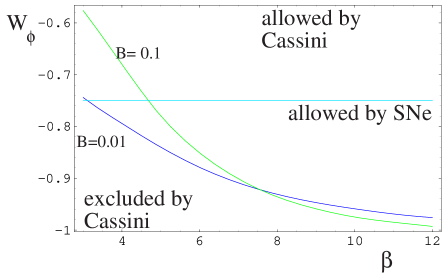
Figure 4: The impact of the Cassini GR test. The regions below the curves are excluded at $1\sigma$ level. The SNIa bound on the DE equation of state is also shown.

IV.3 CMB power spectrum

The impact of a cosmological constant or quintessence on the CMB power spectrum has been extensively analyzed in refs. DEonCMB . In the context of ST theories, the problem has been studied in Refs. Riaz ; Sabino . The main change with respect to a theory for DE based on GR is due to a difference in the expansion rate, which affects the angular scale of the anisotropies. The angle under which the first peak is seen goes as

$$\theta_{\rm peak}\sim\pi/l_{\rm peak}\sim v_{s}\,t_{\rm dec}\,z_{\rm dec}/d(z_{\rm dec})\,,$$ (27)

where $l_{\rm peak}$ is the corresponding multipole, $v_{s}$ is the sound speed, $t_{\rm dec}$ and $z_{\rm dec}$ are the time and redshift of decoupling, and $d(z_{\rm dec})$ the distance to the last scattering surface. The latter is given by

$$d(z_{\rm dec})=\int_{1/(z_{\rm dec}+1)}^{1}\,\frac{d\tilde{a}}{\tilde{a}\tilde{H}}\,,$$ (28)

and is thus dominated by the behavior of $\tilde{H}$ close to the upper limit of integration, where $\tilde{a}\tilde{H}$ is smaller. For this reason, ST theories passing the GR tests ($A\to 1$ today, that is, $\tilde{H}\to\tilde{H}_{\rm GR}$) imply a small deviation of the distance to the last scattering surface with respect to GR.

On the other hand, the decoupling time might be significantly more perturbed. It is given by an expression analogous to Eq. (28) with the upper (lower) limit of integration replaced by $1/(z_{\rm dec}+1)$ ($0$). As a result, since the universe expanded faster than in GR at early times, we expect $t_{\rm dec}$ to be smaller, and the peak to move towards higher multiples. We find

$$\frac{\Delta l_{\rm peak}}{l_{\rm peak}}\simeq\frac{4}{3}\frac{A(\tilde{a}_{\rm dec})-1}{A(\tilde{a}_{\rm dec})}\,,$$ (29)

which is consistent with the numerical findings of ref. Riaz .

Due to the well known degeneracy of the CMB spectrum with respect to cosmological parameters, present measurements of the peak locations CMB do not translate straightforwardly into a bound on $A(\tilde{a}_{\rm dec})$. For instance, it is found that a shift in the peak multipole can be obtained also by varying the energy densities according to huth-turner

$$\frac{\Delta l_{\rm peak}}{l_{\rm peak}}\simeq -1.25\frac{\Delta\Omega}{\Omega}$$ (30)

$$-0.23\frac{\Delta\Omega_{M}h^{2}}{\Omega_{M}h^{2}}+0.09\frac{\Delta\Omega_{b}h^{2}}{\Omega_{b}h^{2}}+0.089\frac{\Delta\Omega_{M}}{\Omega_{M}}\,,$$

so that, in general, a full reanalysis of the CMB including the new parameter $A(\tilde{a}_{\rm dec})$ would be required. However, in the present case we find that, once the BBN bound on $A$ has been imposed, the resulting values for $A(\tilde{a}_{\rm dec})$ are so close to unity as to give shifts in the peak multiples smaller than the experimental error. Thus, the CMB spectrum does not provide significant bounds to the present scenario.

V Impact on WIMP relic abundance

Having in mind all the bounds discussed in the previous Section, we can now go on to compute the cosmological evolution of the scalar field and its impact on the DM relic abundance.

As a first step, we want to estimate if ST can have a sizeable effect on the Jordan-frame Hubble parameter $\tilde{H}$ at the time of WIMP decoupling, without violating any of the avaliable cosmological observations. We will consider the function $A(\varphi)$ of Eq. (19), imposing on the parameters $B$ and $\beta$ the phenomenological constraints already discussed. We will then compute the ratio $\tilde{H}/\tilde{H}_{\rm GR}$ at the decoupling time of a typical WIMP of mass $m=200$ GeV. In this way we will be able to get an estimate of the effect before going into further detail.

The tightest bound is that coming from Eq. (24). It has an impact on both $B$ in Eq. (19) and on the initial conditions of $\varphi$ at temperatures higher than the WIMP freeze-out. Indeed, since on the tracker solution the scalar field is $\varphi_{0}^{\rm tr}=O(1)$ today, it should have been $\ll 1$ at nucleosynthesis, otherwise it would not have reached the attractor in time tracker . This implies $B\leq O(0.1)$.

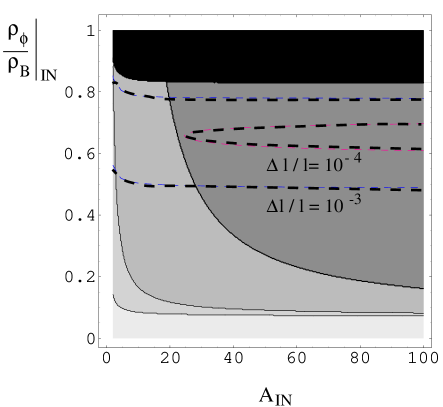
Figure 5: The contours show the expansion rate enhancement $\tilde{H}/\tilde{H}_{\rm GR}$ at $T=10$ GeV obtained in the ST model, as a function of the initial values of the factor $A(\varphi)$ and of the ratio of the scalar to background energy density $\rho_{\varphi}/\rho_{B}$. We considered for the initial conditions a temperature of $T=500$ GeV. The black area represents initial conditions which are excluded by nuclesynthesis. The grey contours represent enhancements of $1\div 10^{2}$, $10^{2}\div 10^{3}$, $10^{3}\div 10^{4}$, $10^{4}\div 10^{5}$ from the lightest to the darkest. The dashed lines show the shifts of the CMB doppler peaks obtained in the ST model.

As already discussed, the equation for the dynamics of the scalar field $\varphi$ is obtained by substituting the expression of Eq. (15) in the RHS of Eq. (12) and choosing a coupling function $\alpha(\varphi)$ as defined in Eq. (20). In the sum of Eq. (15) only the terms corresponding to particles with $m<T_{c}$ have been considered, i.e. particles lighter than the critical temperature of the phase transition through which they acquire a mass (see Ref. dam3b ). In particular we have taken into account the top quark, the $Z^{0}$, the $W^{\pm}$, the bottom quark, the tau quark, the charmed quark, the pions, the muon, the electron and a WIMP particle of mass $m=200$ GeV. Numerical integration of the equation for $\varphi$ has been carried out between approximately 500 GeV and today. We have then computed, through Eq.(14), the modified expansion rate in the ST theory at a temperature $T=10$ GeV corresponding to a typical time of WIMP decoupling and compared it to the expansion rate of the standard case at the same temperature.

In Fig. 5 we plot the ratio $\tilde{H}/\tilde{H}_{\rm GR}$ at $T=10$ GeV as a function of the initial value of $A(\varphi)$ and initial ratio of the scalar to background energy density $\rho_{\varphi}/\rho_{B}$. We have restricted the possible initial conditions to those regions of parameters values respecting the BBN bound of Eq. (24). We see that we have been able to produce an enhancement of the expansion rate up to $O(10^{5})$ at the time of WIMP decoupling. It is then worth studying in more detail what happens to the WIMP relic abundance.

Let us now consider the calculation of the relic abundance of a DM WIMP with mass $m$ and annihilation cross-section $\langle\sigma_{\rm ann}v\rangle$. As already mentioned, laboratory clocks and rods measure the “physical” metric $\tilde{g}_{\mu\nu}$ and so the standard laws of non-gravitational physics take their usual form in units of the interval $d\tilde{s}^{2}$. As outlined in Ref.damour-pichon , the effect of the modified ST gravity will enter the computation of particle physics processes (like the WIMP relic abundance) through the “physical” expansion rate $\tilde{H}$ defined in Eq. (13). We have therefore to implement the standard Boltzmann equation with the modified physical Hubble parameter $\tilde{H}$:

$$\frac{dY}{dx}=-\frac{1}{x}\frac{s}{\tilde{H}}\langle\sigma_{\rm ann}v\rangle(Y^{2}-Y_{\rm eq}^{2})$$ (31)

where $x=m/T$, $s=(2\pi^{2}/45)~{}h_{\star}(T)~{}T^{3}$ is the entropy density and $Y=n/s$ is the WIMP density per comoving volume.

Figure 6: A typical behaviour of the function $A(\varphi)$ defined in Eq. (19), calculated for parameters $B=0.1$ and $\beta=8$.

We have considered values of $\tilde{H}$ wich respect all the bounds discussed in Section IV. Specifically, we have considered the function $A(\varphi)$ as given in Eq. (19) with parameters $B=0.1$ and $\beta=8$. The function $A(\varphi)$ for this choice of parameters is plotted in Fig. 6, which shows that $A(\varphi)$ is very large at large temperatures, and then, at a temperature $T_{\varphi}$, sharply drops to values close to 1 before nucleosynthesis sets in. A parametrization of the behaviour of $A(\varphi)$ for $T>T_{\varphi}$, that will be useful in the following discussion, is:

$$A(\varphi) \simeq 2.19\cdot 10^{14}\left(\frac{T_{0}}{T}\right)^{0.82}$$ (32)

$$\simeq 9.65\cdot 10^{3}\left(\frac{\rm GeV}{m}\right)^{0.82}\,x^{0.82}$$

where $T_{0}$ is the current temperature of the Universe.

We have numerically checked that, in the regime we are considering, a good approximation to the physical Hubble parameter is given by:

$$\tilde{H}=A(\varphi)\tilde{H}_{\rm GR}$$ (33)

The solution of the Boltzmann equation is therefore formally the same as in the standard case, with the noticeable difference that now the Hubble parameter gets an additional temperature dependence, given by the function $A(\varphi)$. This can be translated in a change in the effective number of degrees of freedom at temperature $T$:

$$g_{\star}(x)\longrightarrow A^{2}(x)g_{\star}(x)$$ (34)

An approximated solution of Eq.(31) can be cast in a form analogous to the standard case:

$$\frac{1}{Y_{0}}=\frac{1}{Y_{f}}+\sqrt{\frac{\pi}{45G}}~{}m\int_{x_{f}}^{\infty}dx\,\frac{A^{-1}(x)\,G(x)\langle\sigma_{\rm ann}v\rangle}{x^{2}}$$ (35)

where $G(x)=h_{\star}(x)/g^{1/2}_{\star}(x)$ and $Y_{0}$ and $Y_{f}$ are the WIMP abundances per comovin volume today and at freeze–out, respectively.

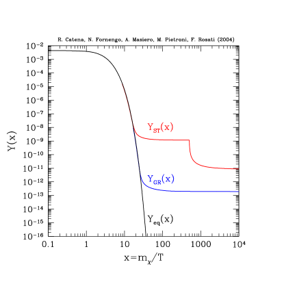
Figure 7: Numerical solution of the Boltzmann equation Eq. (31) in a ST cosmology for a toy–model of a DM WIMP of mass $m=50$ GeV and constant annihilation cross-section $\langle\sigma_{\rm ann}v\rangle=1\times 10^{-7}$ GeV^-2. The temperature evolution of the WIMP abundance $Y(x)$ clearly shows that freeze–out is anticipated, since the expansion rate of the Universe is largely enhanced by the presence of the scalar field $\varphi$. At a value $x=m/T_{\varphi}$ a re–annihilation phase occurs and $Y(x)$ drops to the present day value.

The freeze–out temperature is obtained by the following implicit equation:

$$x_{f}=\ln\left[0.038\,M_{P}\,g\,m\,\frac{\langle\sigma_{\rm ann}v\rangle_{f}\,x_{f}^{-1/2}}{A(x_{f})g^{1/2}_{\star}(x_{f})}\right]$$ (36)

where $g$ is the internal number of degrees of freedom of our WIMP. Clearly, when $A(x)\rightarrow 1$ we recover the standard case. The relic abundance is then simply given by:

$$\Omega h^{2}=\frac{m\,s_{0}\,Y_{0}}{\rho_{\rm crit}}$$ (37)

where $s_{0}$ is the present entropy density and $\rho_{\rm crit}$ denotes the critical density.

A numerical solution of the Boltzmann equation Eq. (31) in a ST cosmology with the function $A(x)$ given in Fig. 6 is shown in Fig. 7 for a toy–model of a DM WIMP of mass $m=50$ GeV and constant annihilation cross-section $\langle\sigma_{\rm ann}v\rangle=1\times 10^{-7}$ GeV^-2. The temperature evolution of the WIMP abundance $Y(x)$ clearly shows that freeze–out is anticipated, since the expansion rate of the Universe is largely enhanced by the presence of the scalar field $\varphi$. This effect is expected. However, we note that a peculiar effect emerges: when the ST theory approached GR (a fact which is parametrized by $A(\varphi)\rightarrow 1$ at a temperature $T_{\varphi}$, which in our model is 0.1 GeV), $\tilde{H}$ rapidly drops below the interaction rate $\Gamma$ establishing a short period during which the already frozen WIMPs are still abundant enough to start a sizeable re–annihilation. This post-freeze–out “re–annihilation phase” has the effect of reducing the WIMP abundance, which nevertheless remains much larger than in the standard case. For the specific case shown in Fig. 7 the WIMP relic abundance is $\Omega h^{2}=0.0027$ for GR, while for a ST cosmology becomes $\Omega h^{2}=0.12$, with an increase of a factor of 44.

The phenomenon of re–annihilation can be conveniently discussed in terms of the relation between the expansion rate of the Universe $\tilde{H}$ and the WIMP interaction rate $\Gamma=Y\,s\,\langle\sigma_{\rm ann}v\rangle$. A numerical calculation of these two quantities is plotted in Fig. 8 as a function of the temperature. The departure from equilibrium occurs earlier than in the GR case, because $\tilde{H}\gg\tilde{H}_{\rm GR}$. When decoupling is completed, the particles evolve with an approximately constant $Y=Y_{f}$ and $\Gamma\sim T^{3}$, while the Hubble rate evolves as $\tilde{H}\sim A(x)\,\tilde{\rho}^{1/2}\,\sim T^{1.2}$, i.e. slower than in the standard case (we have used here the approximate $A(x)$ behavious of Eq.(32)).

At the transition temperature $T_{\varphi}$ the Hubble rate drops to its standard value $H_{\rm GR}$ and becomes smaller than the interaction rate: in this case the decoupled WIMPs start to annihilate again, for a short period. After this re–annihilation phase, the particles continue to evolve with an approximately constant abundace $Y<Y_{f}$ and $\Gamma$ recovers the behaviour $T^{3}$, while $\tilde{H}_{\rm GR}\sim\tilde{\rho}^{1/2}\sim T^{2}$ as usual.

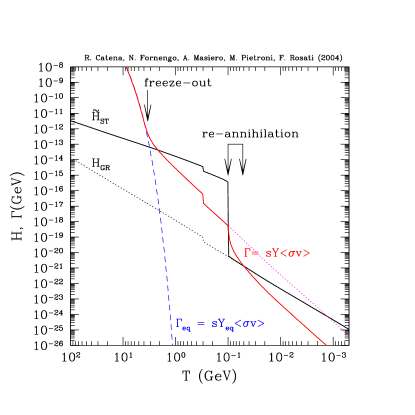
Figure 8: The Expansion rate of the Universe $\tilde{H}$ and the WIMP interaction rate $\Gamma=Y\,s\,\langle\sigma_{\rm ann}v\rangle$ are plotted as a function of the temperature. The re-annihilation effect discussed in the text is outlined. The small drop in the rates at $T=300$ MeV is due to the quark–hadron phase transition.

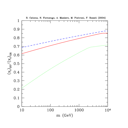
Figure 9: The ratio between the freeze–out values of $x_{f}=m/T_{f}$ in ST cosmology and in GR as a function of the WIMP mass. The dashed, solid and dotted lines refer to $\langle\sigma_{\rm ann}v\rangle=10^{-4}$ GeV^-2, $10^{-7}$ GeV^-2 and $10^{-14}$ GeV^-2, respectively.

We notice that a re–annihilation phase does not occur in the case of kination, i.e. in the case the energy density of the Universe is dominated by the kinetic term of a scalar field salatirosati . In this case the evolution of the expansion rate is $\tilde{H}_{\rm kin}\sim T^{3}$ during kination, and than evolves smootly into the standard behaviour $\tilde{H}_{\rm GR}\sim T^{2}$. During kination both $\tilde{H}$ and $\Gamma$ have the same $T$–dependence and closely follow each other, until kination ends and the standard behaviour is recovered. Re–annihilation is possibile if the phase during which the expansion rate has the transition toward its standard GR behaviour is faster than the post-freeze–out evolution of the interaction rate, i.e. faster than $T^{3}$.

The change in the freeze–out temperature is shown in Fig. 9 where we show the ratio between the freeze–out values of $x_{f}=m/T_{f}$ in ST cosmology and in GR. The freeze–out temperature is anticipated about a factor of 2, with a dependence also on the annihilation cross section, as is clear from Eq. (36): for very low values of $\langle\sigma_{\rm ann}v\rangle$ the freeze-out temperature may be anticipated up to a factor of 5. For these low cross sections the relic abundance is anyway largely overabundant: we can therefore quantify the reduction in $x_{f}$ in a factor which ranges between 10% and 40% for WIMPs which can provide abundances in the cosmologically acceptable range.

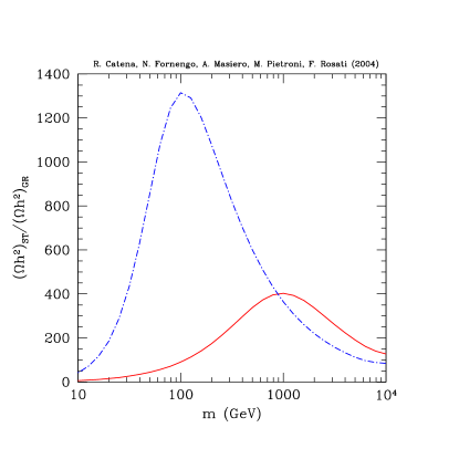
Figure 10: Increase in the WIMP relic abundance in ST cosmology with respect to the GR case. The solid curve refers to an annihilation cross section constant in temperature, i.e. $\langle\sigma_{\rm ann}v\rangle=a=10^{-7}$ GeV^-2, while the dashed line stands for an annihilation cross section which evolves with temperature as $\langle\sigma_{\rm ann}v\rangle=b/x=10^{-7}$ GeV${}^{-2}/x$.

The amount of increase in the relic abundance which is present in ST cosmology is shown in Fig. 10. The solid curve refers to an annihilation cross section constant in temperature, i.e. $\langle\sigma_{\rm ann}v\rangle=a$, while the dashed line stands for an annihilation cross section which evolves with temperature as: $\langle\sigma_{\rm ann}v\rangle=b/x$ (these two cases correspond to the two limiting situations of the usual non–relativistic expansion of the thermally averaged annihilation cross section: $\langle\sigma_{\rm ann}v\rangle=a+b/x$). In the case of $s$–wave annihilation the increase in relic abundance ranges from a factor of 10 up to a factor of 400. For a pure $b/x$ dependence, the enhancement can be as large as 3 orders of magnitude.

The behaviours shown in Fig. 10, which have been obtained by a numerical integration of the Boltzmann equation Eq. (31), can be understood by employing the approximate analytical solution (35). In the case of $\langle\sigma_{\rm ann}v\rangle=a$, Eq. (35) gives:

$$\frac{1}{Y_{0}}={\cal G}\,m\,G(x^{\rm GR}_{f})\frac{a}{x^{\rm GR}_{f}}$$ (38)

in the standard GR case, and

$$\frac{1}{Y_{0}} = {\cal G}\,m\left[\frac{G(x_{f}^{ST})}{\bar{A}}\frac{a}{1.82}\left(\frac{1}{(x_{f}^{ST})^{1.82}}-\frac{1}{(x_{\varphi})^{1.82}}\right)\right]$$ (39)

$$+ {\cal G}\,m\left[G(x_{\varphi})\frac{a}{x_{\varphi}}\right]$$

in our ST model where the $A(x)$ function is given in Eq. (32) for $T>T_{\varphi}$ and $A(x)=1$ otherwise (${\bar{A}}=9.65\cdot 10^{3}({\rm GeV}/m)^{0.82}$). For the sake of simplicity, in both solutions we have dropped the term $1/Y_{f}$ which adds a small correction, not relevant for the present approximate discussion. In both equations ${\cal G}=\sqrt{\pi/(45\,G)}$. The ratio $R$ of the relic abundances is:

$$R\equiv\frac{(\Omega h^{2})_{\rm ST}}{(\Omega h^{2})_{\rm GR}}\simeq\frac{1.82\,\bar{A}\,x_{\varphi}\,x_{f}^{0.82}}{x_{\varphi}+1.82\,\bar{A}\,r_{G}\,x_{f}^{1.82}}$$ (40)

where we have approximated $x^{\rm GR}_{f}\simeq x^{ST}_{f}$ and we have defined $r_{G}=G(x_{\varphi})/G(x_{f})$. By making explicit the mass dependencies we obtain:

$$R\simeq\frac{A_{R}\,m_{\rm GeV}}{B_{R}+m_{\rm Gev}^{1.82}}$$ (41)

where the mass is expresses in GeV, $A_{R}\simeq 1.76\cdot 10^{4}\,x_{f}^{0.82}\simeq 2.05\cdot 10^{5}$, $B_{R}=1.76\cdot 10^{4}\,T_{\varphi}\,r_{G}\,x_{f}^{1.82}\simeq 2.05\cdot 10^{5}$, and the numerical values have been obtained for $x_{f}\simeq 20$ and $r_{G}\simeq 0.5$ (since in our case $T_{\varphi}$ is smaller than the quark–hadron phase transition which we have set at $T_{\rm QCD}=300$ MeV). The analytic approximation of Eq. (41) helps to explain the behaviour shown by the solid curve in Fig. 10, which has been obtained by numerical calculations which employ the exact form of the function $A(\varphi)$. From Eq. (41) we can in fact derive that, for low masses, the ratio $R$ has the behaviour:

$$R\simeq\frac{m}{r_{G}\,T_{\varphi}}\,\frac{1}{x_{f}}=\frac{1}{r_{G}}\,\frac{T_{f}}{T_{\varphi}}$$ (42)

which shows that in this mass regime $R$ grows almost linearly with the WIMP mass $m$, and it is larger for lower values of $T_{\varphi}$. If we accept $T_{\varphi}$ as low as the BBN scale, we can obtain a further increase in the relic abundance of a factor 100 on the top of the one showed in Fig. 11 for low values of $m$. When the WIMP mass is very large, the ratio $R$ behaves as:

$$R\simeq\frac{1.76\cdot 10^{4}\,x_{f}^{0.82}}{m_{\rm GeV}^{0.82}}$$ (43)

with a slight drop with the mass. The position of the maximum and the maximal value of $R$ are given by:

$$m^{\rm max}_{\rm GeV}\simeq(2.15\cdot 10^{4}\,r_{G}\,T_{\varphi})^{0.56}\,\,x_{f}$$ (44)

and:

$$R_{\rm max}\simeq\frac{108}{(r_{G}T_{\varphi})^{0.45}}$$ (45)

These expressions show that the maximal effect is also obtained for the lowest values of $T_{\varphi}$; in this case the position of $R_{\rm max}$ is shifted toward lower masses. For $T_{\varphi}$ at the BBN scale, the maximal increase in the WIMP relic abundance is of the order of 3000, instead of about 400 obtained for $T_{\varphi}=0.1$ GeV and shown in Fig. 11.

An interesting property shown by Eq. (41) is that $R$ does not depend explicitely on the annihilation cross section $\langle\sigma_{\rm ann}v\rangle=a$, which drops out in the ratio. An implicit dependence on the cross section is present through $x_{f}$, as can be seen in Eq. (36). This dependence however is only logarithmic and does not spoil the general behaviour of $R$ shown in Fig. 10. This is shown in Fig. 11: the largest difference occurs for very low annihilation cross sections, for which the deviation of $x_{f}$ is larger. However, for cross sections of interest, i.e. cross section which provide relic abundances below the cosmologically acceptable upper bound, the values of $R$ are stable to a relatively good extent.

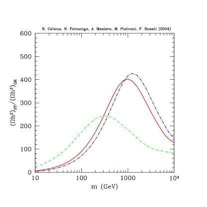
Figure 11: Increase in the WIMP relic abundance with an annihilation cross section $\langle\sigma_{\rm ann}v\rangle=a$, for different values of $a$. The dot–dashed, solid and dashed lines correspond to $a=10^{-4}$ GeV^-2, $10^{-7}$ GeV^-2 and $10^{-14}$ GeV^-2, respectively.

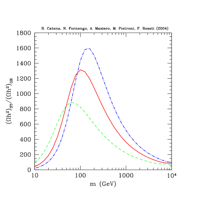
Figure 12: Increase in the WIMP relic abundance with an annihilation cross section $\langle\sigma_{\rm ann}v\rangle=b/x$, for different values of $b$. The dot–dashed, solid and dashed lines correspond to $b=10^{-4}$ GeV^-2 $10^{-7}$ GeV^-2 and $10^{-10}$ GeV^-2, respectively.

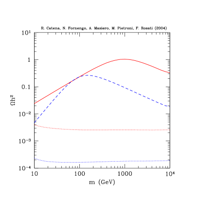
Figure 13: The relic abundance in a ST theory as a function of the WIMP mass in the case of $\langle\sigma_{\rm ann}v\rangle\equiv a=1\cdot 10^{-7}$ GeV (solid line) and $\langle\sigma_{\rm ann}v\rangle\equiv b/x=1\cdot 10^{-4}~{}{\rm GeV}/x$ (dashed line). The upper (lower) dotted lines corresponds to the GR case for $\langle\sigma_{\rm ann}v\rangle\equiv a=1\cdot 10^{-7}$ GeV and $\langle\sigma_{\rm ann}v\rangle\equiv b/x=1\cdot 10^{-4}~{}{\rm GeV}/x$, respectively.

A similar analysis holds in the case of $\langle\sigma_{\rm ann}v\rangle=b/x$. However, in this case the dependence of $R$ with $x_{f}$ is somehow stronger (as obtained from the integration in Eq. (35)), and the effect of changing $\langle\sigma_{\rm ann}v\rangle$ is slightely larger. This effect can be seen in Fig. 12, where $R$ is shown for different values of the parameter $b$. Notice that larger cross sections, which in the standard case provide lower values for the relic abundance, are the ones which get more enhanced in ST cosmology.

Finally, as an example we show in Fig. 13 the relic abundance as a function of the WIMP mass in the case of $\langle\sigma_{\rm ann}v\rangle\equiv a=1\cdot 10^{-7}$ GeV and $\langle\sigma_{\rm ann}v\rangle\equiv b/x=1\cdot 10^{-4}~{}{\rm GeV}/x$. We see that, in this case, the relic abundance can be at the level required to explain the CDM content of the Universe ($\Omega_{\rm CDM}h^{2}=0.095\div 0.13$ wmap ) for a ST theory, while it is underabundant in the standard case. The models shown in Fig. 13 represent a case in which we can explain at the same time both the DM and DE contents of the Universe, and the interplay of the two component is crucial in determinig the right abundances of both DM and DE.

An analysis of specific particle candidates of DM, in particular in supersymmetric models, will be examined elsewhere inprogress .

VI Conclusions

The idea of exploiting primordial (ultralight) scalars in order to shed some light on a dynamical interpretation of DE is by now a widespread research topic in the literature. In this paper we follow the promising proposal of considering the quintessence scalar as embedded in a scalar–tensor theory of gravity. This approach is at variance with the usual interpretation of quintessence as a new light scalar whose interactions with matter are subject to the tight phenomenological constraints on the equivalence principle violation and time-variation of the fundamental coupling constants. Identifying the quintessence field with the scalar component of a ST theory, instead, does not pose any threat on the equivalence principle, since by construction matter has a purely metric coupling with gravity.

We focus on quintessence ST models which possess a double “attraction mechanism”, one to GR and the other ensuring $\rho_{DE}$ to follow a tracking solution. These two simultaneous mechanisms act as a “protection” for the theory to prevent its fall into immediate troubles (for instance, large departures from GR predictions). Nevertheless, we still obtain important phnomenological signatures which might disentangle this theory from GR or other alternative proposals. The tests of our ST scenario divide into two classes: deviations from GR and departures from standard cosmology, in particular concerning the expansion rate of the Universe.

The latter effect has a big impact on the most distant epoch of the Universe for which we have “direct” information, i.e. nucleosynthesis. However, we pointed out that we can further extend the implications of a non-standard $\tilde{H}$ in the early Universe to times prior to nucleosynthesis. Sticking to the standard WIMP picture of DM, one of the most relevant events before BBN is the WIMP decoupling which is expected to have occurred at a temperature of a few GeVs. Our work shows that, despite the severe “filters” on ST quintessence models which are provided by BBN, solar system tests of gravity and, to a lesser degree, by CMB, it is still possible to find remarkable enhancements on the expansion rate of the Universe at WIMP freeze-out, yielding to relic WIMP abundances which can vary up to a few orders of magnitude with respect to the standard case.

In this paper we pointed out some general features of the new “WIMP story” around its decoupling temperature in the presence of ST quintessence. In particular, we noticed that some unexpected effect can take place, such as a short phase of WIMP “re-annihilation” when ST approaches GR. Needless to say, such potentially (very) large deviations entail new prospects on the WIMP characterization both for the choice of the CDM candidates and for their direct and indirect detection probes. A thorough reconsideration of the “traditional” WIMP identified with the lightest neutralino in SUSY extensions of the SM as well as the identification of other potentially viable CDM candidates in the ST context is presently under way inprogress .

VII Aknowledgments

We acknowledge Research Grants funded by the Italian Ministero dell’Istruzione, dell’Università e della Ricerca (MIUR) and by the Istituto Nazionale di Fisica Nucleare (INFN) within the Astroparticle Physics Project. FR is partially supported by the University of Padova fund for young researchers, research project n. $CPDG037114$.

References

- (1) W. L. Freedman and M. S. Turner, Rev. Mod. Phys. 75 (2003) 1433.
- (2) For recent reviews, see for example: S. M. Carroll, Living Rev. Rel. 4 (2001) 1; P. J. E. Peebles and B. Ratra, Rev. Mod. Phys. 75 (2003) 559; T. Padmanabhan, Phys. Rept. 380 (2003) 235.
- (3) S. M. Carroll, Phys. Rev. Lett. 81 (1998) 3067.
- (4) A. Masiero, M. Pietroni and F. Rosati, Phys. Rev. D 61 (2000) 023504.
- (5) T. Damour, F. Piazza and G. Veneziano, Phys. Rev. D 66 (2002) 046007; T. Damour, F. Piazza and G. Veneziano, Phys. Rev. Lett. 89 (2002) 081601
- (6) T. Damour and K. Nordtvedt, Phys. Rev. D48, 3436 (1993).
- (7) T. Damour and A.M. Polyakov, Nucl. Phys. B423, 532 (1994).
- (8) P. Jordan, Schwerkaft und Weltall (Vieweg, Braunschweig, 1955); M. Fierz, Helv. Phys. Acta 29, 128 (1956); C. Brans and R.H. Dicke, Phys. Rev. 124, 925 (1961).
- (9) N. Bartolo and M. Pietroni, Phys. Rev. D 61 (2000) 023518
- (10) A. R. Liddle and R. J. Scherrer, Phys. Rev. D 59 (1999) 023509; I. Zlatev, L. M. Wang and P. J. Steinhardt, Phys. Rev. Lett. 82 (1999) 896; P. J. Steinhardt, L. M. Wang and I. Zlatev, Phys. Rev. D 59 (1999) 123504; B. Ratra and P. J. E. Peebles, Phys. Rev. D 37 (1988) 3406; P. J. E. Peebles and B. Ratra, Astrophys. J. 325 (1988) L17.
- (11) M. Joyce and T. Prokopec, JHEP 0010 (2000) 030; M. Joyce, Phys. Rev. D 55 (1997) 1875.
- (12) T. Damour and B. Pichon, Phys. Rev. D 59 (1999) 123502.
- (13) D.I. Santiago, D. Kalligas and R.V. Wagoner, Phys. Rev. D58 (1998) 124005.
- (14) S. M. Carroll and M. Kaplinghat, Phys. Rev. D 65 (2002) 063507.
- (15) P. Salati, Phys. Lett. B 571, 121 (2003); F. Rosati, Phys. Lett. B 570, 5 (2003).
- (16) S. Profumo and P. Ullio, JCAP 0311 (2003) 006
- (17) D. Comelli, M. Pietroni and A. Riotto, Phys. Lett. B 571 (2003) 115; M. Kamionkowski and M. S. Turner, Phys. Rev. D 42, 3310 (1990); J. D. Barrow, Nucl. Phys. B 208 (1982) 501.
- (18) A. Riazuelo and J. P. Uzan, Phys. Rev. D 66, 023525 (2002).
- (19) P. de Bernardis et al., Astrophys. J. 564, 559 (2002); R. Stompor et al., Astrophys. J. 561, L7 (2001); C. L. Bennett et al., Astrophys. J. Suppl. 148, 1 (2003).
- (20) B. Bertotti, L. Iess and P. Tortora, Nature 425, 374 (2003)
- (21) A. G. Riess et al. [Supernova Search Team Collaboration], Astron. J. 116, 1009 (1998); S. Perlmutter et al. [Supernova Cosmology Project Collaboration], Astrophys. J. 517, 565 (1999); J. L. Tonry et al., Astrophys. J. 594, 1 (2003); B. J. Barris et al., Astrophys. J. 602, 571 (2004); A. G. Riess et al., Astrophys. J. 607, 665 (2004).
- (22) R. Catena, N. Fornengo, A. Masiero, M. Pietroni and F. Rosati, in progress
- (23) T. Damour, gr-qc/9606079, lectures given at Les Houches 1992, SUSY95 and Corfú 1995.; G. Esposito-Farese and D. Polarski, Phys. Rev. D 63, 063504 (2001); B. Boisseau, G. Esposito-Farese, D. Polarski and A. A. Starobinsky, Phys. Rev. Lett. 85, 2236 (2000).
- (24) S. Matarrese, C. Baccigalupi and F. Perrotta, astro-ph/0403480.
- (25) E. Lisi, S. Sarkar and F. L. Villante, Phys. Rev. D 59 (1999) 123520; K. A. Olive and D. Thomas, Astropart. Phys. 11, 403 (1999).
- (26) D. Huterer and M. S. Turner, Phys. Rev. D 64, 123527 (2001); S. Hannestad and E. Mortsell, Phys. Rev. D 66, 063508 (2002); A. Balbi, C. Baccigalupi, F. Perrotta, S. Matarrese and N. Vittorio, Astrophys. J. 588, L5 (2003).
- (27) X. l. Chen and M. Kamionkowski, Phys. Rev. D 60, 104036 (1999); F. Perrotta, C. Baccigalupi and S. Matarrese, Phys. Rev. D 61, 023507 (2000); R. Nagata, T. Chiba and N. Sugiyama, Phys. Rev. D 69, 083512 (2004); R. Nagata, T. Chiba and N. Sugiyama, Phys. Rev. D 66, 103510 (2002).
- (28) D. Huterer and M. S. Turner, Phys. Rev. D 64 (2001) 123527
- (29) D.N. Spergel et al., Astrophys. J. Suppl. 148, 175 (2003).