The Mass Discrepancy-Acceleration Relation:
Disk Mass and the Dark Matter Distribution

Abstract

The mass discrepancy in disk galaxies is shown to be well correlated with acceleration, increasing systematically with decreasing acceleration below a critical scale $a_{0}\approx 3700\;{\mathrm{km}^{2}\,\mathrm{s}^{-2}\,\mathrm{kpc}^{-1}}=1.2\times 10^{-10}\;\mathrm{m}\,\mathrm{s}^{-2}$. For each galaxy, there is an optimal choice of stellar mass-to-light ratio which minimizes the scatter in this mass discrepancy-acceleration relation. The same mass-to-light ratios also minimize the scatter in the baryonic Tully-Fisher relation and are in excellent agreement with the expectations of stellar population synthesis. Once the disk mass is determined in this fashion, the dark matter distribution is specified. The circular velocity attributable to the dark matter can be expressed as a simple equation which depends only on the observed distribution of baryonic mass. It is a challenge to understand how this very fine-tuned coupling between mass and light comes about.

1 Introduction

The masses of stellar disks and the distribution of mass in dark matter halos pose a coupled problem. Rotation curves provide good measures of the mass enclosed by disks. But it has been difficult to disentangle how much of this mass is in the stellar disk, and how much is in the dark matter halo. Consequently, both the mass of the stellar disk and the distribution of the dark matter, $\rho(r)$, have been unclear.

There have long been suggestions of a close connection between mass and light in spiral galaxies. Perhaps the most obvious is the Tully-Fisher relation (Tully & Fisher 1977). Beyond this global scaling relation, there are indications of a local coupling between mass and light (e.g., Rubin et al. 1985; Bahcall & Casertano 1985; Persic & Salucci 1991). One manifestation of this is in the efficacy of maximum disk (e.g., van Albada & Sancisi 1986) in describing the inner parts of rotation curves. If one scales up the stellar contribution to the rotation curves of high surface brightness (HSB) spirals to the maximum allowed by the data, one often finds a good match in the details (the “bumps and wiggles”) between the shape of the rotation curve and that predicted by the observed stellar mass (e.g., Kalnajs 1983; Sellwood 1999; Palunas & Williams 2000). This only works out to some radius where dark matter must be invoked, but does suggest that the preponderance of the mass at small radii is stellar. Beyond that, it is often possible to scale up the gas component to explain the remainder of the rotation curve (Hoekstra, van Albada, & Sancisi 2001). Moreover, while some dark matter may be needed to stabilize disks, detailed analyses of disk stability frequently require rather heavy disks in order to drive the observed bars and spiral features (e.g., Athanassoula, Bosma, & Papaioannou 1987; Debattista & Sellwood 1998, 2000; Weiner, Sellwood, & Williams 2001; Fuchs 2003a; Bissantz, Englmaier, & Gerhard 2003; Kranz, Slyz, & Rix 2003).

While these lines of evidence favor nearly maximal disks in HSB spirals, there are contradictory indications as well. The most significant of these is the lack of surface brightness (or scale length) residuals in the Tully-Fisher relation (Sprayberry et al. 1995; Zwaan et al. 1995; Hoffman et al. 1996; Tully & Verheijen 1997). The apparent lack of influence of the distribution of disk mass on the Tully-Fisher relation suggests that disks are submaximal (McGaugh & de Blok 1998a; Courteau & Rix 1999). However, galaxies which occupy the same location in the Tully-Fisher plane can have very different rotation curve shapes (de Blok & McGaugh 1996; Tully & Verheijen 1997). This excludes the simple hypothesis that galaxies of equal luminosity reside in identical halos with no significant influence from the disk.

Recent data for low surface brightness (LSB) disks complicate matters further. These objects show large mass discrepancies down to small radii, implying that they are dark matter dominated with very submaximal disks (de Blok & McGaugh 1997). However, it is often formally possible to obtain a fit with something like a traditional maximum disk (where the peak velocity of the disk component is comparable to $V_{flat}$), albeit at the cost of absurdly high ($>10\;{\cal M}_{\odot}/L_{\odot}$) mass-to-light ratios (de Blok & McGaugh 1997; Swaters, Madore, & Trewhella 2000; McGaugh, Rubin, & de Blok 2001). As anticipated by McGaugh & de Blok (1998b), density wave analyses imply nearly maximal disks for LSB galaxies (Fuchs 2002, 2003b). These high mass-to-light ratios are unlikely for stellar populations, so one might consider a disk component of dark matter in addition to the usual halo. This seems contrived, and also causes problems with the baryonic Tully-Fisher relation (McGaugh et al. 2000; Bell & de Jong 2001). This relation between mass and rotation velocity works best, in the sense of having minimal scatter, for disk masses which are consistent with stellar population mass-to-light ratios (§3). Maximal disks in LSB galaxies increase the scatter in the baryonic Tully-Fisher relation.

Among these apparently contradictory lines of evidence, there is nevertheless a clear theme. The luminous and dark components are intimately linked. This is true not only in a global sense, but also in a local one. This might be paraphrased as Renzo’s Rule: “For any feature in the luminosity profile there is a corresponding feature in the rotation curve” (Sancisi 2003). The distribution of baryonic mass is completely predictive of the distribution of dark matter, even in dark matter dominated LSB galaxies.

Renzo’s rule is an empirical statement which is mathematically encapsulated by MOND (Milgrom 1983). MOND is a modified force law hypothesized as an alternative to dark matter, and remains a viable possibility (Sanders & McGaugh 2002). Even if dark matter is correct (as is widely presumed), MOND is still useful as a compact description of the mass discrepancy in spirals (Sanders & Begeman 1994).

In this paper, I show that the stellar mass-to-light ratios determined from MOND fits to rotation curves are optimal in a purely Newtonian sense. I derive a simple expression for the corresponding dark matter distribution, and generalize this to apply for any choice of stellar mass-to-light ratio. This expression provides a simple yet stringent test for dark matter theories which seek to explain rotation curves.

2 The Data

The data used here are from the sample of disk galaxies collected by Sanders & McGaugh (2002) where a complete Table of galaxy properties can be found. This represents the accumulated work of a good many (and many good) people, including Begeman (1987), Begeman, Broeils, & Sanders (1991), Broeils (1992), Sanders (1996), de Blok, McGaugh, & van der Hulst (1996), de Blok (1997), Verheijen (1997), Sanders & Verheijen (1998), McGaugh & de Blok (1998a,b), de Blok & McGaugh (1998), Verheijen (2001), and Verheijen & Sancisi (2001). This is a wonderful compilation of information for investigating the details of mass distributions in spiral galaxies.

The data for each galaxy includes the rotation curve and the distribution of the observed mass components. These include the stellar disk and bulge (if present), and the Hi gas component. Rotation curves have been derived from velocity fields of nearby galaxies. The distribution of stellar mass has been derived from a variety of passbands (see Sanders & McGaugh 2002 and references therein). Much of the sample has $K^{\prime}$-band photometry (Tully et al. 1996) which provides the closest mapping between light and stellar mass. Other bands (usually $R$ or $B$) go deeper, and provide consistent results, albeit with a larger scatter in the inferred mass-to-light ratio. The Hi data are the most time consuming to obtain, and are the limiting factor on the size of the sample. The Hi distribution is nevertheless an essential ingredient, as the atomic gas often dominates the baryonic mass surface density at large radii.

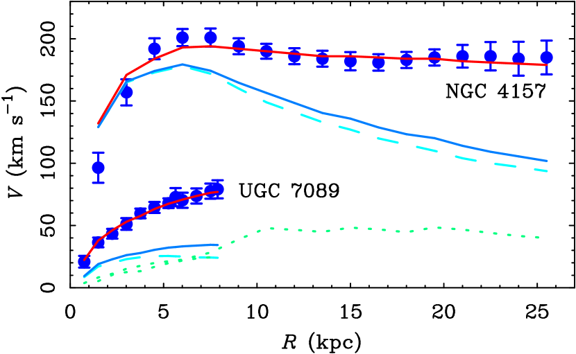
Figure 1: Examples of the data for two galaxies from the study of Sanders & Verheijen (1998). The points with error bars are the measured rotation curves of NGC 4157 and UGC 7089. The dashed lines are the contribution to the rotation by the stars, $V_{\star}(r)$, as determined from $K^{\prime}$-band surface photometry. The dotted lines are the contribution of the gas, $V_{g}(r)$. Note that the gas distributions of these two very different galaxies are rather similar for $r<8$ kpc, so that the dotted lines nearly overlap. The lower solid lines represent the total baryonic contribution, $V_{b}(r)$ (stars plus gas). The upper solid lines are the MOND fits. These are, in effect, a version of $V_{b}(r)$ scaled by the MOND interpolation function $\mu(x)$. Even if MOND is wrong as a theory, this scaling provides an empirical relation between the distribution of observable baryons and that of the dark mass.

Two examples of the data are shown in Fig. 1. The rotation attributable to stars and gas is shown for both galaxies, as is the total rotation due to baryons:

$$V_{b}^{2}=V_{\star}^{2}+V_{g}^{2}.$$ (1)

These components of the velocity are derived from the observed distribution of surface brightness $I(r)$ through numerical inversion of the Poisson equation:

$$\nabla^{2}\Phi_{b}=4\pi G\rho_{b}.$$ (2)

For disks, $\rho_{b}=\Sigma(r)\delta(z)$ where $\Sigma(r)$ is the azimuthally averaged radial surface mass distribution and $\delta(z)$ is the mass distribution perpendicular to the disk. The vertical mass distribution makes little difference to the mass models unless the disk is very thick (axis ratios $<$ 5:1; e.g., de Blok et al. 2003); thin disks are assumed here. A more important factor is the mass-to-light ratio $\Upsilon_{\star}$ which relates the stellar mass distribution to the observed light distribution [$\Sigma(r)=\Upsilon_{\star}I(r)$]. The mass-to-light ratio is assumed to be constant with radius so that the observed distribution of light $I(r)$ specifies the quantity $v_{\star}$: $V_{\star}^{2}(r)=\Upsilon_{\star}v_{\star}^{2}(r)$. (Note that $v_{\star}$ has units $\,\mbox{km}\,\mbox{s}^{-1}\,{\cal M}_{\odot}^{-1/2}\,L_{\odot}^{1/2}$.) The velocity due to the atomic gas component is more directly related to the observed 21 cm flux, with the correction ${\cal M}_{g}=4/3{\cal M}_{\mathrm{HI}}$ for helium and metals. Molecular and ionized gas are assumed to make a negligible contribution to the baryonic mass budget. This is almost certainly fair for ionized gas, and in most cases for molecular gas (e.g., Olling 1996). Molecular gas closely follows the distribution of star light (Regan et al. 2001), so it is subsumed into the stellar mass-to-light ratio.

The centripetal acceleration predicted by Newtonian gravity for the observed baryonic mass components is

$$g_{N}=\frac{V_{b}^{2}}{r}=\left|\frac{\partial\Phi_{b}}{\partial r}\right|.$$ (3)

This is related to the observed centripetal acceleration produced by all mass components

$$a=\frac{V^{2}}{r}=\left|\frac{\partial\Phi}{\partial r}\right|$$ (4)

by MOND through

$$\mu(x)a=g_{N},$$ (5)

where $x=a/a_{0}$ and $a_{0}$ is a constant. The value of $a_{0}$ is taken to be the same in all cases, $a_{0}=1.2\times 10\;{\mathrm{m}}\,{\mathrm{s}}^{-2}$ (Begeman et al. 1991). The interpolation function $\mu(x)$ commonly used in rotation curve fitting is

$$\mu(x)=\frac{x}{\sqrt{1+x^{2}}}$$ (6)

(Milgrom 1983; Sanders & McGaugh 2002). This is effectively just a scaling of the velocity due to the baryonic component. There is a simple formula for mapping $V_{b}(r)$ to the total velocity $V(r)$ (Fig. 1). This procedure has only a single fitting parameter, the stellar mass-to-light ratio $\Upsilon_{\star}$. The physical origin of this scaling aside, the simple fact that it works provides a very useful constraint on the problem.

The MOND procedure has been successfully applied to $\sim 100$ galaxies. Two dozen of these cases have yet to be published (Swaters & Sanders 2004, in preparation), leaving a useful sample of 74 galaxies (Sanders & McGaugh 2002). This is a very large sample for data of this quality and extent.

Though not a complete sample in terms of a survey, this is not important to the purpose here. What is important is coverage of the parameter space over which disk galaxies exist. The sample galaxies cover a large range in rotation velocity ($V_{flat}=50$ to 300$\,\mbox{km}\,\mbox{s}^{-1}$), luminosity ($L_{B}=5\times 10^{7}$ to $2\times 10^{11}L_{\odot}$), scale length ($h=0.5$ to 13 kpc), central surface brightness ($\mu_{0}^{B}=19.6$ to 24.2 mag. arcsec^-2), and gas mass fraction ($f_{g}={\cal M}_{g}/({\cal M}_{\star}+{\cal M}_{g})=0.07$ to 0.95). This range covers most of the parameter space over which disk galaxies are known to reside.

The efficacy of MOND in fitting rotation curves is well established (Sanders & McGaugh 2002). The quality of these fits is illustrated by Figs. 2 and 3, which show the global rms and local velocity residuals of the MOND fits. The rms residuals are small, $<10\%$ in most cases (Fig. 2a). Of course, some data are more accurate than others, so it is interesting to ask how MOND performs as the data improve. To this end, we restrict the sample to include only those points within each galaxy for which the formal uncertainty on the velocity is better than 5%. In crude terms, this is roughly the level at which various astrophysical effects limit one’s knowledge of the true circular velocity (see discussions in McGaugh et al. 2001 and de Blok et al. 2001). This restriction removes the low accuracy points from the rotation curves of individual galaxies, and in 14 galaxies no data remain. The rms residuals improve after the less accurate data are rejected (Fig. 2b): the best data are fit best by MOND.

In the analysis, it is assumed that the orbits being traced are circular. This assumption must fail at some level, causing a deviation of the observed rotation curve from the circular velocity curve of the potential. This effect will usually be most severe at small radii where the gradient in the rotation curve is large, and where the velocity dispersion may contribute significantly to the total kinematic budget, especially in systems with large bulges. The assumption of circular motion will cause the MOND-predicted velocities to exceed the observed ones by a modest amount. This is precisely what is seen in Fig. 3(a), where there is a “beard” of points at small radii with $\Delta V=V-V_{\mathrm{MOND}}<0$. This effect is consistent with the modest amount of non-circular motion one would naturally expect for this sample.

Two galaxies listed by Sanders & McGaugh (2002) are not included here: NGC 3198 and NGC 2841. These galaxies have MOND fits which are sensitive to the distance measurement, as discussed in detail by Bottema et al. (2002). It is not surprising that this should occasionally be an issue since it is acceleration which matters in MOND fits. Since $a=V^{2}/r$, the acceleration can be uncertain (through $r=\theta D$) even if $V$ is well measured. NGC 3198 and NGC 2841 either fall right on target in Fig. 2, and adhere to the same Tully-Fisher and mass discrepancy-acceleration relations as the other 74 galaxies, or they are extreme outliers from these relations, depending on their true distances (and other uncertainties, like the angle of the warp in NGC 2841). If these objects can not be reconciled with MOND, then they constitute a falsification of the theory. Such a situation would not, however, alter any of the conclusions drawn here in the context of dark matter. From this perspective, they would merely be rare cases which deviate from the norm.

3 The Empirical Coupling between Mass and Light

3.1 The Acceleration Scale

From a purely Newtonian perspective, the mass discrepancy in disk galaxies sets in at a particular acceleration scale. Whether this is also true in other systems, especially rich clusters of galaxies, is less clear (Aguirre, Schaye, & Quataert 2001; Sanders 2003), so the discussion here is restricted to rotationally supported disk galaxies. In disks, it is very clear that acceleration is the relevant physical scale (Fig. 4).

The ordinate of Fig. 4 plots the amplitude of the mass discrepancy ${\cal D}$, as quantified by the ratio of the gradient of the total gravitational potential to that of the baryons:

$${\cal D}\equiv\frac{\Phi^{\prime}}{\Phi_{b}^{\prime}}=\frac{V^{2}}{V_{b}^{2}}=\frac{V^{2}}{\Upsilon_{\star}v_{\star}^{2}+V_{g}^{2}}.$$ (7)

In the limit of spherical mass distributions, this is equivalent to the ratio of total to baryonic mass (McGaugh 1999). The mass discrepancy is plotted against several physical scales in Fig. 4: radius, orbital frequency, and centripetal acceleration. The data for all 74 galaxies are plotted together, a total of 1,145 individual resolved velocity measurements.

With so many data from so many different galaxies of such widely varying properties, one might naively expect the result to be a scatter plot. Indeed, this is essentially the case when the mass discrepancy is plotted against radius (top panels of Fig. 4). There are galaxies where the need for dark matter is not apparent until quite large radii, and others in which the mass discrepancy sets in already at small radii. There is no particular radius at which the mass discrepancy always occurs, as we would expect if the rotation curve of the dynamically dominant dark matter $V_{h}(r)$ depends little on the minority baryons.

Much the same is true when the data are plotted against orbital frequency. There is a hint of incipient organization, but there is also still a lot of scatter. Yet when the mass discrepancy is plotted against acceleration, something remarkable happens. All the data from all the galaxies align. The correlation is remarkably strong considering the number of galaxies and independent measurements which went into it.

The baryonic potential computed for Fig. 4, while purely Newtonian, assumes MOND mass-to-light ratios. McGaugh (1999) showed that acceleration is the physical scale with which the mass discrepancy correlates best irrespective of the choice of stellar mass-to-light ratio. However, it is interesting to see how the correlation is affected by other choices of $\Upsilon_{\star}$.

Fig. 5 shows the mass discrepancy-acceleration relation for four choices of stellar mass-to-light ratio ($\Upsilon_{\star}$ in equation 7). Illustrated are maximum disk, MOND, and two choices of stellar population models. The choice labeled “popsynth” computes the mass-to-light ratio from the model of Bell et al. (2003b):

$$\log\Upsilon_{\star}^{B}=1.737(B-V)-0.942$$ (8)

$$\log\Upsilon_{\star}^{K}=0.135(B-V)-0.206$$ (9)

(from their Table 7). “Half popsynth” has the same color dependence, but to emulate a lightweight IMF has its normalization reduced by a factor of two. This is chosen to represent the lower end of the realm of plausibility (Kroupa 2002); reality is presumably bracketed between this and maximum disk. Mass-to-light ratios estimated in this fashion will not be perfect of course, but this does provide a useful estimate for what we expect for stellar populations.

Colors for the galaxies are taken from the original sources where available. In other cases, they are taken from NED, with precedence given to the RC3 (de Vaucouleurs et al. 1995) where available to maximize uniformity. $B-V$ colors were found for 50 of the galaxies; popsynth $\Upsilon_{\star}$ are not computed for the remainder for lack of input to equations 8 and 9.

The mass discrepancy-acceleration relation is clear in Fig. 5 for all choices of mass-to-light ratio. It works nearly as well for maximum disk as it does for MOND mass-to-light ratios. This is because high surface brightness galaxies are close to or in the Newtonian regime ($a\gtrsim a_{0}$) at small radii, so the MOND and maximum disk mass-to-light ratios are similar. The popsynth choice also works well. Individual rotation curves can be perceived in a few cases, but the number of deviant galaxies is small. Only as the mass-to-light ratio becomes implausibly small (half popsynth) does the relation begin to fall apart (as it must in the absurd limit $\Upsilon_{\star}\rightarrow 0$).

The scatter in the mass discrepancy-acceleration relation is minimized for MOND mass-to-light ratios. This is no accident. The trend in the data in this figure is, in effect, the inverse of the MOND interpolation function $\mu(x)$ (equation 6). The MOND mass-to-light ratios have been chosen to minimize the scatter away from this function. Nevertheless, Fig. 5 is a purely Newtonian diagram. We can explicitly fit the data in these diagrams to describe the dependence of the mass discrepancy on acceleration with a function ${\cal D}(x)=\mu^{-1}(x)$ (Fig. 4) or ${\cal D}(y)=\mu^{-1}[\mathrm{g}(y)]\approx\mu^{-1/2}(y)$ (Fig. 5) where $y=g_{N}/a_{0}$. Regardless of how we choose to represent it mathematically, or whether we call it MOND or dark matter, this organization is clearly present in the data.

It seems quite unlikely that this high degree of organization can be an accident. Certainly it can not be a product of bad data. Systematic errors could obscure a real relation, but they can not conspire to give the appearance of one where none exists. Rather, the mass discrepancy-acceleration relation must be a real aspect of nature.

3.2 The Baryonic Tully-Fisher Relation

In addition to the local mass discrepancy-acceleration relation, there also exists the global Tully-Fisher relation. Usually expressed as a relation between luminosity and linewidth, it has long been suspected that this is a manifestation of some more fundamental relation between mass and rotation velocity (e.g., Freeman 1999). McGaugh et al. (2000) explicitly showed that there is indeed a more fundamental relation between the baryonic mass (stars plus gas) and the rotation velocity (see also Bell & de Jong 2001; McGaugh 2003). For galaxies with resolved rotation curves, the velocity in the flat part of the rotation curve, $V_{flat}$, is the obvious quantity of interest, and provides an excellent correlation (Fig. 6).

Fig. 6 illustrates the baryonic Tully-Fisher relation for the same choices of mass-to-light ratio and data accuracy as in Fig. 5. As in Fig. 5, there is a clear correlation in all cases, though it begins to degrade for the half-popsynth case. Also as in Fig. 5, the scatter is minimized for MOND mass-to-light ratios.

Verheijen (1997, 2001) notes that the Tully-Fisher relation for the Ursa Major cluster is remarkably tight, with only barely room for the intrinsic scatter expected from stellar population variations, let alone that expected from halo-to-halo variations. Fig. 6 further emphasizes that whatever physical mechanism underpins the Tully-Fisher relation, it is a remarkably strong one with much less scatter than one would nominally expect (e.g., Eisenstein & Loeb 1996; McGaugh & de Blok 1998a). This tight relation is no surprise if required by the force law. MOND requires a baryonic Tully-Fisher relation of the form

$${\cal M}_{b}={\cal A}V_{flat}^{4}.$$ (10)

A fit to the data in Fig. 6 does indeed find a slope of 4 with a normalization ${\cal A}=50$$\,\mbox{km}^{-4}\,\mbox{s}^{4}\,{\cal M}_{\odot}$. This is somewhat higher than the normalization of McGaugh et al. (2000), though consistent within the uncertainties. The biggest difference is that here I have only used galaxies with $V_{flat}$ explicitly measured from resolved rotation curves as opposed to line widths.

In MOND, the normalization of the baryonic Tully-Fisher relation is ${\cal A}=\chi/(a_{0}G)$, where $\chi$ is a factor of order unity which accounts for the fact that thin disks rotate faster than the equivalent spherical mass distribution. Since the galaxies here have all been fit with $a_{0}=1.2\times 10\;\mathrm{m}\,\mathrm{s}^{-2}$, we measure $<$$\chi$$>$ $=0.79$, as expected (McGaugh & de Blok 1998b). In MOND, the baryonic Tully-Fisher relation should be perfect with no scatter. That there remains a small amount of scatter in Fig. 6 is simply a reflection of the residual uncertainties in the data.

Of the choices of mass-to-light ratio considered here, there is no better choice than MOND for minimizing the scatter in the baryonic Tully-Fisher relation. Maximum disk does a good job, but does less well in this respect because low surface brightness galaxies tend to have very large maximum disk mass-to-light ratios (de Blok & McGaugh 1997; Swaters et al. 2000). This pushes up the scatter as a wide range of mass is inferred at a given luminosity. It also pushes up the normalization at low mass, where most galaxies are of low surface brightness (top panel of Fig. 6). It is only with very high mass-to-light ratios ($\Upsilon_{\star}\gtrsim 10\;{\cal M}_{\odot}/L_{\odot}$) that the stellar mass is significant in these low mass galaxies; in the lower three panels the gas mass dominates the baryonic total and these points do not budge.

Presuming mass is indeed more fundamental than luminosity, one would expect a good choice of population synthesis model mass-to-light ratios to reduce the scatter below that observed in luminosity. That is, a proper matching of $\Upsilon_{\star}$ to each galaxy would remove the component of the scatter due to it. While this does happen with MOND, the popsynth choice does not reduce the scatter (Bell & de Jong 2001), rather increasing it slightly. In retrospect, this is probably due to the fact that one expects a fair amount of scatter in the $\Upsilon_{\star}$-color relation (equations 8 and 9). So while the color may be a good indicator of $\Upsilon_{\star}$ in the mean, when applied to any particular galaxy the scatter simply propagates.

3.3 The Optimal Mass-to-Light Ratio

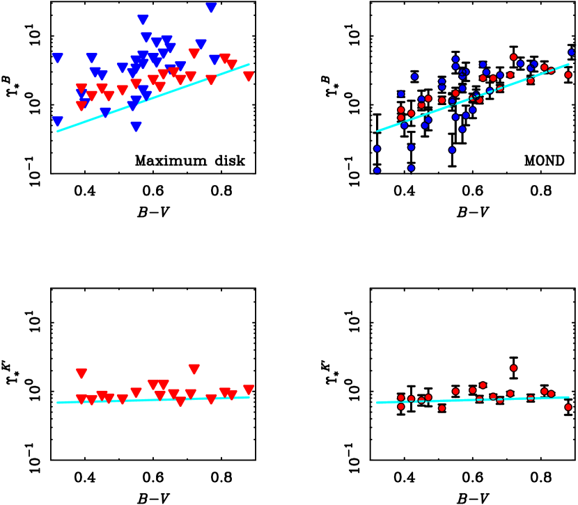
Figure 7: The stellar mass-to-light ratios of disks in the $B$-band (top panels) and $K^{\prime}$-band (bottom panels) as a function of $B-V$ color for the cases of maximum disk (left panels) and MOND (right panels). Each point represents one galaxy for which the requisite data exist. The line represent the mean expectation of stellar population synthesis models from Bell et al. (2003b). These lines are completely independent of the data: neither the normalization nor the slope have been fit to the dynamical data.

Obtaining the mass of a spiral disk is simply a matter of choosing the right mass-to-light ratio. The MOND mass-to-light ratio appears to be optimal, even in a purely Newtonian sense, in that it minimizes the scatter in both the global baryonic Tully-Fisher relation and the local mass discrepancy-acceleration relation. This can be further tested against the expectations of stellar population synthesis models (Fig. 7).

The MOND mass-to-light ratios are in excellent agreement with population synthesis models. These dynamically determined $\Upsilon_{\star}$ are completely independent of the models to which they are compared. Yet they agree well in normalization with the best-guess IMF of Bell & de Jong (2001). In addition, the expected trend of $\Upsilon_{\star}$ with color is apparent. The $K^{\prime}$-band mass-to-light ratio is almost independent of color, while there is a clear trend in the $B$-band for redder galaxies to have higher mass-to-light ratios. The slope of this relation is consistent with the models, and one can even see indications of the turndown in $\Upsilon_{\star}^{B}$ for $B-V<0.5$ apparent in Fig. B1 of Portinari, Sommer-Larsen, & Tantalo (2004). Moreover, the scatter is larger in $B$ than in $K^{\prime}$, again as expected. In this respect, the MOND mass-to-light ratios are more consistent with population synthesis models than popsynth itself, as the latter applies equation 8 or 9 without allowance for the expected scatter.

If we accept the agreement with population models at face value, we can begin to place constraints on the IMF. Bell & de Jong (2001) argue for a “scaled” Salpeter IMF where the best mass-to-light ratio is scaled by a factor ${\cal X}$ from the familiar Salpeter IMF: $\Upsilon_{\star}={\cal X}\Upsilon_{\star}^{\mathrm{Salpeter}}$. By tracing the lower envelope of the maximum disk data of Verheijen (1997) (lower left panel of Fig. 7), Bell & de Jong (2001) argue for ${\cal X}=0.7$. This is a good argument, but one could also argue that one expects a fair amount of scatter about the mean population line, so that a good number of disks should fall below this line even if all disks are maximal. If we take this attitude then ${\cal X}\approx 1.3$ provides a good description of the data. This is not particularly unreasonable from a population perspective, but there are a number of individual galaxies where $\Upsilon_{\star}^{\mathrm{max}}$ is uncomfortably high (typically $\Upsilon_{\star}^{B}\approx 10\,{\cal M}_{\odot}/L_{\odot}$ for blue LSB galaxies).

For the optimal mass-to-light ratios from MOND, ${\cal X}\approx 3/4$. This is in quite good agreement with the detailed investigation of Kroupa & Weidner (2003), who find $0.72<{\cal X}<0.83$ from direct integration of the observed IMF, including brown dwarfs. There is a slight tension between the mean of the $B$ and $K^{\prime}$ bands, in that the $B$-band prefers slightly higher ${\cal X}$. This may be due to residual shortcomings in the models, or may be due to the uncertainty in $\Upsilon_{\star}$ caused by that in the distance to Ursa Major (from whence come all the $K^{\prime}$-band data). The distance determined by Sakai et al. (2000) is rather larger than that of Pierce & Tully (1988), and this cluster is by far the largest outlier from the mean in the Sakai et al. sample. Hence the data still require refinement before a definitive conclusion about the value of ${\cal X}$ can be made. Nevertheless, it is clearly in the right neighborhood, and extreme values, both high and low, can be discounted. For example, ${\cal X}>1.5$ would exceed maximum disk for the majority of $K^{\prime}$-band cases. ${\cal X}<0.35$ (half-popsynth or less) would destroy the correlations which are clear in the data.

There are now three items which point to MOND mass-to-light ratios being optimal in a purely Newtonian sense: (1) they minimize the scatter in the local mass discrepancy-acceleration relation, (2) they minimize the scatter in the global baryonic Tully-Fisher relation, and (3) they could hardly be in better agreement with stellar population models. The obvious conclusion is that these are in fact the correct mass-to-light ratios. This would appear to solve the long standing problem of the uncertainty in disk masses. With the disk mass specified, the dark matter distribution follows.

4 The Dark Matter Distribution

4.1 Constraints on Halo Parameters from the Acceleration Scale

The presence of an acceleration scale in the data provides strong constraints on the parameters of halo models. This follows simply from the observation that there is a point (in Fig. 5) at which the mass discrepancy appears. The constraints discussed here (in §4.1) do not depend on the details of MOND fits or the coupling of mass and light below the critical acceleration scale, but merely upon the fact that there is a critical acceleration scale.

This relevance of the acceleration scale to dark matter halos has been noted by Brada & Milgrom (1999). They pointed out that one can only attribute to dark matter a maximum acceleration not already accounted for by the stars. They demonstrate that there is a formal upper limit to the halo acceleration

$$a^{\mathrm{max}}_{h}\leq\eta a_{\dagger},$$ (11)

where $a_{\dagger}$ is the critical acceleration and $\eta$ is a numerical parameter. For MOND mass-to-light ratios, $a_{\dagger}\ \equiv a_{0}$. The value of $\eta$ depends weakly on the adopted form of the MOND interpolation function, $\mu(x)$. This can be evaluated numerically (see Brada & Milgrom 1999); for the commonly used form of $\mu(x)$ (equation 6) $\eta=0.30$ which I adopt here. The range of $\eta$ spanned by plausible interpolation functions is $0.25\leq\eta\leq 0.37$, so the particular choice of interpolation function is not very important.

Phrasing the constraint in this way makes the relationship to MOND clear. However, the constraint follows simply from the observation that there is an upper limit to the force being provided by the dark halo. We can generalize the MOND result to allow for any choice of mass-to-light ratio. For each choice of $\Upsilon_{\star}$, the effective value of $a_{\dagger}$ can be determined by fitting a function ${\cal D}(y)$ to each panel in Fig. 5. The result is

• for maximum disk: $a_{\dagger}\approx 2300\;{\mathrm{km}^{2}\,\mathrm{s}^{-2}\,\mathrm{kpc}^{-1}}$;

• for popsynth: $a_{\dagger}\approx 4000\;{\mathrm{km}^{2}\,\mathrm{s}^{-2}\,\mathrm{kpc}^{-1}}$; and

• for half popsynth, $a_{\dagger}\approx 10,000\;{\mathrm{km}^{2}\,\mathrm{s}^{-2}\,\mathrm{kpc}^{-1}}$.

The critical acceleration for popsynth is indistinguishable from MOND: $a_{\dagger}\approx a_{0}$. For maximum disk, $a_{\dagger}<a_{0}$, which simply says that the mass discrepancy appears at a somewhat lower acceleration, as should be true by construction. A similar result can be seen in other data (e.g., Palunas & Williams 2000), though the availability of the gas component is necessary for the smooth appearance in Fig. 5. The correlation appears to break down at low accelerations if the gas component is neglected, since it is often the dominant baryonic component at large radii and low accelerations. For half popsynth, $a_{\dagger}>a_{0}$. The fit is still tolerable, but the uncertainty in $a_{\dagger}$ begins to grow large. In the limit $\Upsilon_{\star}\rightarrow 0$, we would of course infer mass discrepancies everywhere, so $a_{\dagger}\rightarrow\infty$.

The scale $a_{\dagger}$ represent an upper limit on the acceleration which can be caused by the dark matter halo. This can be translated to limits on halo parameters for any choice of halo model. These will be rather conservative limits, as we can only require that the maximum acceleration produced by a halo model not exceed $a_{\dagger}$. However, there is no guarantee that the maximum acceleration in any given galaxy will actually occur at the radius of maximum acceleration of a particular halo model. In addition, there is no reason to expect that real galaxies need ever exhibit accelerations as high as $a_{\dagger}$. LSB galaxies have large mass discrepancies precisely because $V^{2}/r<a_{0}$ at all radii. Probably the dominant uncertainty is in the choice of $\Upsilon_{\star}$ and hence the appropriate value of $a_{\dagger}$, though from §3 the most obvious choice is $a_{\dagger}=a_{0}$.

In the following sections, I derive the limits on halo parameters which follow from the acceleration scale limit for the most common halo models. These are the constant density core pseudoisothermal halo and the cuspy NFW halo (Navarro, Frenk, & White 1997). It is straightforward to derive equivalent limits for other choices of halo models, but most other models resemble one of these two in their essential features.

4.1.1 Pseudoisothermal Halos

Traditionally, galaxy rotation curves have been fit with pseudoisothermal halos. These have constant density cores ($\rho=\rho_{c}$) out to a core radius $R_{c}$, after which the profile rolls over to $\rho(r)\rightarrow r^{-2}$ in order to produce asymptotically flat rotation curves. This functional form is very effective at fitting rotation curves, though there is no guarantee that this is what dark matter should do.

The dark matter distribution of the pseudoisothermal halo is

$$\rho_{\mathrm{ISO}}(r)=\frac{\rho_{c}}{1+(r/R_{c})^{2}}$$ (12)

which gives rise to a rotation velocity

$$V_{\mathrm{ISO}}^{2}(r)=V_{f}^{2}\left[1-\frac{R_{c}}{r}\tan^{-1}\left(\frac{r}{R_{c}}\right)\right].$$ (13)

Only two of the parameters $(\rho_{c},R_{c},V_{f})$ are independent, being related by $V_{f}=R_{c}\sqrt{4\pi G\rho_{c}}$. While it is natural to associate $V_{f}$ with the observed $V_{flat}$, this need not be the case in detailed mass decompositions. For nearly maximal disks the baryonic component is often still important at the last measured point, leaving flexibility for $V_{f}\neq V_{flat}$.

The pseudoisothermal halo is a very flexible fitting function, and its parameters are generally not well constrained by direct fits to rotation curves. The fit parameters are highly correlated, particularly $R_{c}$ and $\Upsilon_{\star}$ (Kent 1987). As a result, one can trade one off against the other, leading to the long standing disk-halo degeneracy.

The acceleration constraint helps break this degeneracy. The centripetal acceleration $a_{\mathrm{ISO}}=V_{\mathrm{ISO}}^{2}/r$ due to the halo (equation 13) has a maximum at $r=1.5R_{c}$. The constraint is then

$$a_{\mathrm{ISO}}^{\mathrm{max}}=0.23\frac{V_{f}^{2}}{R_{c}}<\eta a_{\dagger}.$$ (14)

The acceleration constraint is fairly restrictive. For $a_{\dagger}=a_{0}$, small core radii are disallowed for more rapidly rotating galaxies. Small core radii ($R_{c}<1$ kpc) do not occur for typical galaxy velocities ($V_{f}>100$$\,\mbox{km}\,\mbox{s}^{-1}$) unless we invoke implausibly small mass-to-light ratios. Excessive halo velocities ($V_{f}>250$$\,\mbox{km}\,\mbox{s}^{-1}$) are disallowed except for very large core radii ($R_{c}>10$ kpc). This is interesting as it can be quite difficult to constrain $V_{f}$ in many cases where the halo contribution to the velocity is still rising at the last measured point.

4.1.2 NFW Halos

It is not obvious that one expects dark matter halos to be pseudoisothermal. In numerical simulations of structure formation, cold dark matter (CDM) is found to form halos with a rather different structure. For example, Navarro et al. (1997) find that their simulated halos are reasonably well described by

$$\rho_{\mathrm{NFW}}(r)=\frac{\rho_{i}}{(r/R_{s})(1+r/R_{s})^{2}}.$$ (15)

This gives rise to a circular velocity

$$V_{\mathrm{NFW}}^{2}(r)=V_{200}^{2}\left[\frac{\ln(1+cu)-cu/(1+cu)}{u[\ln(1+c)-c/(1+c)]}\right],$$ (16)

where $c=R_{200}/R_{s}$ and $u=r/R_{200}$. $R_{200}$ is the radius which encloses a density 200 times the critical density of the universe (this is, crudely speaking, the virial radius), and $V_{200}$ is the circular velocity of the potential at $R_{200}$.

NFW halos do not have $\rho\propto r^{-2}$ except in transition between two limits, $\rho\propto r^{-1}$ at small radii and $\rho\propto r^{-3}$ at large radii. They do not predict flat rotation curves, which must arise from a combination of disk plus halo. The lack of a constant density core causes problems in fitting the slowly rising rotation curves of dwarf and LSB galaxies (Flores & Primack 1994; Moore 1994; de Blok et al. 2001, 2003; Swaters et al. 2003). In HSB galaxies, some disk mass is required to give flat rotation curves and to avoid excessively high concentrations, but not too much in order to leave room for the central cusp which requires substantial dark mass at small radii.

Maximum disks and NFW halos are mutually exclusive. Even middle-weight disks can significantly modify the primordial halo profile through adiabatic contraction (e.g., Sellwood 1999). We leave an investigation of this point for future work, noting here only that the limits found here will only become stronger after allowance for adiabatic contraction.

The maximum acceleration of an NFW halo occurs at $r=0$. Using equation 16 in the limit $u\rightarrow 0$, the acceleration limit is

$$a_{\mathrm{NFW}}^{\mathrm{max}}=\frac{1}{2}\left[\frac{V_{200}^{2}}{R_{200}}\right]\frac{c^{2}}{\ln(1+c)-c/(1+c)}<\eta a_{\dagger}.$$ (17)

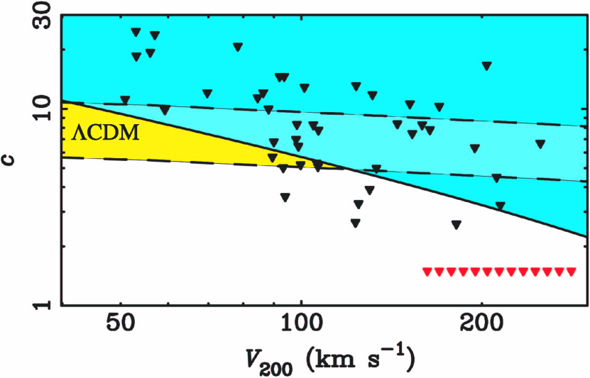
Figure 8: Diagram showing the parameter space of NFW halos. The dashed lines enclose the region in which NFW halos are expected to reside for the cosmological parameters derived from WMAP (Bennett et al. 2003). These lines are drawn for the $\pm 1\sigma$ range of scatter in concentration $\sigma_{c}=0.14$ determined by Weschler et al. (2002). The blue region above the solid line is excluded by the maximum halo acceleration limit $\eta a_{\dagger}$ (Brada & Milgrom 1999). This excludes most of the expected parameter space. Also shown are the upper limits on the concentrations of individual galaxies (points) measured in the limit $\Upsilon_{\star}=0$ by de Blok, McGaugh, & Rubin (2001), de Blok & Bosma (2002), and Swaters et al. (2003). Those objects which would fall outside the boundaries of this plot because of exceedingly low concentrations are plotted as the row of red points at lower right. Individual galaxies need not have halos which achieve the maximum acceleration limit, so such individual cases can be more restrictive (i.e., below the solid line). These are inevitably LSB galaxies with $a<a_{0}$ at all radii.

This can be simplified by noting that $V_{200}=R_{200}h$ (where $h=H_{0}/100{\rm km}\,{\rm s}^{-1}\,{\rm Mpc}^{-1}$). The limit obtained in this fashion is shown in Figure 8. Quite a lot of parameter space is disallowed, including nearly all of that which halos are predicted to occupy by $\Lambda$CDM (Navarro et al. 1997; see also McGaugh, Barker, & de Blok 2003) with the parameters fixed by WMAP (Bennett et al. 2003).

Also shown in Figure 8 are the limits placed by the data for low surface brightness galaxies from de Blok et al. (2003) and Swaters et al. (2003). There is no requirement that all galaxies attain accelerations as high as $a_{\dagger}$, and most of these systems do not. It is for this reason that the limits from some individual galaxies are more restrictive than the limit imposed by equation 17, even when $\Upsilon_{\star}=0$ is assumed.

The data require rather lower halo concentrations than are predicted by $\Lambda$CDM. This holds for all spirals, not just those of low surface brightness. Indeed, NFW halos are more strongly excluded for the high mass halos which we would presumably associate with $L^{\star}$ galaxies than for lower mass dwarfs. The only way to avoid this conclusion is to increase $a_{\dagger}$ by reducing $\Upsilon_{\star}$. The region of parameter space predicted by $\Lambda$CDM is allowed for $a_{\dagger}>10^{4}\;{\mathrm{km}^{2}\,\mathrm{s}^{-2}\,\mathrm{kpc}^{-1}}$. This corresponds to $\Upsilon_{\star}<$ half popsynth (see also Bell et al. 2003a). Stellar mass-to-light ratios this small seem very unlikely considering the large scatter in the mass discrepancy-acceleration relation and baryonic Tully-Fisher relation that they cause (§3).

4.2 A Quantitative Relation Between Dark and Baryonic Mass

The information contained in the data goes well beyond limits on the parameters of simple halo models. The limits discussed in the previous section only make use of the scale $a_{\dagger}$. We can make greater use of the correlation between the mass discrepancy ${\cal D}$ and acceleration. The functional form apparent in Fig. 5 provides a strong constraint on the force produced by the dark matter at all radii.

The observed velocity is the sum, in quadrature, of the various components:

$$V^{2}(r)=V_{\star}^{2}(r)+V_{g}^{2}(r)+V_{h}^{2}(r).$$ (18)

This sum of stars, gas, and dark matter is one valid description of the the observed rotation curve. Another valid description is given by MOND fits:

$$V^{2}(r)=\mu^{-1}(x)\left[\Upsilon_{\star}v_{\star}^{2}(r)+V_{g}^{2}(r)\right].$$ (19)

This is effectively just a scaling of the baryonic component: $V^{2}(r)={\cal D}(x)V_{b}^{2}(r)$. That is, the same relation can be derived in a purely Newtonian fashion from either Fig. 4 or 5 by fitting a function ${\cal D}(x)$ to the bottom panel of Fig. 4 or ${\cal D}(y)$ to Fig. 5. This description is more compact, and depends only on the observed distribution of baryonic mass: the velocity due to the dark matter halo does not explicitly appear. Rather than an arbitrary function of radius $V_{h}(r)$, there is only a single fit parameter ($\Upsilon_{\star}$) which must take a specific numerical value.

Equating these two expressions for $V^{2}(r)$ stipulates what is required of the dark matter halo:

$$V_{h}^{2}(r)=\left[\mu^{-1}(x)-1\right]\left[V_{\star}^{2}(r)+V_{g}^{2}(r)\right].$$ (20)

This equation encapsulates the coupling between mass and light. The observed distribution of baryons is completely predictive of the distribution of dark matter.

There is one, and only one, degree of freedom which is not incorporated in equation 20. It assumes that the MOND mass to light ratios are correct. While this would certainly appear to be the case, we can generalize equation 20 to account for the possibility that the true mass-to-light ratio $\Upsilon_{\star}^{\mathrm{TRUE}}$ differs from the optimal mass-to-light ratio $\Upsilon_{\star}^{\mathrm{MOND}}$. These two mass-to-light ratios are related by

$${\cal Q}\equiv\frac{\Upsilon_{\star}^{\mathrm{TRUE}}}{\Upsilon_{\star}^{\mathrm{MOND}}}.$$ (21)

We can therefore write, with complete generality,

$$V_{h}^{2}(r)=\left[{\cal Q}^{-1}\mu^{-1}(x)-1\right]V_{\star}^{2}(r)+\left[\mu^{-1}(x)-1\right]V_{g}^{2}(r).$$ (22)

This equation makes use of the compact MOND description of rotation curves to specify the distribution of dark matter. It depends not at all on MOND being correct as a theory, but only as a fitting function for rotation curves.

Equation 22 mathematically expresses the strong coupling long noted between mass and light in disk galaxies. It is valid for any choice of mass-to-light ratio, as encapsulated by ${\cal Q}$, the only free parameter. As seen in §3, the most natural value of ${\cal Q}$ is unity. Large deviations from unity will disagree with stellar population constraints, so $V_{h}(r)$ is well constrained.

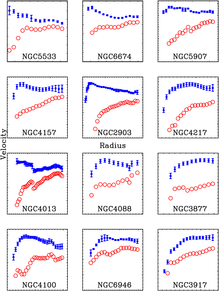
Figure 9: The rotation curves $V(r)$ for individual galaxies with good data (filled points) together with those inferred for the dark matter halo $V_{h}(r)$ after subtraction of the baryonic component (open points). The case of ${\cal Q}=1$ is illustrated here. All plots have (0,0) at the bottom left corner. Tick marks are 1 kpc along the abscissa and 10$\,\mbox{km}\,\mbox{s}^{-1}$ along the ordinate. Galaxies are arranged in order of decreasing velocity, from $V_{\mathrm{max}}\approx 300$$\,\mbox{km}\,\mbox{s}^{-1}$ for NGC 5533 to $V_{\mathrm{max}}\approx 50$$\,\mbox{km}\,\mbox{s}^{-1}$ for DDO 154. There is a wide variety in $V_{h}(r)$, ranging from nearly hollow halos to those that dominate down to small radius.

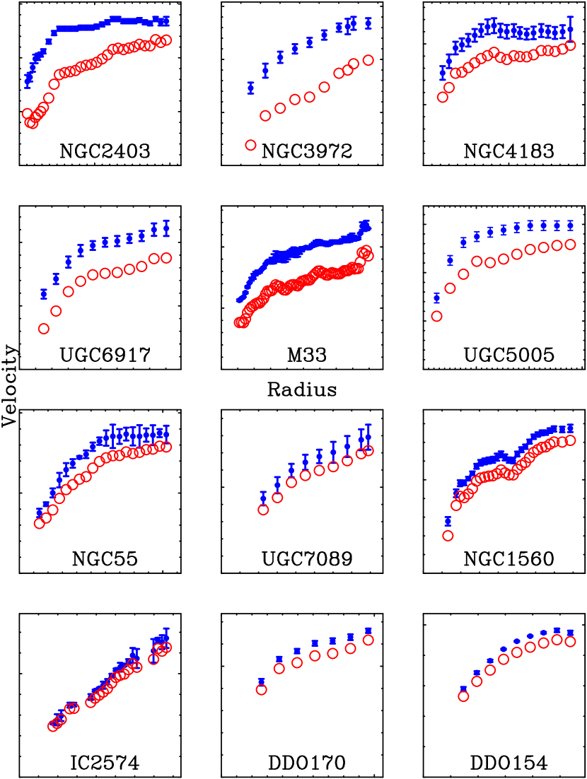
Figure 9: continued.

Some examples of dark matter rotation curves are shown in Fig. 9 for ${\cal Q}=1$. The overall shape of $V_{h}(r)$ is well specified once the baryonic component has been subtracted. Modest deviations from circular motion are probably the cause of some detailed features (e.g., the sharp discontinuity in NGC 4013 which no smooth model can hope to fit) but some other ripples in the inferred dark matter distribution may be real (e.g., the dip in NGC 1560 which is present in the baryonic distribution and reproduced by the MOND fit: Begeman et al. 1991).

The dark matter halos are a mixed bag. Some are dominant at all radii, especially in the dwarf galaxies, while others appear nearly hollow at small radii and never completely dominate even at the last measured point. This occurs for some of the more massive, bulge-dominated systems, reminiscent of the lack of dark matter in the centers of elliptical galaxies (Romanowsky et al. 2003). Overall, it is hard to generalize. Each halo has its own detailed distribution, as unique as that of the baryons which reside within it.

While the overall shape of $V_{h}(r)$ is well specified, it does not follow that model halos fit to these data will be well constrained, even with ${\cal Q}$ held fixed. Models like the pseudoisothermal and NFW halos discussed above have degeneracies between their parameters that can make rather different halos look very similar over a finite range of radii. Observations necessarily span a finite range, and usually only a small fraction of the anticipated virial radius of the halo. Making and interpreting such fits is left for future work, and should be approached with caution.

Having a specific equation for $V_{h}(r)$ is nevertheless of considerable value. Much of the apparent freedom in multi-component mass modeling results from consideration of arbitrary values of ${\cal Q}$ ($0\leq{\cal Q}\leq{\cal Q}_{\mathrm{max}}$) and the degeneracies inherent in halo models. This is a problem with how we analyze the data, not with the data themselves. Indeed, we may be doing ourselves a considerable disservice by trying to force preconceived functional forms upon $V_{h}(r)$, as equation 22 contains more detailed information than can be expressed by simple halo models. Moreover, we do expect some modification of the initial dark matter halo in the process of galaxy formation, so it is not obvious that fitting NFW halos to the current dark mass distribution is even an appropriate procedure. Nevertheless, it remains true (as seen in Fig. 8) that present-day dark matter halos have considerably less mass at small radii than nominally expected for primordial NFW halos.

4.3 A Constraint on Galaxy Formation Models

The halo circular velocity curve $V_{h}(r)$ derived from the mass discrepancy-acceleration relation provides a strong constraint on theories of galaxy formation. For a model to be an acceptable representation of a real galaxy, it must be able to successfully apply equation 22 with ${\cal Q}$ as the only free parameter. That is, one needs to be able to take the detailed distribution of stars and gas in the model and find a plausible value of ${\cal Q}$ which gives $V_{h}(r)$ consistent with that of the model halo.

To qualify for this test, a model must be sophisticated enough to give both a baryonic mass distribution and a rotation curve. The baryonic mass distribution must be more complex than a simple exponential disk; it should reflect the real variation in bulge, stellar disk, and gas disk components. While model dark matter halos have been investigated in great detail, obtaining a robust prediction of the baryonic mass distribution has proven rather more difficult. This depends not only on the details of dissipational collapse, but also on the star formation prescription necessary to distinguish stellar and gaseous components. Models which meet these requirements are only beginning to appear (e.g., Adabi et al. 2003; Zavala et al. 2003; Robertson et al. 2004).

The model of Abadi et al. (2003) provides a good example of the significant hurdles theory still faces. These authors succeed in forming, in a numerical simulation, something which photometrically resembles a real disk plus bulge system. While appealing, this model fails the test posed above. As Abadi et al. (2003) show, the object’s rotation curve is far removed from its photometric equivalent, peaking much too high at a very small radius. To make a proper comparison with data, one needs a large ensemble of such models. Consequently, we are still far away from being able to claim that we have a satisfactory explanation of disk galaxy rotation curves.

Indeed, the particular form of the coupling between baryonic and total mass is rather peculiar. There is no obvious reason to expect such a coupling, let alone one so strong that it can be attributed to a single effective force law which appears to be universal in disks. One can write the equations as above (see also Dunkel 2004), but this merely tells us what is required, not why it happens. By way of analogy, we might just as well suppose that the solar system is really run by an inverse cube law. It just looks like it operates under an effective inverse square law because there is dark matter arranged just so. Such a situation in the solar system would be considered an unacceptable fine-tuning problem. The situation in galaxies is hardly better.

5 Conclusions

There is a strong relation between the distribution of baryonic and total mass in disk galaxies. The shape of the rotation curve predicted by the observed distribution of baryons is homologous to the observed rotation. The mass discrepancy, defined as the ratio of the gradients of the total to baryonic gravitational potential, can be described by a simple function of centripetal acceleration:

$$\Phi^{\prime}/\Phi_{b}^{\prime}={\cal D}(x),$$

where $x=a/a_{0}$ and ${\cal D}(x)$ is the inverse of equation 6. For $a>a_{0}=1.2\times 10^{-10}\;{\rm m}\,{\rm s}^{-2}$, there is no apparent need for dark matter. For $a<a_{0}$, the amount of dark matter increases systematically as acceleration declines.

The empirical organization apparent in the data provides constraints on mass models which have not been considered in traditional disk-halo modeling. Making full use of the information present in the data provides a method for estimating the stellar mass-to-light ratio of spiral disks. These mass-to-light ratios are optimal in that they

• minimize the scatter in the mass discrepancy-acceleration diagram (Fig. 5),

• minimize the scatter in the baryonic Tully-Fisher relation (Fig. 6), and

• are consistent with the expectations of stellar population models (Fig. 7).

Indeed, the mass-to-light ratios are consistent not only with the mean value anticipated for stellar populations, but they also reflect the expected trends with color and the band-pass dependent scatter about the mean color-$\Upsilon_{\star}$ relation. It is hard to imagine that all this could be the case unless these mass-to-light ratios are essentially correct. This appears to solve the long standing problem of the absolute stellar mass of galactic disks.

Once the stellar mass of a disk is fixed, the distribution of dark matter follows. This can be expressed as a simple function of observable quantities:

$$V_{h}^{2}(r)=\left[{\cal Q}^{-1}{\cal D}(x)-1\right]V_{\star}^{2}(r)+\left[{\cal D}(x)-1\right]V_{g}^{2}(r)$$

(equation 22). The dark matter distribution is completely specified by the observed baryonic matter distribution. This presents a serious fine-tuning problem for any theory of galaxy formation.

The only freedom available in the detailed distribution of dark matter inferred from observation is encapsulated in a single parameter ${\cal Q}$. This parameter allows for the unlikely possibility that the actual mass-to-light ratios of stars differs from the optimum value described here. With this limited freedom, the relation derived between baryonic and total mass specifies the dark matter distribution with complete generality.

Explaining how this strong coupling between mass and light arises is a major challenge for galaxy formation theory. All we have done is restate, in a generalized Newtonian fashion, the well-established result that MOND fits rotation curves. The question, of course, is what this means. There are two independent issues here which are often mistakenly conflated. One is the unconventional theory known as MOND. The second is the empirical regularity of the data. If the effective force law apparent in the data is not in fact MOND, then we need to understand how it comes about in the context of dark matter.

The possibilities are limited. Either

• MOND is essentially correct, or

• Dark matter results in MOND-like behavior in disk galaxies.

This is the same conclusion reached by Sanders & Begeman (1994) and McGaugh & de Blok (1998b). The improvement of the data since that time only makes this result more clear.

If dark matter is correct, the tightness of the observed coupling between baryons and dark matter implies a very strong regulatory mechanism. Within the context of dark matter, there seem to be two basic options. Either

• the processes of galaxy formation lead to the observed coupling, or

• there is a direct interaction between dark matter and baryons.

In the first case, some combination of mundane astrophysical effects (e.g., adiabatic contraction, mergers, feedback) are presumed to be the root cause of the coupling. However, no clear mechanism is known which has the required effect. Indeed, it seems extremely unlikely that the chaotic processes of galaxy formation can give such a highly ordered result, much less the finely-tuned coupling between mass and light.

Alternatively, the strong coupling between dynamical and baryonic mass might provide a hint about the nature of the dark matter itself. Rather than interacting with baryons only through gravity, there may be some direct interaction which results in the observed coupling. This amounts to a modification of the nature of the dark matter itself. One obviously wishes to retain the successes of CDM on large scales, but modify it to have the appropriate effect in individual galaxies.

Many modifications of dark matter have been discussed in recent years (e.g., warm dark matter, self-interacting dark matter), motivated at least in part by the difficulties posed by rotation curves. Those proposed modifications which ignore the baryons would not seem to help. It is not adequate to change the dark matter properties in order to insert a soft core in dark matter halos; one must explain equation 22.

A mechanism which provides for the direct connection observed between dark matter and baryons is unknown. Ideas along this line are only now being discussed (e.g., Piazza & Marinoni 2003), so it is too soon to judge whether they are viable. Irrespective of which possibility might seem to hold the most promise, there is clearly some important physics at work which has yet to be understood.

Figure 2: The global rms residuals of MOND rotation curve fits. The radial axis is the magnitude of the residual while the azimuthal angle is assigned randomly to each object to distribute them about the plot. Each point represents one galaxy. In (a), all available data are used, a total of 74 galaxies. In (b), the data are restricted to individual data points within each galaxy with velocities measured to better than 5% accuracy. Fourteen galaxies have no data which satisfy this criterion, leaving 60. For these 60 galaxies, the one parameter MOND fits to the best data are very good.

Figure 3: The local residuals of MOND rotation curve fits. Each point represents one resolved point within each galaxy; the data for all galaxies are shown together. The top panel shows the data for 74 galaxies comprising a total of 1145 independent points. In the bottom panel, the data are restricted to individual data points within each galaxy with velocities measured to better than 5% accuracy, as in Fig. 2. A total of 736 independent points from 60 galaxies survive this cut. The places where the fits are imperfect tend to be where the measurements are least accurate. In general, the quality of the fits improves with the quality of the data.

Figure 4: The mass discrepancy ${\cal D}=V^{2}/V_{b}^{2}$ as a function of various observed scales: radius (top panels); orbital frequency $\Omega=V/r$ (middle panels); and centripetal acceleration $a=V^{2}/r$ (lower panels). In the panels on the left all data are shown; on the right are shown those data with high accuracy ($\sigma_{V}/V<5\%$). Each point represents one resolved point within each galaxy, as in Fig. 3. The horizontal line shows ${\cal D}=1$ where there is no mass discrepancy: baryons suffice to explain the observed motions here. There is a clear organization of the data with respect to acceleration. The mass discrepancy only becomes apparent (${\cal D}>1$) below an acceleration scale of $a_{0}\approx 3700\;{\rm km}^{2}\,{\rm s}^{-2}\,{\rm kpc}^{-1}$

Figure 5: The mass discrepancy as a function of the Newtonian acceleration $g_{N}=V_{b}^{2}/r$ predicted by the observed stars and gas for various choices of mass-to-light ratio. The topmost panels show the result for maximum disk mass-to-light ratios. The second row of panels show the mass-to-light ratios indicated by the $B-V$ colors and the $\Upsilon_{\star}$-color relation from the stellar population models of Bell et al. (2003b). The third row uses the MOND fit mass-to-light ratios (Sanders & McGaugh 2002). The result of adopting a lightweight IMF is illustrated in the bottom row by scaling the population synthesis mass-to-light ratio down by a factor of two. The mass discrepancy is well correlated with the acceleration for any plausible (non-zero) choice of mass-to-light ratio. The rotation curves of a few individual galaxies can be discerned in the population synthesis rows, but the majority of the galaxies are indistinguishable in all cases. The scatter in this local relation is minimized for the MOND mass-to-light ratios, making them optimal in this respect even from a purely Newtonian perspective. The intrinsic scatter of the relation appears to be very small.

Figure 6: The baryonic Tully-Fisher relation for various assumptions about the stellar mass-to-light ratio, as in Fig. 5. The observed baryonic mass of each galaxy, stars plus gas, is plotted against the asymptotic flat rotation velocity. The scatter in this global relation is minimized for MOND mass-to-light ratios. The line fit to this case (${\cal M}_{b}=50V_{flat}^{4}$) is shown in the right panels. In the MOND panel it is shown as a solid line; in the other panels it is shown as a dashed line for reference. Note that colors are only available for 50 of the 74 galaxies, so not all cases appear in the popsynth panels.

References

- (1) Abadi, M.G., Navarro, J.F., Steinmetz, M., & Eke, V.R. 2003, ApJ, 591, 499
- (2) Aguirre, A., Schaye, J., & Quataert, E. 2001, ApJ, 561, 550
- (3) Athanassoula, E., Bosma, A., & Papaioannou, S. 1987, A&A, 179, 23
- (4) Bahcall, J. N. & Casertano, S. 1985, ApJ, 293, L7
- (5) Begeman, K. G. 1987, Ph.D. Thesis, University of Groningen
- (6) Begeman, K. G., Broeils, A. H., & Sanders, R. H. 1991, MNRAS, 249, 523
- (7) Bell, E. F., Baugh, C. M., Cole, S., Frenk, C. S., & Lacey, C. G. 2003a, MNRAS, 343, 367
- (8) Bell, E. F. & de Jong, R. S. 2001, ApJ, 550, 212
- (9) Bell, E. F., McIntosh, D. H., Katz, N., & Weinberg, M. D. 2003b, ApJS, 149, 289
- (10) Bennett, C.L. et al. 2003, ApJS, 148, 1
- (11) Brada, R. & Milgrom, M. 1999, ApJ, 512, L17
- (12) Broeils, A. H. 1992, Ph.D. Thesis, University of Groningen
- (13) Bissantz, N., Englmaier, P., Gerhard, O. 2003, MNRAS, 340, 949
- (14) Bottema, R., Pestaña, J. L. G., Rothberg, B., & Sanders, R. H. 2002, A&A, 393, 453
- (15) Courteau, S. & Rix, H.-W. 1999, ApJ, 513, 561
- (16) Debattista, V. P. & Sellwood, J. A. 1998, ApJ, 493, L5
- (17) Debattista, V. P. & Sellwood, J. A. 2000, ApJ, 543, 704
- (18) de Blok, W.J.G. 1997, Ph.D. Thesis, University of Groningen
- (19) de Blok, W.J.G., & Bosma, A. 2002, A&A, 385, 816
- (20) de Blok, W.J.G., Bosma, A., & McGaugh, S.S. 2003, MNRAS, 340, 657
- (21) de Blok, W.J.G., & McGaugh, S.S. 1996, ApJ, 469, L89
- (22) de Blok, W.J.G., & McGaugh, S.S. 1997, MNRAS, 290, 533
- (23) de Blok, W.J.G., & McGaugh, S.S. 1998, ApJ, 508, 132
- (24) de Blok, W.J.G., McGaugh, S.S., van der Hulst, J.M. 1996, MNRAS, 283, 18
- (25) de Blok, W.J.G., McGaugh, S.S., & Rubin, V.C. 2001, AJ, 122, 2396
- (26) de Vaucouleurs, G., de Vaucouleurs, A., Corwin, H. G., Buta, R. J., Paturel, G., & Fouque, P. 1995, VizieR Online Data Catalog, 7155, 0
- (27) Dunkel, J. 2004, ApJ, 604, L37
- (28) Eisenstein, D. J. & Loeb, A. 1996, ApJ, 459, 432
- (29) Flores, R. A. & Primack, J. R. 1994, ApJ, 427, L1
- (30) Freeman, K. C. 1999, ASP Conf. Ser. 170: The Low Surface Brightness Universe, 3
- (31) Fuchs, B. 2002, Dark matter in astro- and particle physics, 28
- (32) Fuchs, B. 2003a, Identification of Dark Matter, 72
- (33) Fuchs, B. 2003b, Ap&SS, 284, 719
- (34) Hoekstra, H., van Albada, T. S., & Sancisi, R. 2001, MNRAS, 323, 453
- (35) Hoffman, G. L., Salpeter, E. E., Farhat, B., Roos, T., Williams, H., & Helou, G. 1996, ApJS, 105, 269
- (36) Kalnajs, A. J. 1983, in IAU Symp. 100: Internal Kinematics and Dynamics of Galaxies, 109
- (37) Kranz, T., Slyz, A., & Rix, H. 2003, ApJ, 586, 143
- (38) Kroupa P., 2002, Science, 295, 82
- (39) Kroupa, P. & Weidner, C. 2003, ApJ, 598, 1076
- (40) Kent, S.M. 1987, AJ, 94, 306
- (41) McGaugh, S. 1999, ASP Conf. Ser. 182: Galaxy Dynamics - A Rutgers Symposium, 528
- (42) McGaugh, S. 2003, The Mass of Galaxies at Low and High Redshift, 45
- (43) McGaugh, S.S., Barker, M.K, & de Blok, W.J.G. 2003, 584, 566
- (44) McGaugh, S.S., & de Blok, W.J.G. 1998a, ApJ, 499, 41
- (45) McGaugh, S.S., & de Blok, W.J.G. 1998b, ApJ, 499, 66
- (46) McGaugh, S.S., Rubin, V.C., & de Blok, W.J.G. 2001, AJ, 122, 2381
- (47) McGaugh, S. S., Schombert, J. M., Bothun, G. D., & de Blok, W. J. G. 2000, ApJ, 533, L99
- (48) Milgrom, M. 1983, ApJ, 270, 371
- (49) Moore, B. 1994, Nature, 370, 629
- (50) Navarro, J. F., Frenk, C. S., & White, S. D. M. 1997, ApJ, 490, 493
- (51) Olling, R. P. 1996, AJ, 112, 457
- (52) Palunas, P. & Williams, T. B. 2000, AJ, 120, 2884
- (53) Persic, M. & Salucci, P. 1991, ApJ, 368, 60
- (54) Piazza, F., & Marinoni, C. 2003, Phys. Rev. Lett., 91, 141301
- (55) Pierce, M. J., & Tully, B. R. 1988, ApJ, 330, 579
- (56) Portinari, L., Sommer-Larsen, J., & Tantalo, R. 2004, MNRAS, 347, 691
- (57) Regan, M. W., Thornley, M. D., Helfer, T. T., Sheth, K., Wong, T., Vogel, S. N., Blitz, L., & Bock, D. C.-J. 2001, ApJ, 561, 218
- (58) Robertson, B.E., Yoshida, N., Springel, V., & Hernquist, L. 2004, ApJ, 606, 32
- (59) Romanowsky, A. J., Douglas, N. G., Arnaboldi, M., Kuijken, K., Merrifield, M. R., Napolitano, N. R., Capaccioli, M., & Freeman, K. C. 2003, Science, 301, 1696
- (60) Rubin, V. C., Burstein, D., Ford, W. K., & Thonnard, N. 1985, ApJ, 289, 81
- (61) Sancisi, R. 2003, IAU Symposium 220, 192
- (62) Sakai, S. et al. 2000, ApJ, 529, 698
- (63) Sanders, R. H. 1996, ApJ, 473, 117
- (64) Sanders, R.H. 2003, MNRAS, 342, 901
- (65) Sanders, R. H. & Begeman, K. G. 1994, MNRAS, 266, 360
- (66) Sanders, R.H., & McGaugh, S.S. 2002, ARA&A, 40, 263
- (67) Sanders, R. H. & Verheijen, M. A. W. 1998, ApJ, 503, 97
- (68) Sellwood, J. A. 1999, ASP Conf. Ser. 182: Galaxy Dynamics - A Rutgers Symposium, 351
- (69) Sprayberry, D., Bernstein, G. M., Impey, C. D., & Bothun, G. D. 1995, ApJ, 438, 72
- (70) Swaters, R.A., Madore, B.F., & Trewhella, M. 2000, ApJ, 2000, ApJ, 531, L107
- (71) Swaters, R.A., Madore, B. F., van den Bosch, F.C., & Balcells, M. 2003, ApJ, 583, 732
- (72) Swaters, R.A., & Sanders, R.H. 2004, in preparation.
- (73) Tully, R. B. & Fisher, J. R. 1977, A&A, 54, 661
- (74) Tully, R. B. & Verheijen, M. A. W. 1997, ApJ, 484, 145
- (75) Tully, R. B., Verheijen, M. A. W., Pierce, M. J., Huang, J., & Wainscoat, R. J. 1996, AJ, 112, 2471
- (76) van Albada, T. S. & Sancisi, R. 1986, Royal Society of London Philosophical Transactions Series A, 320, 447
- (77) Verheijen, M. A. W. 1997, Ph.D. Thesis, University of Groningen
- (78) Verheijen, M. A. W. 2001, ApJ, 563, 694
- (79) Verheijen, M. A. W. & Sancisi, R. 2001, A&A, 370, 765
- (80) Weiner, B.J., Sellwood, J.A., & Williams, T.B. 2001, ApJ, 546, 931
- (81) Wechsler, R. H., Bullock, J. S., Primack, J. R., Kravtsov, A. V., & Dekel, A. 2002, ApJ, 568, 52
- (82) Zavala, J., Avila-Reese, V., Hernandez-Toledo, H. & Firmani, C. 2003, A&A, 412, 633
- (83) Zwaan, M.A., van der Hulst, J.M., de Blok, W.J.G., & McGaugh, S.S. 1995, MNRAS, 273, L35