A Hubble Space Telescope Lensing Survey of X–ray Luminous Galaxy Clusters: IV. Mass, Structure and Thermodynamics of Cluster Cores at z=0.2

Abstract

We present a comprehensive space–based study of ten X–ray luminous galaxy clusters ($L_{X}{\geq}8{\times}10^{44}{\rm erg\,s^{-1}}$[0.1–2.4 keV]) at $z{=}0.2$. Hubble Space Telescope (HST) observations reveal numerous gravitationally–lensed arcs for which we present four new spectroscopic redshifts, bringing the total to thirteen confirmed arcs in this cluster sample. The confirmed arcs reside in just half of the clusters; we thus obtain a firm lower limit on the fraction of clusters with a central projected mass density exceeding the critical density required for strong–lensing of $50\%$. We combine the multiple–image systems with the weakly–sheared background galaxies to model the total mass distribution in the cluster cores ($R{\leq}500{\rm kpc}$). These models are complemented by high–resolution X–ray data from Chandra and used to develop quantitative criteria to classify the clusters as relaxed or unrelaxed. Formally, $(30{\pm}20)\%$ of the clusters form a homogeneous sub–sample of relaxed clusters; the remaining $(70{\pm}20)\%$ are unrelaxed and are a much more diverse population. Most of the clusters therefore appear to be experiencing a cluster–cluster merger, or relaxing after such an event. We also study the normalization and scatter of scaling relations between cluster mass, luminosity and temperature. The scatter in these relations is dominated by the unrelaxed clusters and is typically ${\sigma}{\simeq}0.4$. Most notably, we detect 2–3 times more scatter in the mass–temperature relation than theoretical simulations and models predict. The observed scatter is also asymmetric – the unrelaxed systems are systematically 40% hotter than the relaxed clusters at 2.5–${\sigma}$ significance. This structural segregation should be a major concern for experiments designed to constrain cosmological parameters using galaxy clusters. Overall our results are consistent with a scenario of cluster–cluster merger induced boosts to cluster X–ray luminosities and temperatures.

1 Introduction

Massive galaxy clusters are the largest collapsed structures in the Universe ($M_{\rm virial}{\simeq}10^{15}{\rm M_{\odot}}$), containing vast quantities of the putative dark matter (DM), hot intracluster gas (${\mathrel{kT_{X}}}{\simeq}7{\rm keV}$), and galaxies ($n_{\rm gal}{\sim}10^{3}$). These rare systems stand at the nodes of the “cosmic web” as defined by the large–scale filamentary structure seen in both galaxy redshift surveys (e.g. de Lapparent, Geller & Huchra 1986; Shectman et al. 1996; Vettolani et al. 1997; Peacock et al. 2001; Zehavi et al. 2002) and numerical simulations of structure formation (e.g. Bond et al. 1996; Yoshida et al. 2001; Evrard et al. 2002). Clusters are inferred to assemble by accreting matter along the filamentary axes, slowly ($t_{\rm crossing}{\sim}2$–3 Gyr) ingesting DM, gas and stars into their deep gravitational potential wells.

Clusters have long been recognized as cosmological probes. For example, the evolution of cluster substructure with look–back–time is in principal a powerful diagnostic of the cosmological parameters (Gunn & Gott 1972; Peebles 1980; Richstone, Loeb & Turner 1992; Evrard et al. 1993). A complementary probe is to constrain the matter density of the universe and the normalization of the matter power spectrum using the cluster mass function. However, it is currently not possible to measure the cluster mass function directly. More easily accessible surrogates such as the X–ray luminosity and temperature functions are therefore used in combination with scaling relations between the relevant quantities (e.g. Eke et al. 1996; Reiprich & Boehringer 2002; Viana, Nichol & Liddle 2002; Allen et al. 2003). A critical component of such analyses is the precision to which the scaling relations are known. Samples of X–ray selected clusters are now of a sufficient size that systematic uncertainties may be comparable with the statistical uncertainties, and therefore deserve careful analysis before robust cosmological conclusions may be drawn (e.g. Smith et al. 2003). Measurements of the Sunyaev–Zeldovich effect (SZE) are also emerging as a powerful cosmological tool (Carlstrom, Holder & Reese 2002). Cosmological SZE surveys will rely on the cluster mass–temperature relationship in a similar manner to cosmological X–ray surveys. Such experiments may therefore also be compromised if astrophysical systematics are identified and carefully eliminated from the analysis (e.g. Majumdar & Mohr 2003). Detailed study of the assembly and relaxation histories of clusters, and their global scaling relations as a function of redshift are therefore vitally important.

To advance our understanding of the assembly, relaxation and thermodynamics of massive galaxy clusters requires information about the spatial distribution of DM, hot gas and galaxies in clusters. Several baryonic mass tracers are available, for example X–ray emission from the intracluster medium (hereafter ICM – e.g. Jones & Forman 1984; Buote & Tsai 1996; Schuecker et al. 2001) and the angular and line–of–sight velocity distribution of cluster galaxies (e.g. Geller & Beers 1982; Dressler & Shectman 1988; West & Bothun 1990). These diagnostics have often been used as surrogates for a direct tracer of the underlying DM distribution. The major drawback of this approach is the requirement to assume a relationship between the luminous and dark matter distributions (e.g. that the ICM is in hydrostatic equilibrium with the DM potential) – it is precisely these assumptions that require detailed testing. This issue is further aggravated by the expectation that cluster mass distributions are DM dominated on all but the smallest scales (e.g. Smith et al. 2001; Sand, Treu & Ellis 2002; Sand et al. 2004).

Gravitational lensing offers a solution to much of this problem, in that the lensing signal is sensitive to the total mass distribution in the lens, regardless of its physical nature and state. Detailed study of gravitational lensing by massive clusters is therefore an important opportunity to gain an empirical understanding of the distribution of DM in clusters. Indeed, early comparisons between X–ray and lensing–based mass measurements revealed a factor 2–3 discrepancy between X–ray and strong–lensing–based cluster mass estimates (e.g. Miralda–Escudé & Babul 1995; Wu & Fang 1997), although the agreement between weak–lensing and X–ray measurements was generally better, albeit within large uncertainties (e.g. Squires et al. 1996, 1997; Smail et al. 1997). The simplifying assumptions involved in the X–ray analysis were soon identified as the likely dominant source of this discrepancy; this was confirmed by several authors (e.g. Allen 1998; Wu et al. 1998; Wu 2000). In summary, X–ray and lensing mass measurements for the most relaxed clusters agree well if the multi–phase nature of the ICM in cool cores (e.g. Allen et al. 2001) is incorporated into the X–ray analysis. The situation is more complex in more dynamically disturbed clusters, with larger discrepancies being found at smaller projected radii. The origin of the X–ray versus lensing mass discrepancy in clusters that do not contain a cool core is generally attributed to the simplifying equilibrium and symmetry assumptions of the X–ray analysis. For that reason, most modern X–ray cluster analyses that involve measuring cluster mass using only X–ray data understandably concentrate on relaxed, cool core clusters (e.g. Allen et al. 2001).

An important caveat to adopting lensing as the tool of choice to measure cluster mass is that lensing actually constrains the projected mass distribution along the line–of–sight to the cluster. The addition of three–dimensional information into lensing studies may therefore be important before final conclusions are drawn. For example Czoske et al.’s (2001; 2002) wide–field redshift survey of Cl 0024$+$1654 at $z{=}0.395$ revealed that this previously presumed relaxed strong–lensing cluster (e.g. Smail et al. 1996; Tyson et al. 1998) cluster is not relaxed, and appears to have suffered a recent merger along the line–of–sight (see also Kneib et al. 2003).

Early gravitational lensing studies of galaxy clusters concentrated on individual clusters selected because of their prominent arcs (e.g. Mellier et al. 1993; Kneib et al. 1994, 1995, 1996; Smail et al. 1995a, 1996; Allen et al. 1996; Tyson et al. 1998). This “prominent arc” selection function was vital to development of the techniques required to interpret the gravitational lensing signal (e.g. Kneib 1993). However it also made it difficult to draw conclusions about galaxy clusters as a population of astrophysical systems from these studies. Smail et al. (1997) used the Hubble Space Telescope (HST) to study a larger sample of optically rich clusters, selected originally for the purpose of studying the cluster galaxies. As X–ray selected samples became available in the late–1990’s, Luppino et al. (1999) also searched for gravitational arcs in ground–based imaging of 38 X–ray luminous clusters. The broad conclusions to emerge from these pioneering studies were that to use gravitational lensing to learn about clusters as a population, a selection function that mimics mass–selection as closely as possible, and the high spatial resolution available from HST imaging are both key requirements.

We are conducting an HST survey of an objectively selected sample of ten X–ray luminous (and thus massive) clusters at $z{\simeq}0.2$ (Table 1, §2). Previous papers in this series have presented (i) a detailed analysis of the density profile of A 383 (Smith et al. 2001), (ii) a search for gravitationally–lensed Extremely Red Objects (EROs – Smith et al. 2002a) and (iii) near–infrared (NIR) spectroscopy of ERO J003707, a multiply–imaged ERO at $z{=}1.6$ behind the foreground cluster A 68 (Smith et al. 2002b). This paper describes the gravitational lensing analysis of all ten clusters observed with HST and uses the resulting models of the cluster cores to measure the mass and structure of the clusters on scales of $R{\leq}500\,{\rm kpc}$. We also exploit archival Chandra observations and NIR photometry of likely cluster galaxies to compare the distribution of total mass in the clusters with the gaseous and stellar components respectively. This combination of strong–lensing, X–ray and NIR diagnostics enable us to quantify the prevalence of dynamical immaturity in the X–ray luminous population at $z{\simeq}0.2$ and to calibrate the high–mass end of the cluster mass–temperature relationship.

We outline the organization of the paper. In §2 we describe the survey design and sample selection. We then describe the reduction and analysis of the optical data in §3, comprising the HST imaging data (§3.1) and new spectroscopic redshift measurements for arcs in A 68 and A 2219 (§3.2). The end–point of §3 is a definition of the strong– and weak–lensing constraints available for all ten clusters. We apply these constraints in §4, to construct detailed gravitational lens models of the cluster potential wells; the details of the modelling techniques are described in the Appendix, and the process of fitting the constraints in each cluster are described in §4. We then complement these gravitational lensing results with observations of the X–ray emission from the clusters’ ICM, drawn from the Chandra data archive (§5). The main results of the paper are then presented in §6, including measurements of the mass and maturity of the clusters and a detailed study of the cluster scaling relations. We discuss the interpretation of the results in §7 and briefly assess their impact on attempts to use clusters as cosmological probes. Finally, we summarize our conclusions in §8

We assume a spatially flat universe with $H_{0}{=}50{\rm km\,s^{-1}Mpc^{{-}1}}$ and $q_{0}{=}0.5$; in this cosmology $1^{\prime\prime}{\equiv}4.2\,{\rm kpc}$ at $z{=}0.2$. Our main results are insensitive to this choice of cosmology, for example, the cluster mass measurements would be modified by ${\mathrel{\hbox{\hbox to0.0pt{\hbox{\lower 4.0pt\hbox{$\sim$}}\hss}\hbox{$<$}}}}10\%$ if we adopted the currently favored values of $\Omega_{\rm M}{=}0.3$, $\Omega_{\Lambda}{=}0.7$, $H_{0}{=}65{\rm km\,s^{-1}Mpc^{{-}1}}$. We also adopt the complex deformation, $\vec{\tau}{=}\tau_{x}{+}i\tau_{y}{=}|\vec{\tau}|e^{2i\theta}$, as our measure of galaxy shape when dealing with the weak lensing aspects of our analysis, where $\tau{=}(a^{2}{+}b^{2})/2ab$ and $\theta$ is the position angle of the major axis of the ellipse that describes each galaxy. We define the terms “ellipticity” to mean $\tau$ and “orientation” to mean $\theta$. All uncertainties are quoted at the 68% confidence level.

2 Sample Selection

Table 1: Summary of Hubble Space Telescope Observations

Cluster	Central Galaxy	$z$	$\mathrel{L_{X}}^{a}$	$\mathrel{T_{\rm exp}}$
	$\alpha,\delta$ (J2000)			(ks)
A 68	00 37 06.81 ${+}$09 09 24.0	0.255	$8.4{\pm}2.3$	$7.5$
A 209	01 31 52.53 ${-}$13 36 40.5	0.209	$15.2{\pm}1.0$	$7.8$
A 267	01 52 41.97 ${+}$01 00 26.2	0.230	$11.1{\pm}0.9$	$7.5$
A 383	02 48 03.38 ${-}$03 31 45.7	0.187	$9.8{\pm}0.3$	$7.5$
A 773	09 17 53.37 ${+}$51 43 37.2	0.217	$12.5{\pm}2.1$	$7.2$
A 963	10 17 03.57 ${+}$39 02 49.2	0.206	$13.4{\pm}1.0$	$7.8$
A 1763	13 35 20.10 ${+}$41 00 04.0	0.228	$14.2{\pm}2.1$	$7.8$
A 1835	14 01 02.05 ${+}$02 52 42.3	0.253	$38.3{\pm}0.9$	$7.5$
A 2218	16 35 49.22 ${+}$66 12 44.8	0.171	$9.0{\pm}0.8$	$6.5$
A 2219	16 40 19.82 ${+}$46 42 41.5	0.228	$19.8{\pm}2.2$	$14.4$

a ${\mathrel{L_{X}}}$ is given in the [0.2–2.4 keV] pass–band in units of $10^{44}\,{\rm erg\,s^{{-}1}}$. Luminosities are taken from XBACs catalog (Ebeling et al. 1996) unless measurements based on pointed observations are available: A 383, Smith et al. (2001); A 209, A 267, A 963, A 1835, Allen et al. (2003).

We aim to study massive galaxy clusters, and so would prefer to select clusters based on their mass. Mass–selected cluster catalogs extracted from ground–based observations are gradually becoming available (e.g. Miyazaki et al. 2002; Wittman et al. 2003), however the blurring effect of the atmosphere make the completeness of these weak–lensing cluster catalogs very difficult to characterize robustly. These surveys are also unlikely to achieve the sky coverage (of order full–sky) required to detect a large sample of the rarest and most massive systems which are the focus of our program. In contrast, X–ray selected cluster catalogs (e.g. Gioia et al. 1990; Ebeling et al. 1998, 2000; De Grandi et al. 1999) based on the ROSAT All–Sky Survey are already available in the public domain with well–defined completeness limits. X–ray selection also influences the choice of survey epoch because the completeness of the X–ray cluster catalogs at the time that we applied for HST time in Cycle 8 (GO–8249) fell off rapidly beyond $z{\simeq}0.3$. We therefore adopt $z{=}0.2$ as the nominal redshift of our cluster sample. This redshift is also well–suited to a lensing survey because the observer–lens, observer–source and lens–source angular diameter distances ($\mathrel{D_{\rm OL}},\mathrel{D_{\rm OS}},\mathrel{D_{\rm LS}}$) that control the power and efficiency of gravitational lenses render clusters at $z{\simeq}0.2$ powerful lenses for background galaxy populations at $z{\sim}0.7$–1.5. This redshift interval is well–matched to the current generation of optical spectrographs on 10–m class telescopes.

Accordingly, we select ten of the most X–ray luminous clusters ($L_{X}{\geq}8{\times}10^{44}\,{\rm ergs\,s^{-1}}$, 0.1–2.4 keV) in a narrow redshift slice at $0.17{\leq}z{\leq}0.25$, with minimal line–of–sight reddening ($E(B{-}V){\leq}0.1$) from the XBACs sample (X–ray Brightest Abell–type Clusters; Ebeling et al. 1996). These clusters span the full range of X–ray properties (morphology, central galaxy line emission, cooling flow rate, core radius) found in larger X–ray luminous samples (e.g. Peres et al. 1998; Crawford et al. 1999). The median X–ray luminosity of the sample is $13{\times}10^{44}{\rm erg\,s^{-1}}$. We list the cluster sample in Table 1. As XBACs is restricted to Abell clusters (Abell, Corwin, & Olowin 1989), the sample is not strictly X–ray selected. However, a comparison with the X–ray selected ROSAT Brightest Cluster Sample (BCS; Ebeling et al. 1998, 2000a) shows that 18 of the 19 BCS clusters that satisfy our selection criteria are either Abell or Zwicky clusters. This confirms that our sample is indistinguishable from a genuinely X–ray selected sample.

3 Optical Data and Analysis

3.1 HST Observations and Data Reduction

All ten clusters were observed through the F702W filter using the WFPC2 camera on board HST. The total exposure time for each cluster is listed in Table 1. We adopted a three–point dither pattern for the eight clusters (A 68, A 209, A 267, A 383, A 773, A 963, A 1763, A 1835) observed in Cycle 8: each exposure was shifted relative to the previous one by ten WFC pixels (${\sim}1.0^{\prime\prime}$) in $x$ and $y$. The archival observations of A 2218 follow the same dither pattern, except the offsets were three WFC pixels in $x$ and $y$. A 2219 was observed with a six–point dither pattern that comprised two three–point dithers each of which were identical to that used for the Cycle 8 observations. These two dither patterns were offset from each other by 10 pixels in $x$ and $y$.

We measure the actual dither pattern and compare it with the commanded integer pixel offsets; the median difference between the commanded and actual offsets is $0.2$ pixels, and generally lies in the range ${\sim}0$ – $0.4$ pixels. The geometrical distortion at the edge of each chip (Gilmozzi et al. 1995; Holtzmann et al. 1995; Trauger et al. 1995; Casertano & Wiggs 2001) translates to an additional ${\sim}0.2$ pixel shift at the edge of each detector, falling to zero at the chip centers. Our observations therefore sub–sample the $0.1^{\prime\prime}$ WFC pixels at a level that varies spatially in the range ${\sim}0$ – $0.5$ pixels. We therefore use the dither package (Fruchter & Hook 2002) to reduce the HST data because this allows us to correct for the geometrical distortion and to recover a limited amount of spatial information from the under–sampled WFPC2 point spread function (PSF). The final reduced frames (Fig. 1) have a pixel scale of $0.05^{\prime\prime}$ and an effective resolution of FWHM${=}0.17^{\prime\prime}$.

       

       

       

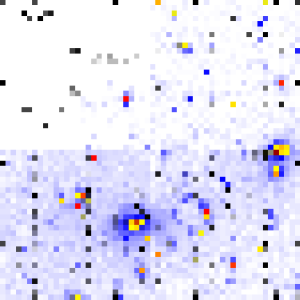
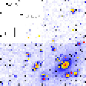
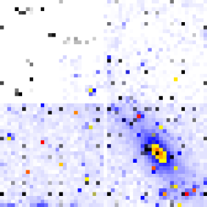
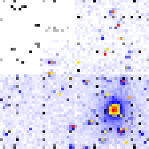
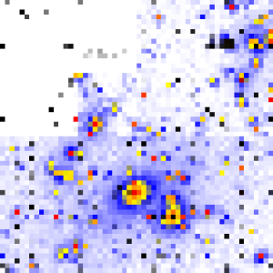
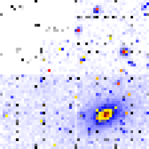
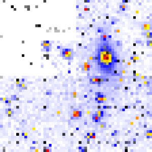
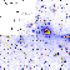
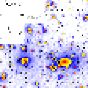
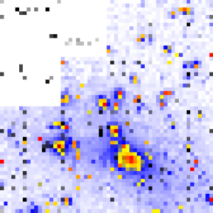
Figure 1: The HST/WFPC2 frames of all ten clusters on a logarithmic scale and a false colour table. We overplot the weak shear field; these vectors show the mean ellipticity and orientation of faint background field galaxies on a grid that has been smoothed with a Gaussian of $\sigma{=}10^{\prime\prime}$. The tickmarks are centered on the central galaxy (Table 1) and are separated by $10^{\prime\prime}$.

3.2 Identification and Confirmation of Multiple–image Candidates

The primary reason for observing the cluster cores with HST is to take advantage of the exquisite spatial resolution of these data to identify multiply–imaged galaxies. Spectroscopic confirmation of such systems provides very tight constraints on the absolute mass of each cluster (roughly an order of magnitude better than is available from weak–lensing), and the spatial distribution of the cluster mass.

We therefore begin the analysis by searching the HST frames for candidate multiple–image systems. This search combines visual inspection of the data (looking for symmetric image pairs and tangentially or radially distorted arcs) with the SExtractor source catalogs described in §3.3. The effective surface brightness limit of the search in regions not affected by bright cluster galaxies is therefore $\mu_{702}{\simeq}25$ mag arcsec^-2 (§3.3). To overcome the influence of bright cluster members, we generated unsharp–masked versions of the science frames, thus removing most of the flux from the bright galaxies. For example this exercise helped us to identify C19 under the brightest cluster galaxy (BCG) in A 68 (Fig. 2). The residual light from the bright galaxies in these unsharp–masked frames inevitably brightens the surface–brightness limit of the multiple–image search close to the cores (central few arcsec) of the subtracted galaxies. However, the only images that we expect to find in such locations are strongly de–amplified counter–images, the brighter images of which should be easily detectable elsewhere in the frame, if they lie above the surface brightness detection limit. We therefore expect the search for multiple–image systems to be reasonably complete to $\mu_{702}{\simeq}25$ mag arcsec^-2.

We list the multiple–image candidates in Table 2, and mark them in Fig. 2. Faint sources detected in the cluster cores are excluded from Table 2 if they are not plausibly multiply–imaged, based on morphological grounds, including examination of issues relating to the parity of possible counter images (see Smith 2002 for a more detailed discussion of issues relating to the identification of multiple–image candidates). The clusters are sub–divided in Table 2 into those with spectroscopically confirmed multiple–image systems (top) and those for which no spectroscopic identifications of genuine multiple–image systems is yet available (bottom). Each sub–set of clusters contains half of the total sample of 10. Of the five clusters without any spectroscopically confirmed multiples, two contain convincing strong–lensing candidates: A 267 (E2) and A 1835 (K3). A firm lower limit on the fraction of clusters in this sample that contain a core region with a projected mass density above the critical density required for strong–lensing is therefore 50%, although values as high as ${\sim}$70–80% are also plausible.

Table 2 also lists the spectroscopic redshifts that are available from other articles in this series (Smith et al. 2001, 2002b), and the published literature. We refer the interested reader to these articles for the details of the spectroscopy and multiple–image interpretation. Note that some of the previously published multiple–image identifications were based on ground–based data, and therefore suffered from quite severe uncertainties. We discuss in §4 improvements to the interpretation of the data that are now possible using the HST data presented here. We also present below new spectroscopic identifications of four multiple–image candidates, recently obtained with the Keck and Subaru telescopes.

Table 2: Multiple–image Candidates and Spectroscopic Redshifts

Cluster	Candidate	Redshifta	References	Notes	Also known as
Clusters with Spectroscopically Confirmed Multiple–images [5/10]
A 68	C0a/b/c	$1.60$	1,2	Triply–imaged ERO	EROJ 003707
	C1a/b/c	$2.6{\pm}0.3$
	C2a/b	$1.5{\pm}0.3$		Faint image pair; counter–image not detected
	C4	$2.625$	§3.2	Ly–$\alpha$ in emission. Singly imaged?
	C6/C20	$4{\pm}0.5$		Pair of images (C6) plus counter image (C20)
	C8	$0.861$	3	Singly imaged?
	C12	$1.265$	3	Singly imaged?
	C14	$0.623$	3	Singly imaged?
	C15/C16/C17	$5.4$	4	Ly–$\alpha$ emitter.
	C19			Possible radial counter images of part of C0
A 383b	B0/B1/B4	$1.010$	5,6	Radial and tangential arc system
	B2a/b/c/d/e	$3{\pm}0.5$	5
	B3a/b/c	$3{\pm}0.5$	5
	B17	$3{\pm}0.5$	5
	B18	$0.656$	5
A 963	H0	$0.771$	7	Three merging images.	“Northern” arc
	H1/H2/H3	$1{\pm}0.5$	7	Group of singly–imaged galaxies?	“Southern” arc
	H6	$3.269$	3	Singly–imaged?
	H7/H8	$0.731$	3	Two singly–imaged galaxies.
A 2218c	M0a/b/c/d/e	$0.702$	8		#359/328/337/389
	M1a/b/c	$2.515$	9		#384/468
	M2a/b	$5.576$	10	Ly–$\alpha$ emitter
	M3a/b/c	$1.1{\pm}0.1$	11		#444/H6
	M4	$1.034$	8,12		#289
A 2219	P0	$1.070$	13,14,§3.2	[oii] in emission; merging pair of images	${\rm N_{12}}$
	P1			Disk galaxy; edge of disk is counter image of P0	${\rm N_{3}}$
	P2a/b/c	$2.730$	13,14,§3.2		${\rm L_{123}}$
	P3/P4	$3.666$	14,§3.2		A, C
	P5		14,§3.2	Counter image of P3/P4	B
	P6/P7/P8	$2.5{\pm}0.2$		Faint pair (P6/P7) plus counter–image (P8)
	P9/P10	$1.3{\pm}0.2$		Candidate pair adjacent to P0
	P11/P12	$1.5{\pm}0.3$		Faint pair
Clusters with only Candidate Multiple–images [5/10]
A 209	D0			Faint arclet – singly imaged?
	D1			Asymmetric morphology – singly imaged?
	D2			Disturbed morphology – singly imaged?
A 267	E1	$0.23$	15	Cluster member
	E2a/b			Faint image pair; counter–image not detected.
A 773	F0	$0.650$	3	Singly–imaged?
	F13	$0.398$	3	Singly–imaged?
	F18	$0.487$	3	Singly–imaged?
	F19	$0.425$	3	Singly–imaged?
A 1763	J4		1	Singly imaged or merging pair?	EROJ 133521+4100.4
A 1835	K0		16	Radial feature – associated with BCG?	A 1835–B′
	K1		16	High surface brightness arclet – singly–imaged?	A 1835–B
	K2			Faint arclet – singly imaged?
	K3		16	Low surface brightness blue arcs	A 1835–A

a Redshift stated with an error bar are inferred from the lens model of the relevant cluster.

b See Smith et al. (2001) for a full list of candidate multiples in A 383.

c See Kneib et al. (1996; 2004, in prep.) for a full list of candidate multiples in A 2218.

References [1] Smith et al. (2002a), [2] Smith et al. (2002b), [3] Richard et al. (2003, in prep.), [4] Kneib et al. (2004a, in prep.), [5] Smith et al. (2001), [6] Sand et al. (2004), [7] Ellis et al. (1991), [8] Pelló et al. (1992), [9] Ebbels et al. (1998), [10] Ellis et al. (2001), [11] Kneib et al. (1996), [12] Swinbank et al. (2003), [13] Smail et al. (1995), [14] Bézecourt et al. (2000), [15] Kneib et al. (2004b, in prep.), [16] Schmidt, Allen & Fabian (2001),

     

     

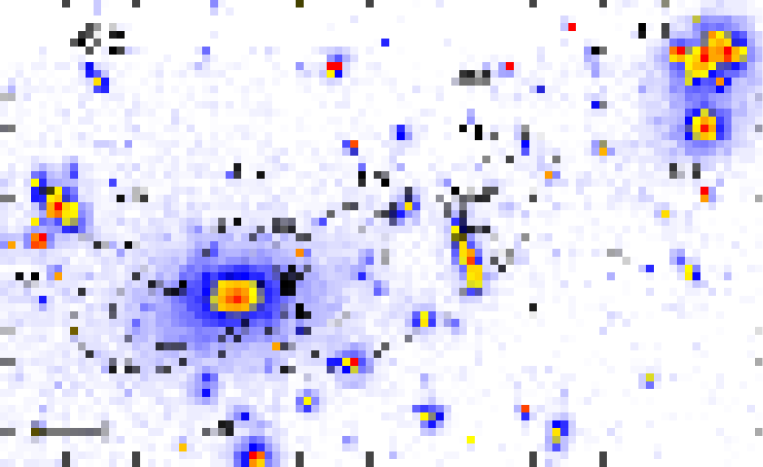
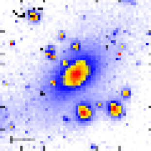
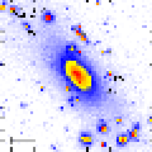
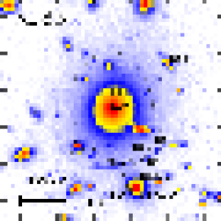
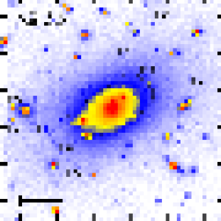
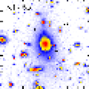
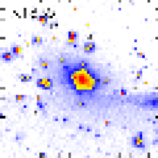
Figure 2: Zooms into the central region of seven of the clusters showing the confirmed and candidate multiple–image systems discussed in the text. The black curves follow the $z{=}1.60,5.4$, $z{=}1.01$ and $z{=}0.771$ tangential critical curves for A 68, A 383 and A 963 respectively as computed from the lens models. The bar at the bottom left of each panel shows a physical scale of 50 kpc. The orientation of each panel matches the corresponding panel in Fig. 1; tick marks are spaced at $5^{\prime\prime}$ intervals.

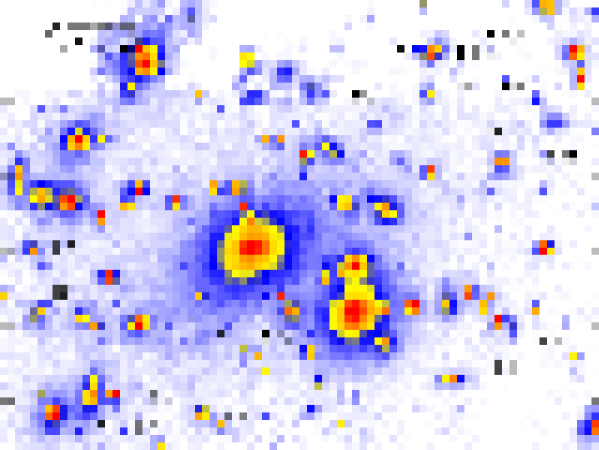
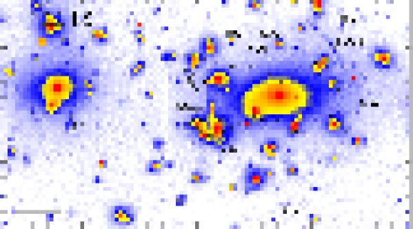
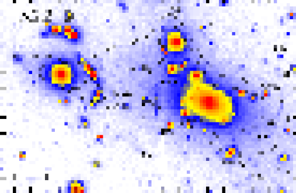
Figure 2: [continued] Zooms into the central region of A 773, A 2218 and A 2219, showing the confirmed and candidate multiple–image systems discussed in the text. The curves follow the $z{=}0.702$ and $z{=}1.069,3.666$ tangential critical curves for A 2218 and A 2219 respectively, as computed from the lens models. The bar at the bottom left of each panel shows a physical scale of 50 kpc. The orientation of each panel matches the corresponding panel in Fig. 1; tick marks are spaced at $5^{\prime\prime}$ intervals.

3.2.1 Keck–I/LRIS Observations of A 68

Figure 3: One–dimensional spectrum of C4 in A 68, obtained with LRIS. We interpret the single strong emission line as Ly–$\alpha$ at $z{=}2.625$ (see §3.2 for more details).

On November 30, 2002, we conducted deep multi–slit spectroscopy with the Low Resolution Imager Spectrograph (LRIS; Oke et al 1995) on the Keck–I telescope, on the cluster A 68. The night had reasonable seeing, ${\sim}0.8^{\prime\prime}$, but was not photometric (with some cirrus), thus no spectrophotometric standard stars were observed. A 68 was observed for a total of 7.2 ks using the D680 dichroic with the 600/7500 grating on the red side and the 400/3400 grism on the blue side. On the red side the spectral dispersion was 1.28Å pixel^-1 with a spatial resolution of 0.214″ pixel^-1, and on the blue side, the spectral dispersion was 1.09Å pixel^-1 with a spatial resolution of 0.135″ pixel^-1 using the blue sensitive 2k${\times}$4k Marconi CCDs.

           

Figure 4: One–dimensional spectra of P0 (left), P2c (center) and P3 (right) multiple–image systems in A 2219, obtained with the FOCAS spectrograph on Subaru. The vertical dotted lines in each panel mark the features used to identify the redshift of each system; the details of these identifications is discussed in §3.2.

Three multiple–image candidates were targetted in the mask: C0ab, C1c and C4 (Table 2). Only C4 has a strong spectral feature – a single strong emission line at ${\mathrel{\lambda_{\rm obs}}}{=}4404.7$ Å (Fig. 3). We interpret this line as Ly–$\alpha$ ${\lambda}$1216Å at $z{=}2.625$. The only other possibility would be [oii] at $z{=}0.18$, i.e. in front of the cluster. We consider this the less likely option given the apparent tangential distortion of the arclet with respect to the cluster center, and the presence of C3 and C20 which appear to be lensed galaxies at a similar redshift to C4 (Fig. 2). We note however, that it appears these three arclets are each single images of different background galaxies.

3.2.2 Subaru/FOCAS Observations of A 2219

On May 29–30, 2001, we conducted deep multi–slit spectroscopy of A 2219 with the Faint Object Camera And Spectrograph (FOCAS; Kashikawa et al 2002) on the Subaru 8.3–m telescope. The two nights had reasonable seeing, ${\rm FWHM}{\simeq}0.8^{\prime\prime}$, but were not fully photometric (with some cirrus), nevertheless we obtained a crude flux calibration using the spectrophotometric standard star “Wolf1346”.

We observed A 2219 for a total of 12.6 ks using the Medium Blue (300B/mm) grism and the order sorting filter Y47. We used the MIT 2k$\times$4k CCD detector with a binning factor of 3 in $x$ and 2 in $y$, this gives us a spectral dispersion of 2.8Å pixel^-1 and a spatial resolution of 0.3″ pixel^-1. Four multiple image candidates were targetted in the mask: P0 and P2c had previously been identified by Smail et al. (1995) as gravitational arcs, and P3/P4 had been identified by Bézecourt et al. (2000) as lying at $z{=}3.6{\pm}0.4$ using photometric redshift techniques. We list the results of our observations (see also Figure 4):

• P0 is identified as a $z{=}1.069{\pm}0.001$ star–forming galaxy showing a strong [oii] $\lambda$3727Å emission plus weak Balmer and Calcium lines.

• P2c is identified as a $z{=}2.730{\pm}0.001$ galaxy using the following interstellar metal absorption lines: OI $\lambda$1302.17Å, SiIV $\lambda$1393.7, 1397.0Å, FeII $\lambda$1608.45Å, CI $\lambda$1656.93Å, and AlII $\lambda$1670.79Å.

• P3 is identified as a $z{=}3.666{\pm}0.001$ galaxy using a broad Ly–$\alpha$ absorption feature and the metal absorption lines OI $\lambda$1302.17Å, SiIV $\lambda$1393.7, 1397.0Å, plus CIV $\lambda$1548.2, 1550.77Å in emission with a broad absorption feature on the blue side.

• P4 was also observed, although, it appears that the slit was not well aligned with the target galaxy, possibly due to a mask–milling problem. We do however detect an absorption feature in these data at the same wavelength as the Ly–$\alpha$ absorption feature in P3. It therefore appears that P4 is also at $z{=}3.666$.

We interpret P0 as a pair of merging images straddling the $z{=}1.07$ critical line. Smail et al. (1995) proposed that P1 is the counter–image of this pair, however Bézecourt et al. (2000) argued against P1 because its optical/near–infrared colours are redder than those of P0. When constraining the lens model of this cluster with just this multiple–image system, several alternative counter–images provided plausible fits. However when this constraint was combined with other multiple–image systems, especially P3/P4/P5 which also lies in the saddle region between the BCG and the group of galaxies to the South–West, an acceptable model was only possible if P1 is identified as the counter–image of P0. The contradiction between this result and Bézecourt et al.’s (2000) photometry is eliminated by the superb spatial resolution of the HST data, because it reveals that P1 is a disk galaxy, the Southern portion (presumably part of the disk) of which has a surface–brightness consistent with that of P0. This is confirmed by inspection of a colour image of this field based on Czoske’s (2002) $BRI$–band CFH12k imaging of this cluster, which reveals that the Southern envelope of P1 is also bluer than the central region, and is consistent with this interpretation.

The spectroscopic identifications of P3 and P4 confirm Bézecourt et al.’s (2000) results. We identify P5 as the third image of this galaxy.

3.3 Source Extraction and Analysis

In addition to the multiple–image constraints described in the previous section, we also need to construct catalogs of cluster galaxies and faint, weakly lensed galaxies. The former are incorporated into the gravitational lens models (§4) as galaxy–scale perturbations to the overall cluster potential. The latter supplement the multiple–image systems to further constrain the parameters of the lens models.

         

Figure 5: left — Mean tangential shear, $\tau_{\rm u,raw}$, of the high signal–to–noise star sample as a function of radial distance from the stacked chip center. The dashed line shows the polynomial fit to these data that we used to remove the PSF anisotropy. right — The results of Monte Carlo simulations to test how accurately we can measure the ellipticity of faint galaxies. The measured ellipticity as a fraction of the true ellipticity is well–fitted by a second–order polynomial function (dashed curve). When the galaxy image is smaller than ${\sim}30$ pixels, the shape measurements are overwhelmed by the PSF and the effects of pixelization. We therefore cut our faint galaxy catalogs at a “faint” limit of area${\geq}30$ pixels. We also use the polynomial function plotted in this figure to correct the observed ellipticities to intrinsic ellipticities.

The first step toward the cluster and background galaxy catalogs is to analyze the HST frames using SExtractor (Bertin & Arnouts 1996). We selected all objects with isophotal areas in excess of $7$ pixels ($0.017$ arcsec²) at the $\mu_{702}{=}25.2$ mag arcsec^-2 isophote (1.5–$\sigma$/pixel). All detections centroided within $3^{\prime\prime}$ of the edge of the field of view, and within regions affected by diffraction spikes associated with bright stars are discarded, leaving a total of 8,730 “good” detections, of which 193 are classified as stars. We estimate from the roll–over in the number counts at faint limits, and Monte Carlo simulations of our ability to recover artificial faint test sources with SExtractor, that the 80% completeness limit of the HST frames is $R_{702}{\simeq}26$. We also use a simple model that combines the behaviour of deep $R$–band field galaxy counts (e.g. Smail et al. 1995b; Hogg et al. 1997) with a composite cluster luminosity function with a faint end slope of ${\alpha}{=}1$ (e.g. Adami et al. 2000; Goto et al. 2002; De Propris et al. 2003) to determine at what magnitude limit to divide the source catalogs into bright and faint sub–samples. We adopt ${\mathrel{R_{702}}}{=}22$, which corresponds to 3.5 mags fainter than an $L^{\star}$ galaxy at the cluster redshift. We estimate conservatively that 20% of the sources fainter than this limit may be cluster galaxies, thus contaminating the sample used for the weak–lensing constraints. In §4.2 we verify that this contamination has a negligible effect on our results.

3.3.1 Cluster Galaxies

The mass of the galaxy–scale mass components in the lens models generally scale with their luminosity (see Appendix for details). We therefore apply two corrections to the $R_{702}$–band mag_best magnitudes of the bright galaxies (§3.3) to obtain robust measurements of the luminosities of the cluster galaxies.

Balogh et al. (2002) fitted parametrized bulge and disk surface brightness profiles using gim2d (Simard 1998) to the cluster galaxies in this sample. We compare the SExtractor mag_best values in our bright galaxy catalogs (§3.3) with Balogh et al.’s surface photometry of the same galaxies, finding that mag_best is fainter than the corresponding gim2d magnitude. Typically ${\Delta}{\mathrel{R_{702}}}{\sim}0.1$–0.2, increasing to ${\Delta}{\mathrel{R_{702}}}{\sim}0.5$–1.5 for the brightest cluster members including the BCGs. These differences arise because SExtractor over–estimates the sky background for the brighter and thus larger cluster galaxies, because as the size of these galaxies approaches the mesh size used for constructing the local background map, source flux is absorbed into the background. A second problem occurs in crowded cluster cores. When a smaller galaxy is de–blended from a brighter galaxy, SExtractor often incorrectly associates pixels from the brighter galaxy with the fainter, thus over–estimating the flux from fainter and under–estimating the flux from brighter galaxies. We therefore adopt Balogh et al.’s surface photometry as the total $R_{702}$–band magnitudes of the cluster galaxies.

Optical photometry is more sensitive to ongoing star formation in cluster galaxies than NIR photometry. To gain a more reliable measure of stellar mass in the cluster galaxies we therefore exploit $K$–band imaging of the cluster fields, obtained as part of our search for gravitationally–lensed EROs (Smith et al. 2002a), to convert the total $R_{702}$–band magnitudes to total $K$–band magnitudes. We subtract the $2^{\prime\prime}$ aperture $({\mathrel{R_{702}}}{-}K)$ colours of the cluster galaxies measured by Smith et al. (2002a) from the total $R_{702}$–band magnitudes to obtain total $K$–band magnitudes. Finally, we convert these magnitudes to rest–frame $K$–band luminosities, adopting $M_{K}^{\star}{=}({-}23.38{\pm}0.03){+}5{\rm log}\,h$ (Cole et al. 2001) and $M_{K\odot}{=}3.39$ (Johnson 1966; Allen 1973) and estimating $K$–corrections from Mannucci et al. (2001). Summing in quadrature all of the uncertainties arising from these conversions, we estimate that the $K$–band luminosity of an $L^{\star}$ galaxy is good to $10\%$.

3.3.2 Faint Galaxies

In this section we develop and apply several corrections to recover robust shape measurements of the faint galaxies for use as weak–lensing constraints on the cluster mass distributions. The goal of these corrections is to remove any artificial enhancement or suppression of image ellipticities from the faint galaxy catalogs. Such effects arise from the geometry of the focal plane, isotropic and anisotropic components of the PSF and pixelization of faint galaxy images. A correction for the geometric distortion of the focal plane was applied in the data reduction pipeline using Trauger et al.’s (1995) polynomial solution (§3.1). We deal with the remaining issues in turn below.

The HST/WFPC2 PSF varies spatially and temporally at the ${\sim}10\%$ and ${\sim}2\%$ levels respectively (Hoekstra et al. 1998; Rhodes et al. 2000). We ignore the temporal component because, as we demonstrate below using simulations, point source ellipticities of ${\sim}2\%$ are comparable with the noise on the shape measurements. We examine the spatial variation of the PSF in the ten WFPC2 frames, however each field contains just ${\sim}6$ suitable isolated, high signal–to–noise, unsaturated stars. We therefore exploit archival HST/WFPC2 observations of a further eight low luminosity clusters (${\mathrel{L_{X}}}{\leq}10^{44}[0.1$–$2.4\,{\rm keV}]{\mathrel{\rm erg\,s^{-1}}}$) at $z{\simeq}0.25$ (Cl 0818${+}$56, Cl 0819${+}$70, Cl 0841${+}$70, Cl 0849${+}$37, Cl 1309${+}$32, Cl 1444${+}$63, Cl 1701${+}$64 and Cl 1702${+}$64) that were observed in an identical manner to our Cycle 8 observations (Balogh et al. 2002). These data were processed identically to the primary science data and stringent selection criteria applied to the combined dataset to construct a sample of 103 stars from which to derive a PSF correction.

The PSFs of these stars are tangentially distorted with respect to the center of each WFC chip with the magnitude of the distortion increasing with distance from each chip center. The tangential shear at the edge of each chip is ${\sim}5$–10%, falling to ${\mathrel{\hbox{\hbox to0.0pt{\hbox{\lower 4.0pt\hbox{$\sim$}}\hss}\hbox{$<$}}}}1$–2% at each chip centre, and the variation in distortion pattern between the chips is negligible, in agreement with Hoekstra et al. (1998) and Rhodes et al. (2000). We therefore stack the three chips to derive a global solution by fitting a second order polynomial to the tangential shear as a function of distance from the chip center (Fig. 5). After applying this correction to the entire star sample from all 18 cluster fields, the median tangential shear of the stars is reduced to the same level as the radial stellar shear i.e. ${\mathrel{\hbox{\hbox to0.0pt{\hbox{\lower 4.0pt\hbox{$\sim$}}\hss}\hbox{$<$}}}}1$–2%. We interpret the residuals as random noise, and test this hypothesis using Monte Carlo simulations. We insert $10^{4}$ stellar profiles that are sheared in small increments between zero and 10% into random blank–sky positions in our science frames. We then run the same SExtractor detection algorithm as described in §3.3 on these frames. These simulations reveal that the position angle of a nearly circular stellar source can only be measured to ${\mathrel{\hbox{\hbox to0.0pt{\hbox{\lower 4.0pt\hbox{$\sim$}}\hss}\hbox{$<$}}}}10$% accuracy if the ellipticity of the source is ${\mathrel{\hbox{\hbox to0.0pt{\hbox{\lower 4.0pt\hbox{$\sim$}}\hss}\hbox{$>$}}}}2.5\%$, thus confirming our interpretation of the residuals. We use the results of this analysis to correct the shape measurements in the faint galaxy catalogs. The corrections all result in a change of ${\mathrel{\hbox{\hbox to0.0pt{\hbox{\lower 4.0pt\hbox{$\sim$}}\hss}\hbox{$<$}}}}0.02$ in the final weak shear constraints listed in Table 3 – i.e. smaller than or comparable with the statistical uncertainties.

We also use Monte Carlo simulations to estimate the minimum number of contiguous pixels required for a reliable shape measurement (${\mathrel{\hbox{\hbox to0.0pt{\hbox{\lower 4.0pt\hbox{$\sim$}}\hss}\hbox{$<$}}}}10$% uncertainty). We first select a sample of relatively bright ($R_{702}{\sim}19$–21) background galaxies to use as test objects, ensuring that these galaxies cover the observed range of ellipticities in deep field galaxy surveys (e.g. Ebbels 1998). We scale and insert these test objects into random blank–sky positions in the science frames and attempt to detect them by running SExtractor in the same configuration as used in §3.3. We perform ${\sim}10^{6}$ realizations spanning the full range of expected apparent magnitudes and scale sizes of faint galaxies (e.g. Smail et al. 1995b). The measured ellipticity declines markedly as a fraction of the input ellipticity for sources with areas smaller than ${\sim}1,000$ pixels. Also, the smallest galaxy area for which the uncertainty in its shape measurement is ${\mathrel{\hbox{\hbox to0.0pt{\hbox{\lower 4.0pt\hbox{$\sim$}}\hss}\hbox{$<$}}}}10$% is ${\sim}30$ pixels. This limit represents, for the expected ellipticity distribution ($0{\leq}{\tau}{\mathrel{\hbox{\hbox to0.0pt{\hbox{\lower 4.0pt\hbox{$\sim$}}\hss}\hbox{$<$}}}}1.5$ – Ebbels 1998), the minimum galaxy size for which both the minor and major axes are resolved by HST/WFPC2. We therefore adopt 30 contiguous pixels as the “faint” limit of our background galaxy catalogs. We also fit a second order polynomial to the simulation results in the range $30{\leq}{\rm area}{\leq}10^{3}$ pixels (Fig. 5), and use this recovery function to correct the measured ellipticity of each source in the faint galaxy catalogues.

3.4 Summary of Lens Model Constraints

Table 3: Summary of Model Constraints

Cluster	Multiple–image	Weak–shear Measurements
	Systemsa	$R_{\rm min}$	$N_{\rm fgal}$	$\langle\tau_{\rm u}\rangle^{b}$
		(kpc)
A 68	C0/[C19], [C1], [C2], [C6/C20], C15/C16/C17	$200$	$343$	$0.18{\pm}0.03$
A 209	…	$100$	$431$	$0.10{\pm}0.02$
A 267	[E2]	$200$	$323$	$0.06{\pm}0.02$
A 383	B0/B1/B4, [B2/B3/B17]	$160$	$357$	$0.12{\pm}0.02$
A 773	…	$200$	$297$	$0.19{\pm}0.03$
A 963	H0	$120$	$455$	$0.13{\pm}0.02$
A 1763	…	$150$	$399$	$0.09{\pm}0.02$
A 1835	…	$300$	$190$	$0.20{\pm}0.03$
A 2218	M0, M1, M2, [M3]	$250$	$187$	$0.16{\pm}0.03$
A 2219	P0/P1, P2, P3/P4/P5, [P6/P7/P8], [P9/P10], [P11/P12]	$200$	$246$	$0.15{\pm}0.03$

a   Unconfirmed systems are listed in parenthesis.

b  $\langle\tau_{\rm u}\rangle$ is the mean tangential shear of the faint background galaxies selected for inclusion in the weak–shear constraints. We use the shape and orientation of each galaxy as an individual constraint on the lens model, and here summarize the strength of these constraints by listing $\langle\tau_{\rm u}\rangle$ for each cluster.

In this section we briefly re–cap the strong–lensing constraints and then describe how the faint galaxy catalogs constructed in §3.3.2 are converted into constraints on the cluster mass distributions.

The multiple–image systems (Table 2) comprise two categories: confirmed and unconfirmed. Confirmed multiples have a spectroscopic redshift and all the counter–images are either identified or lie fainter than the detection threshold of the observations. The morphology of candidate multiples strongly suggests that they are multiply–imaged, but the redshift of these systems is less well defined ($\Delta z{\mathrel{\hbox{\hbox to0.0pt{\hbox{\lower 4.0pt\hbox{$\sim$}}\hss}\hbox{$>$}}}}0.1$) and not all counter–images may be identified. The confirmed systems provide constraints on both the absolute mass of the clusters and the shape of the underlying mass distribution; in contrast, the unconfirmed systems place additional constraints on the shape of the cluster potential. Both categories of multiple–image constraints probe only the central $R{\mathrel{\hbox{\hbox to0.0pt{\hbox{\lower 4.0pt\hbox{$\sim$}}\hss}\hbox{$<$}}}}50$–$100{\rm kpc}$ of each cluster. Therefore, to extend the constraints to larger radii, we supplement the strong–lensing constraints with the weakly–sheared background galaxies.

To use the weakly–sheared galaxies as model constraints, we need to estimate their redshifts. For that purpose, we use the Hubble Deep Field North (HDF–N) photometric redshift catalog of Fernández–Soto et al. (1999). The $N_{\rm pixels}{\geq}30$ limit developed in §3.3.2 is equivalent to a magnitude limit of ${\mathrel{R_{702}}}{\mathrel{\hbox{\hbox to0.0pt{\hbox{\lower 4.0pt\hbox{$\sim$}}\hss}\hbox{$<$}}}}26$. Using a simple no–evolution model (King & Ellis 1985) we estimate that a typical galaxy at $z{\sim}0.5$–1.5 has a colour of $({\mathrel{R_{702}}}{-}I_{814}){\simeq}0.7$ in the Vega system; converting to AB magnitudes, this translates into a faint limit of $I_{814,AB}{\leq}25.8$ in the HDF–N catalog. The median redshift to this limit is $z_{\rm median}{=}0.9$, with an uncertainty of ${\sim}0.2$, stemming from the dispersion in galaxy colours at $z{\sim}0.5$–1.5 and uncertainty in the conversion between the $N_{\rm pixels}{\geq}30$ and ${\mathrel{R_{702}}}{\leq}26$. We therefore adopt $z{=}0.9{\pm}0.2$ as the fiducial redshift of the faint galaxy catalogs. Note that the uncertainty in the median redshift contributes just 10–20% of the total error budget, which is dominated by the statistical uncertainty in the shear measurements. For each cluster we also examine the region occupied by multiple–image systems in the HST frames and choose a minimum cluster–centric radius ($R_{\rm min}$) for the inclusion of faint galaxies in the model constraints. We test the robustness of these choices by perturbing the $R_{\rm min}$ values by ${\pm}10^{\prime\prime}$ to ensure that the mean weak–shear computed from the galaxies lying exterior to $R_{\rm min}$ is insensitive to the perturbation in $R_{\rm min}$.

We summarize the strong– and weak–lensing model constraints in Table 3, which is the key output from §3. First it defines, on the basis of our analysis of the HST data and ground–based spectroscopic follow–up which of the multiple–image constraints can be used to calibrate the absolute mass of the clusters, and which may be used only for constraining the shape of the cluster potentials. Second, it lists how many faint galaxies, from what observed regions of the clusters have been carefully selected to provide the weak–lensing constraints. The strength of the weak–lensing signal is also listed as the mean tangential shear, $\langle\tau_{\rm u}\rangle$. In the next section we explain how we use these constraints to model the distribution of mass in the cluster cores.

4 Gravitational Lens Modelling

We use the lenstool ray–tracing code (Kneib 1993) supplemented by additional routines to incorporate weak–lensing constraints (Smith 2002) to build detailed parametrized models of the cluster mass distributions. We refer the interested reader to Appendix A for full details of the modelling method. Here, we explain the modelling process in more general terms for the non–lensing–expert reader whom we assume would prefer not to be distracted by the many technical details which may be found in the Appendix.

Each model comprises a number of parametrized mass components which account for mass distributed on both cluster– and galaxy–scales. The cluster–scale mass components represent mass associated with the cluster as a whole i.e. DM and hot gas in the ICM. The galaxy–scale mass components account for perturbations to the cluster potential by the galaxies.

A ${\chi}^{2}$–estimator quantifies how well each trial lens model fits the data, and is minimized by varying the model parameters to obtain an acceptable ($\chi^{2}/{\rm dof}{\simeq}1$) fit to the observational constraints. This is an iterative process, which we begin by restricting our attention to the least ambiguous model constraints (i.e. the confirmed multiple–image systems) and the relevant free parameters. For example, in a typical cluster lens there will be one spectroscopically–confirmed multiple–image system and a few other candidate multiples. The model fitting process therefore begins with using the spectroscopic multiple to constrain the parameters of the main cluster–scale mass component. Once we have established an acceptable model using the confirmed multiple–image systems, we use this model to explore the other constraints and to search for further counter–images. Specifically, we test the predictive power of the model and use this to iterate towards the final refined model. At each stage of this process we incorporate additional constraints (e.g. faint image pairs) and the corresponding free parameters (e.g. the ellipticity and orientation of key mass components, or the velocity dispersion of cluster galaxies that lie close to faint image pairs) into the model.

4.1 Construction of the Lens Models

This section describes how the method outlined above and described in detail in Appendix A was applied to each cluster in our sample. The parameters and the reduced $\chi^{2}$ of each fiducial best–fit model are listed in Table 4. One of us (GPS) constructed the best–fit fiducial lens models for 9 out of the 10 clusters. The tenth cluster, A 2218, was modelled by JPK, based on the results described in Kneib et al. (1995, 1996), Ebbels et al. (1998) and Ellis et al. (2001). The estimation of uncertainties on relevant model parameters that is required to provide robust error bars on the cluster mass measurements (§6.1) was performed for all ten clusters by GPS.

Table 4: Best–fit Parameters of the Fiducial Lens Models^a

Cluster	Massb	$\Delta{\rm R.A.}^{c}$	$\Delta{\rm Dec.}^{c}$	$~{}~{}a/b~{}~{}$	$\theta$	$\mathrel{r_{\rm core}}$	$\mathrel{r_{\rm cut}}^{d}$	$\mathrel{\sigma_{\rm o}}$	$\chi^{2}/{\rm dof}$
	Component	(′′)	(′′)		(deg)	(kpc )	(kpc)	($\mathrel{\rm km\,s^{-1}}$)
Individually Optimized Mass Components
A 68	Cluster #1	${+}0.6$	${-}0.7$	$2.2$	$37$	$108$	$[1000]$	$950$	$11.6/11$
	Cluster #2	$[{-}45.8]$	$[{+}68.4]$	$1.0$	$58$	$81$	$[1000]$	$707$
	BCG	${-}0.2$	$0.0$	$1.7$	$37$	$0.3$	$83$	$301$
A 209	Cluster #1	$[0.0]$	$[0.0]$	$[1.9]$	$[43]$	$[50]$	$[1000]$	$630$	$0.6/1$
A 267	Cluster #1	$[0.0]$	$[0.0]$	$2.0$	${-}60$	$115$	$[1000]$	$1060$	$3.6/3$
A 383	Cluster #1	${+}0.3$	${+}0.5$	$1.13$	$109$	$51$	$[1000]$	$900$	$12.8/16$
	Galaxy #2	$[{+}14.9]$	$[{-}16.8]$	$[1.13]$	$[{-}7]$	$2.2$	$[40]$	$176$
	BCG	${-}0.5$	${+}0.1$	$1.07$	$126$	$0.6$	$110$	$310$
A 773	Cluster #1	$[0.0]$	$[0.0]$	$[1.9]$	$[{-}38]$	$[75]$	$[1000]$	$750$	$3.6/3$
	Cluster #2	$[{+}1.0]$	$[{+}24.0]$	$[1.8]$	$[{-}10]$	$[75]$	$[1000]$	$700$
	Cluster #3	$[{+}84.4]$	$[{+}12.0]$	$[1.0]$	$...$	$[75]$	$[1000]$	$550$
A 963	Cluster #1	$[0.0]$	$[0.0]$	$1.7$	$90$	$95$	$[1000]$	$980$	$1.4/2$
	BCG	$[0.0]$	$[0.0]$	$1.1$	$[90]$	${<}2$	$96$	$320$
A 1763	Cluster #1	$[0.0]$	$[0.0]$	$[1.9]$	$[180]$	$[70]$	$[1000]$	$700$	$5.1/3$
A 1835	Cluster #1	$[0.0]$	$[0.0]$	$[1.5]$	$[70]$	$[70]$	$[1000]$	$1210$	$0.7/1$
A 2218	Cluster #1	${+}0.2$	${+}0.5$	$1.2$	$32$	$83$	$[1000]$	$1070$	$17.8/19$
	Cluster #2	$[{+}47.0]$	$[{-}49.4]$	$1.4$	$53$	$57$	$[500]$	$580$
	Galaxy #3	$[{+}16.1]$	$[{-}10.4]$	$[1.1]$	$[70]$	${<}2$	$65$	$195$
	Galaxy #4	$[{+}4.8]$	$[{-}20.9]$	$[1.4]$	$[{-}23]$	${<}2$	$77$	$145$
	BCG	${+}0.3$	${+}0.1$	$1.8$	$53$	${<}3$	$136$	$270$
A 2219	Cluster #1	${+}0.1$	${+}0.2$	$1.7$	$35$	$77$	$[1000]$	$902$	$3.7/3$
	Cluster #2	$[{+}39.2]$	$[{-}32.0]$	$[1.1]$	$[8]$	$55$	$375$	$515$
	Cluster #3	$[{-}22.9]$	$[{+}4.5]$	$[1.0]$	$...$	$31$	$365$	$395$
	BCG	$[0.0]$	$[0.0]$	$[1.6]$	$[29]$	${<}3$	$120$	$278$
Luminosity Scaled Mass Components
$L_{K}^{\star}{\rm~{}galaxy}^{c}$		…	…	…	…	$0.2$	$30$	$180$

a Parameter values listed in parenthesis were not free parameters.

b Individually optimized mass components are numbered and identified as being cluster– or galaxy–scale.

c The position of each mass component is given relative to the optical centroid of the central galaxy in each cluster (Table 1).

d Cluster galaxies are included in the lens models down to the limit where the mass of additional components would be comparable with the uncertainties in the overall cluster mass, which equates to a magnitude limit of $K{\leq}K^{\star}{+}2.5$.

A 68 — We first constrained the model with just the multiply–imaged ERO at $z{=}1.6$ (C0 – Table 2), identifying nine distinct knots of likely star–formation in each image of this galaxy. A model containing just one cluster–scale mass component (#1), did not fit these data well: $\chi^{2}/{\rm dof}{\mathrel{\hbox{\hbox to0.0pt{\hbox{\lower 4.0pt\hbox{$\sim$}}\hss}\hbox{$>$}}}}5$. We therefore added a second cluster–scale mass component (#2) to the North–West of the central galaxy. Despite the strong evidence for the presence of this mass component in the weak–shear map (Fig. 1), no single bright cluster galaxy dominates the group of galaxies found in this region. We therefore adopt the brightest of this group of galaxies as the center of Clump #2, for which we adopt a circular shape. C0 places strong constraints on the mass required in this second clump because the spatial configuration of the images is very sensitive to the details of the bi–modal mass structure of the cluster. We find an acceptable fit without optimizing the spatial parameters of Clump #2. The South–West corner of C0 straddles the $z{=}1.6$ radial caustic in this best–fit lens model, causing an additional, radially amplified image of this portion of the galaxy to be predicted. We search the HST frame in the vicinity of the predicted radial image, and find a faint radial feature (C19) $4^{\prime\prime}$ North–West of the central galaxy which is consistent with the model prediction. Further constraining the model with C15/C16/C17, at $z{=}5.4$ confirms the validity of the model thus far, and helps to constrain the spatial parameters of the NW cluster–scale mass component. This model is also able to reproduce the observed morphology of the other candidate multiple–image systems.

A 209 — Given the weak constraints on this cluster from the HST data, we restrict our attention to a simple model in which the velocity dispersion of the central cluster–scale mass component is the only free parameter.

A 267 — The important difference between this cluster and A 209 is that it contains a candidate multiple–image pair (E2a/b). In addition to constraining $\mathrel{\sigma_{\rm o}}$ and $\mathrel{r_{\rm core}}$ for the central cluster–scale mass component we therefore use this image pair to constrain the shape of the cluster potential.

A 383 — We use the many constraints available for this cluster to determine precisely the full range of geometrical and dynamical parameters for the cluster–scale and central galaxy mass components. Despite the overall relaxed appearance of this cluster, the bright cluster elliptical South–West of the central galaxy actually renders this a bi–modal cluster (albeit with very unequal masses) on small scales. We therefore also obtain a constraint on the velocity dispersion of this galaxy (A 383 #2 in Table 4). Sand et al.’s (2004) spectroscopic redshifts for B1a/b and B0b, placing them both at $z{=}1.01$, i.e. the same redshift as B0a, slightly modifies Smith et al.’s (2001) multiple–image interpretation of this cluster. However the parameter space occupied by this cluster is consistent with that of Smith et al.’s model.

A 773 — Although no multiple–image systems have been identified yet in this cluster, the large number of early–type galaxies and the strength of the weak–shear signal suggest that this cluster is probably quite massive. First we use the shapes of the weakly–sheared galaxies (Table 3) to constrain a model that contains a single cluster–scale mass component centered on the BCG (A 773 #1 in Table 4). The best–fit velocity dispersion of Clump #1 in this model is ${\sim}1000\mathrel{\rm km\,s^{-1}}$. However, the spatial structure in the residuals reveals that this simple model does not reproduce the strong shear signal observed to the North of the second brightest cluster galaxy and to the East of the BCG, i.e. in the saddle region between the BCG and the group of cluster ellipticals at the Eastern extreme of the WFPC2 field–of–view (Fig. 1). We therefore introduce two more cluster–scale mass components: A 773 #2 is coincident with the second brightest cluster elliptical and A 773 #3 coincides with the brightest member of the Eastern group of galaxies. This model faithfully reproduces the global shear strength, and crucially it also reproduces the spatial variation of the shear and thus provides a superior description of the cluster potential than the initial simple model.

A 963 — H0 provides a straightforward yet powerful constraint on the potential of this relaxed cluster, enabling the dynamical and spatial parameters of both the cluster–scale and BCG mass components to be constrained.

A 1763 — This cluster is similar to A 209 in that there are no confirmed multiple–image systems and the weak–shear signal is relatively low (Table 3). We therefore fit a model that contains the velocity dispersion of the (single) cluster–scale mass component as the only free parameter. Overall, this simple model is an acceptable fit to the global weak–shear signal, however it fails to reproduce the large observed shear signal to the West of the central galaxy (Fig. 1). We interpret these residuals as a signature of substructure in this cluster, indicating that the mass distribution may be more complex than a single cluster–scale mass plus galaxies. Unfortunately the weak–shear signal is not strong enough to place any further constraints on this cluster at this time.

A 1835 — The multiple–image interpretation of Schmidt et al. (2001) is ruled out by the new WFPC2 data presented in this paper, specifically, the differences in surface brightness between K0, K1 and K3. The absence of multiple–image constraints therefore results in a model similar to those of A 209 and A 1763, with just a single free parameter – the central velocity dispersion of the central cluster–scale mass component.

A 2218 — The model of A 2218 builds on the models published by Kneib et al. (1995; 1996) and incorporates for the first time the spectroscopic redshifts of the M2 (Ebbels et al. 1998) and M3 (Ellis et al. 2001) multiple–image systems. In addition to the central cluster–scale mass component (A 2218 #1), this model contains a second cluster–scale mass component (A 2218 #2) centered on the second brightest cluster galaxy which lies South–East of the BCG. The velocity dispersion and cut–off radius of the two bright cluster galaxies (A 2218 #3 & #4) that lie adjacent to the M0 multiple–image system are also included as free parameters.

A 2219 — We first attempt to find an acceptable solution that is based on a single cluster–scale mass component centered on the BCG, constrained just by P0. This model succeeds in reproducing the straight morphology of P0 (Fig. 2), however when P3/P4/P5 are added to the constraints, the fit deteriorates substantially. We therefore add a second cluster–scale mass component (A 2219 #2) at the position of the second brightest cluster galaxy (South–East of the central galaxy). The second clump improves the fit somewhat, but the tight constraints from these two multiple–image systems on the saddle region between clumps #1 and #2 necessitate the addition of a third cluster–scale component (A 2219 #3 – see Fig. 1). This tri–modal model is a good fit, and readily accommodates the additional constraints from P2a/b/c with a minimum of further modifications. This best–fit model is also able to reproduce faithfully the details of the candidate multiple–image systems.

4.2 Calibration of Weak Lensing Constraints

We investigate the systematic uncertainty that may arise as a result of confirmed multiple–image systems not being available for all of the clusters. First, we focus on the five clusters for which both multiple–image and weak–shear constraints are available (A 68, A 383, A 963, A 2218, A 2219). We ignore the multiple–image constraints and construct a model of each of these clusters using just the weak–shear information. In common with the five lens models that are based solely on weak–shear constraints (A 209, A 267, A 773, A 1763, A 1835) we find that the weak–shear signal alone can generally only constrain one free parameter (${\mathrel{\sigma_{\rm o}}}$) per cluster–scale mass component. Individually, the velocity dispersions of the cluster–scale mass components in the weak–shear constrained models agree within the uncertainties with the velocity dispersions obtained in the multiple–image constrained models. However, when treated as an ensemble, the mean ratio of weak–shear constrained velocity dispersions to multiple–image constrained velocity dispersion is $0.94{\pm}0.04$. Based on just five clusters, it therefore appears that $\mathrel{\sigma_{\rm o}}$ for the cluster–scale mass components in the models of weak–shear only clusters may be under–estimated, on average, by ${\sim}6\%$. Mass scales as ${\mathrel{\sigma_{\rm o}}}^{2}$; this possible systematic error in ${\mathrel{\sigma_{\rm o}}}$ therefore translates into a possible ${\sim}12\%$ under–estimate in cluster mass.

This uncertainty probably arises from contamination of the faint background galaxy catalogues by faint cluster galaxies, which we estimated conservatively to be ${\sim}20\%$ in §3.3. Our cross–calibration of the strong– and weak–lensing constraints therefore suggests that the contamination is somewhat lower than previously thought. We choose not to correct the parameters of the weak–shear constrained models for this effect because the uncertainties in these models are dominated by the statistical uncertainty which is typically ${\Delta}{\mathrel{\sigma_{\rm o}}}{\sim}10$–20%. A global 6% correction to the velocity dispersions of the weak–lensing constrained cluster lens models would also neglect the dependence of the contamination, for a given cluster, on the optical richness of that cluster. This uncertainty has a negligible affect on the results that rely on absolute cluster mass measurements (§6.2)

5 X–ray Data and Analysis

We complement the detailed view of the distribution of total mass in the cluster cores that is now available to us from the lens models with high–resolution X–ray observations with Chandra. The purpose of including these data is to compare the underlying mass distribution derived from lensing with the properties of the ICM. Specifically, we wish to compare the mass and X–ray morphologies of the clusters, and to explore how the lensing–based mass measurements are correlated with the X–ray temperature of the clusters (§6).

We therefore exploit archival Chandra data for nine of the clusters (Table 5). In the spectral and imaging analysis we used only chips I0–I1–I2–I3 and chip S3 for observations in ACIS–I and ACIS–S configurations respectively. All of the Chandra observations were performed in ACIS–I configuration except A 383 (ID: 2321), A 963 and A 1835 which were observed in ACIS–S configuration. To reduce the data we used the procedures described by Markevitch et al. (2000), Vikhlinin et al. (2001a), Markevitch & Vikhlinin (2001), and Mazzotta et al. (2001). We note that the three observations of A 383 were not all performed in the same configuration. The spectral response and background for each observation was therefore generated individually before combining the data. The data were also cleaned for the presence of strong background flares following the prescription of Markevitch et al. (2000a). The net exposure time for each observation is listed in Table 5. Adaptively smoothed flux contours are also over–plotted on the HST frames in Fig. 7.

Table 5: Summary of Archival X–ray Observations

Cluster	Obs.	${\mathrel{T_{\rm exp}}}$	${\mathrel{kT_{X{\rm,tot}}}}^{a}$	${\mathrel{kT_{X{\rm,ann}}}}^{b}$
	ID No.	(ks)	(keV)	(keV)
A 68	3250	$8.4$	$9.5^{{+}0.9}_{{-}0.7}$	$9.5^{{+}1.5}_{{-}1.0}$
A 209	522	$10.0$	$8.4^{{+}0.5}_{{-}0.5}$	$8.7^{{+}0.6}_{{-}0.5}$
A 267	1448	$6.4$	$5.9^{{+}0.5}_{{-}0.4}$	$6.0^{{+}0.7}_{{-}0.5}$
A 383	524	$7.4$	$4.3^{{+}0.2}_{{-}0.1}$	$5.2^{{+}0.2}_{{-}0.2}$
	2320	$17.9$
	2321	$14.3$
A 773	533	$11.3$	$8.0^{{+}0.5}_{{-}0.4}$	$8.2^{{+}0.5}_{{-}0.5}$
A 963	903	$3.6$	$7.3^{{+}0.3}_{{-}0.3}$	$7.2^{{+}0.3}_{{-}0.3}$
A 1763c	801049	$18.0$	$8.9^{{+}0.5}_{{-}0.4}$	…
A 1835	496	$10.5$	$7.7^{{+}0.3}_{{-}0.2}$	$9.3^{{+}0.6}_{{-}0.4}$
A 2218	1454	$9.7$	$6.9^{{+}0.5}_{{-}0.5}$	$6.8^{{+}0.5}_{{-}0.5}$
	553	$5.4$
A 2219	896	$42.3$	$14.0^{{+}0.8}_{{-}0.6}$	$13.8^{{+}0.8}_{{-}0.7}$

a ${\mathrel{kT_{X{\rm,tot}}}}$ is measured in an aperture of radius $R{\leq}2{\rm Mpc}$

b ${\mathrel{kT_{X{\rm,ann}}}}$ is measured in an annulus defined by $0.1{\leq}R{\leq}2{\rm Mpc}$

c A 1763 has not been observed by Chandra. The ID number and exposure time listed for this cluster relate to the archival ROSAT data available for this cluster, and the temperature is from Mushotzky & Scharf’s (1997) analysis of ASCA data.

Spectral analysis was performed in the 0.8–9 keV energy band in PI channels, thus avoiding problems connected with the poor calibration of the detector at energies below $0.8{\mathrel{{\rm keV}}}$. Spectra were extracted using circular regions centered on the X–ray centroid of each cluster within a radius of 2 Mpc at the cluster redshift, being careful to mask out all the strong point sources. An absorbed mekal model was used, with the equivalent hydrogen column density fixed to the relative Galactic value (Dickey & Lockman 1990). The temperature, plasma metallicity, and normalization were left as free parameters. Because of the hard energy band used in this analysis, the derived plasma temperatures are not very sensitive to the precise value of ${\mathrel{N_{\rm H}}}$. We list the temperature of each cluster derived from the total field of view (i.e. ${\mathrel{kT_{X{\rm,tot}}}}{\equiv}{\mathrel{kT_{X}}}(R{\leq}2{\rm Mpc})$) in Table 5.

The presence of a “cool core” (e.g. Allen, Schmidt & Fabian 2001) could bias low the cluster temperature measurements. As the aim is to obtain a reliable global measurement of the cluster temperatures, we therefore re–measured the temperatures in an annulus ${\mathrel{kT_{X{\rm,ann}}}}{\equiv}{\mathrel{kT_{X}}}(0.1{\leq}R{\leq}2{\rm Mpc})$ centered on the X–ray centroid of each cluster (Markevitch 1998). There is a significant difference between ${\mathrel{kT_{X{\rm,tot}}}}$ and ${\mathrel{kT_{X{\rm,ann}}}}$ in just two clusters: A 383 and A 1835 (Table 5). Both of these clusters have previously been identified as containing an emission line BCG (Smith et al. 2001; Allen et al. 1996), which is arguably the most reliable indicator of central cold material in clusters (Edge et al. 1990). We also note that none of the seven clusters for which, within the uncertainties, ${\mathrel{kT_{X{\rm,tot}}}}{=}{\mathrel{kT_{X{\rm,ann}}}}$ have previously been identified as containing a cool core (e.g. White et al. 1997). We list the temperature ratios, ${\mathrel{kT_{X{\rm,tot}}}}/{\mathrel{kT_{X{\rm,ann}}}}$, in Table 6.

6 Results

We begin with a brief review of where the preceding three sections of analysis and modelling have brought us toward our goals of characterizing the dynamical maturity of X–ray luminous clusters at $z{\simeq}0.2$ and calibrating the high–mass end of the mass–temperature relation.

The detailed gravitational lens models (§4.1) reveal the total matter content of the clusters; in §6.1 we compute and analyze detailed mass maps using the best–fit models. These measurements of total cluster mass are complemented by the X–ray pass–band (§5) which reveals the details of the hot intracluster medium. In §6.1, we compare the spatial distribution of total mass with the spatial structures in the X–ray flux maps and temperature measurements derived from the Chandra observations. We also compare the total matter and ICM with the spatial distribution of stars in the clusters using the measurements of the $K$–band luminosity of cluster galaxies estimated in §3.3.1. In summary, the synthesis presented in §6.1 aims to diagnose whether or not the clusters are dynamically mature using independent probes of dark matter (inferred from the lensing mass maps), hot intra–cluster gas and cluster galaxies.

In §6.2 we adopt a different approach – we explore correlations between the integrated properties of the clusters. Specifically, we use the cluster mass, X–ray luminosity and X–ray temperature measurements to normalize the cluster scaling relations and to investigate the scatter about these normalizations. A key focus of this exercise is to exploit the structural results from §6.1 to search for structural segregation in the scaling relations. This is an important step toward constraining the mass assembly and thermodynamic histories of clusters as a function of cosmic epoch, and is also relevant to pinpointing potential astrophysical systematic uncertainties when cluster are used in the measurement of cosmological parameters.

6.1 Mass and Structure of Cluster Cores

Table 6: Mass and Substructure Diagnostics

Cluster	$N_{\rm DM}$a	${\mathrel{M_{\rm tot}}}$	${\mathrel{M_{\rm cen}}}/{\mathrel{M_{\rm tot}}}^{b}$	$L_{K,{\rm BCG}}/L_{K,{\rm tot}}$	X–ray	${\mathrel{\Delta r_{\rm peak}}}^{c}$	${\mathrel{kT_{X{\rm,tot}}}}/{\mathrel{kT_{X{\rm,ann}}}}$	Overall
		($10^{14}\mathrel{\rm M_{\odot}}$)			Morphology	(kpc)		Classification
A 68	2	$4.4{\pm}0.1$	$0.68{\pm}0.01$	$0.35{\pm}0.07$	Irregular	$50{\pm}15$	$1.00^{+0.18}_{-0.13}$	Unrelaxed
A 209	1	$1.6{\pm}0.5$	$0.87{\pm}0.06$	$0.38{\pm}0.06$	Irregular	$17{\pm}4$	$0.97^{+0.09}_{-0.08}$	Unrelaxed
A 267	1	$2.6{\pm}0.4$	$0.96{\pm}0.01$	$0.76{\pm}0.02$	Elliptical	$88{\pm}5$	$0.98^{+0.14}_{-0.11}$	Unrelaxed
A 383	1	$3.6{\pm}0.1$	$0.97{\pm}0.01$	$0.66{\pm}0.03$	Circular	${<}4$	$0.82^{+0.06}_{-0.05}$	Relaxed
A 773	3	$5.1{\pm}1.2$	$0.41{\pm}0.20$	$0.22{\pm}0.08$	Irregular	$42{\pm}8$	$0.98^{+0.09}_{-0.08}$	Unrelaxed
A 963	1	$3.3{\pm}0.2$	$0.97{\pm}0.01$	$0.56{\pm}0.04$	Elliptical	${<}4$	$1.01^{+0.06}_{-0.06}$	Relaxed
A 1763	1	$2.1{\pm}0.8$	$0.90{\pm}0.05$	$0.45{\pm}0.05$	Irregular	$80{\pm}20$	…	Unrelaxed
A 1835	1	$5.8{\pm}1.1$	$0.97{\pm}0.01$	$0.50{\pm}0.05$	Circular	${<}5$	$0.83^{+0.06}_{-0.04}$	Relaxed
A 2218	2	$5.6{\pm}0.1$	$0.77{\pm}0.01$	$0.19{\pm}0.08$	Irregular	$38{\pm}7$	$1.01^{+0.10}_{-0.10}$	Unrelaxed
A 2219	3	$3.4{\pm}0.1$	$0.85{\pm}0.01$	$0.32{\pm}0.07$	Irregular	$13{\pm}4$	$1.01^{+0.08}_{-0.07}$	Unrelaxed

a $N_{\rm DM}$ is the number of cluster–scale DM haloes contained in each best–fit lens model.

b ${\mathrel{M_{\rm cen}}}$ is the mass that resides in the centrally–located DM halo of the lens model and the BCG (§6.1).

c The uncertainties on ${\mathrel{\Delta r_{\rm peak}}}$ include uncertainties on the central coordinates of the cluster mass distribution in the relevant lens models.

We begin by using the gravitational lens models to measure the mass of each cluster, and to quantify the spatial distribution of that mass. All of the diagnostics discussed in this section are listed in Table 6, together with the overall diagnosis of “relaxed” or “unrelaxed” – we define these terms in this section.

6.1.1 Total Cluster Mass and its Spatial Distribution

Figure 6: Central mass fraction, ${\mathrel{M_{\rm cen}}}/{\mathrel{M_{\rm tot}}}$ versus central $K$–band luminosity fraction, $L_{K,{\rm BCG}}/L_{K,{\rm tot}}$ (§6.1). This plot reveals a remarkably clean separation between clusters with a mass distribution that is heavily dominated by the central mass components, and a stellar luminosity distribution that is dominated by the BCG. The horizontal and vertical dashed lines mark the divisions between high and low central mass and $K$–band luminosity fractions respectively. See §6.1.1 for further discussion of this separation.

We adopt a fixed projected aperture of $R{=}500{\rm kpc}$ which is well–matched to the scales probed by the HST data, and measure the mass interior to that radius: ${\mathrel{M_{\rm tot}}}{=}M(R{\leq}500{\rm kpc})$. We also want to characterize the spatial distribution of mass in the cluster core. The number of cluster–scale mass components (${N_{\rm DM}}$) in the lens models sheds some light on this question (Table 4 & 6). However, $N_{\rm DM}$ does not contain any explicit information about mass. We therefore complement this quantity by measuring ${\mathrel{M_{\rm cen}}}$, defined as the projected mass within $R{=}500{\rm kpc}$ that is associated with the centrally–located mass components, i.e. the dominant cluster–scale mass component and the BCG. We list the central mass fraction, ${\mathrel{M_{\rm cen}}}{/}{\mathrel{M_{\rm tot}}}$, in Table 6. The uncertainties in these measurements are estimated by exploring the parameter space occupied by each lens model, identifying the family of models that satisfy ${\Delta}{\chi}^{2}{\leq}1$.

The central mass fractions comprises two contributions: (i) cluster–scale mass components in the lens models that are associated with massive in–falling structures, and (ii) cluster galaxies that are associated both with the central cluster–scale DM halo (and are presumably virialized) and with the in–falling structures. The central mass fraction therefore characterize the dominance of the central concentration of mass in the overall cluster mass distribution. The measurements listed in Table 6 (see also Fig. 6) reveal that the clusters fall into two categories: A 267, A 383, A 963 and A 1835 form a homogeneous sub–sample, all with ${\mathrel{M_{\rm cen}}}{/}{\mathrel{M_{\rm tot}}}{>}0.95$, i.e. mass distributions heavily dominated by the central components; the remaining six all have ${\mathrel{M_{\rm cen}}}{/}{\mathrel{M_{\rm tot}}}{<}0.95$ and are much more diverse than the former sub–sample, with central mass fractions spanning $0.4{\mathrel{\hbox{\hbox to0.0pt{\hbox{\lower 4.0pt\hbox{$\sim$}}\hss}\hbox{$<$}}}}{\mathrel{M_{\rm cen}}}{/}{\mathrel{M_{\rm tot}}}{\mathrel{\hbox{\hbox to0.0pt{\hbox{\lower 4.0pt\hbox{$\sim$}}\hss}\hbox{$<$}}}}0.9$.

As an independent cross–check on this sub–classification of the clusters, we measure the distribution of stars in the clusters using the $K$–band luminosities of cluster galaxies described in §3.3.1. We divide the $K$–band luminosity of each BCG (i.e. the luminosity that is spatially coincident with the central mass components) by the combined $K$–band luminosity of all the cluster galaxies detected in each HST frame. These central $K$–band luminosity fractions ($L_{K,{\rm BCG}}/L_{K,{\rm tot}}$) are listed in Table 6 and plotted versus the central mass fractions in Fig. 6. The central luminosity fractions span $L_{K,{\rm BCG}}/L_{K,{\rm tot}}{\sim}0.2$–0.8, and are not obviously more homogeneous for low and high central fraction clusters. Nevertheless, there appears to be a roughly monotonic relationship between the central mass fraction and central $K$–band luminosity fraction, thus to first order confirming the separation of the cluster sample into two structural classes.

This sub–classification into a homogeneous sub–sample of clusters with ${\mathrel{M_{\rm cen}}}{/}{\mathrel{M_{\rm tot}}}{>}0.95$ and a diverse sub–sample with $0.4{\mathrel{\hbox{\hbox to0.0pt{\hbox{\lower 4.0pt\hbox{$\sim$}}\hss}\hbox{$<$}}}}{\mathrel{M_{\rm cen}}}{/}{\mathrel{M_{\rm tot}}}{\mathrel{\hbox{\hbox to0.0pt{\hbox{\lower 4.0pt\hbox{$\sim$}}\hss}\hbox{$<$}}}}0.9$ matches the details of the cluster lens models reasonably well. The lens model of each of the former clusters contains a single cluster–scale mass component. The situation is less clear–cut for the latter sub–sample. Lens models of four of the six clusters contain two or more cluster–scale mass components, i.e. their mass distributions are unambiguously bi– or tri–modal (see also Fig. 7), and thus the low central mass fractions are dominated by substructure in the cluster cores. However the remaining two (A 209 and A 1763) contain a single cluster–scale mass component. It is therefore ambiguous whether the moderately low central mass fractions in these clusters genuinely reflect cluster substructure, or are simply due to the cluster galaxy populations. One possibility is that these two clusters are both undergoing mergers in the plane of the sky. This would help to explain the absence of a confirmed strong lensing signal (Table 2), the low aperture mass measurements (Table 6) and the moderately low central mass and $K$–band luminosity fractions. Wider–field HST imaging would help to resolve this uncertainty.

6.1.2 Total Mass Versus X–ray Flux and Temperature

 

 

 

 

 

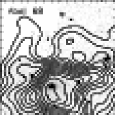
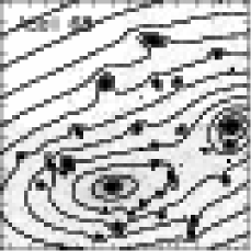
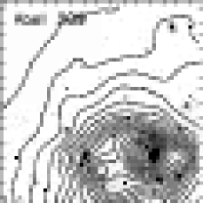
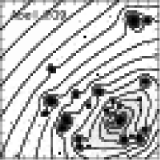
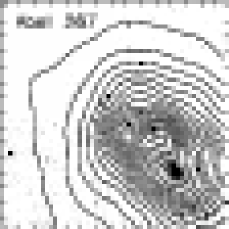
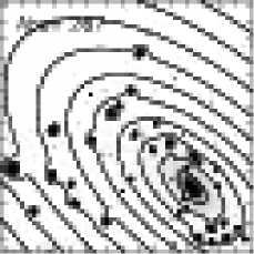
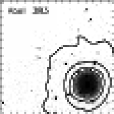
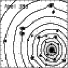
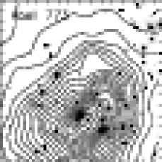
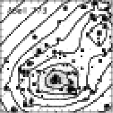
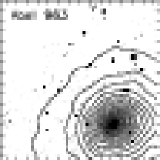
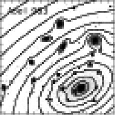
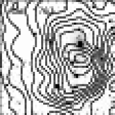
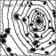
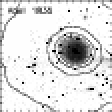
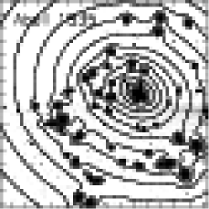
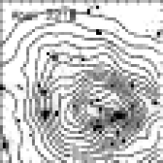
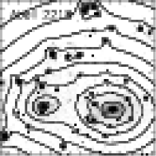
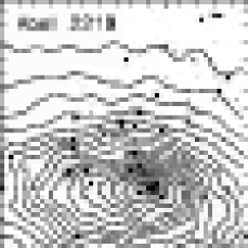
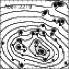
Figure 7: For each cluster in the sample, we show (left) the adaptively smoothed X–ray flux contours and (right) the iso–mass contours calculated from the best–fit lens models. The greyscales are low–resolution renderings of the HST/WFPC2 frame. All three of the clusters classified as relaxed (A 383, A 963 and A 1835; Table 6) have very regular and centrally concentrated X–ray and mass morphologies. The seven unrelaxed clusters all have irregular X–ray morphologies, and four of them (A 68, A 773, A 2218, A 2219) have bi/tri–modal mass morphologies. All contours are equally spaced in the log.

We now compare the cluster mass distributions with the X–ray observations to gain further leverage in diagnosing the maturity of the full sample of 10 clusters.

Iso–mass contours computed from the best–fit lens models and adaptively smoothed X–ray flux contours from the Chandra observations are overplotted on the HST frames in Fig. 7. We also carefully check the pointing accuracy of the Chandra observations using $28^{\prime}{\times}42^{\prime}$ panoramic CFH12k imaging of these cluster fields (Czoske 2002) to confirm that the Chandra astrometry matches the frame defined by the optical data to an rms accuracy of ${\mathrel{\hbox{\hbox to0.0pt{\hbox{\lower 4.0pt\hbox{$\sim$}}\hss}\hbox{$<$}}}}2{\rm kpc}$ at the cluster redshift. We measured the offset between the position of the X–ray peak in each Chandra frame and list ${\mathrel{\Delta r_{\rm peak}}}$, the offset between this position and the center of mass in the mass–maps in Table 6. We compare the mass and X–ray morphologies with the mass and luminosity fractions discussed in §6.1.1. Three of the four high central mass fraction clusters (A 383, A 963, A 1835) appear relaxed at X–ray wavelengths, i.e. circular or mildly elliptical morphology. A 267, is an exception to this picture – its X–ray flux contours are much less regular than the other three systems, and there appears to be a large offset between X–ray and mass centers. The six low central mass fraction clusters also have irregular X–ray morphologies and misalignment between X–ray and mass peaks.

We also list in Table 6 the ratio of the total to annular temperatures (${\mathrel{kT_{X{\rm,tot}}}}/{\mathrel{kT_{X{\rm,ann}}}}$) of each cluster measured in §5 to test for the presence of cool cores. Eight of the clusters, comprising the six with low central mass fractions plus A 267 and A 963 display no evidence of a cool core. The absence of evidence for a cool core in A 267 is unsurprising given the likely dynamical disturbance in the cluster core as indicated by its X–ray morphology. A temperature ratio of unity for A 963 is also consistent with previous work on this cluster, which has traditionally been classified as an “intermediate” cluster (e.g. Allen 1998), i.e. it appears to be quite relaxed, but has not acquired a cool core since (presumed) previous merger activity. This is also consistent with the mild ellipticity in the X–ray isophotes, in contrast to the almost circular isophotes of A 383 and A 1835.

6.1.3 Summary

Table 6 lists all of the diagnostics described in this section. Each diagnostic in isolation offers a slightly different view of the dynamical maturity of each cluster. We combine all of the available information to determine a robust diagnosis of each cluster’s maturity, and to identify the remaining uncertainties. In making the overall classifications listed in Table 6, we define the term “relaxed” to mean that the cluster is dynamically mature in all diagnostics available to us, with the exception that we do not require it to have a cool core. In terms of the diagnostics listed in Table 6, this means that $N_{\rm DM}{=}1$, ${\mathrel{M_{\rm cen}}}/{\mathrel{M_{\rm tot}}}{\geq}0.95$, $L_{K,{\rm BCG}}/L_{K,{\rm tot}}{\mathrel{\hbox{\hbox to0.0pt{\hbox{\lower 4.0pt\hbox{$\sim$}}\hss}\hbox{$>$}}}}0.5$, ${\mathrel{\Delta r_{\rm peak}}}{<}4{\rm kpc}$, and the X–ray morphology is either circular, or mildly elliptical. The unrelaxed clusters do not satisfy one or more of these criteria.

We therefore conclude that 7 out of the 10 clusters in our study, i.e. $70{\pm}20\%$ of X–ray luminous cluster cores at $z{\simeq}0.2$ are dynamically immature (the error bar assumes binomial statistics – Gehrels 1986). Henceforth we classify A 383, A 963 and A 1835 as “relaxed” clusters and A 68, A 209, A 267, A 773, A 1763, A 2218 and A 2219 as “unrelaxed” clusters (Table 6).

6.2 Cluster Scaling Relations

We now investigate the scaling relations between cluster mass, temperature and X–ray luminosity, focusing on the normalization of and scatter around the relations and the impact of the dynamical immaturity of 70% of the sample identified in §6.1.

6.2.1 Mass Versus X–ray Luminosity

The sample is selected on X–ray luminosity (§2), we therefore begin with the mass–luminosity relation. First, we explore whether we can improve on the precision of the RASS–based X–ray luminosities (Table 1) using the Chandra data. One of the largest uncertainties in the luminosities quoted in Table 1 is that ROSAT’s large PSF limited the efficiency with which point–sources could be excised from the cluster data. The sub–arcsecond PSF of the Chandra data overcome this problem, however we find that the corrections for point–sources are modest and comparable with the extrapolation uncertainties that arise from Chandra’s field of view which is too small to embrace all of the extended emission from clusters at $z{=}0.2$. The Chandra–based luminosities are therefore no more precise than the ROSAT luminosities at this redshift. We therefore adopt the X–ray luminosities upon which the sample was selected (Table 1).

We plot ${\mathrel{M_{\rm tot}}}$ versus X–ray luminosity in Fig. 8. Despite selecting very X–ray luminous clusters for this study ($L_{X}{\geq}8{\times}10^{44}\mathrel{\rm erg\,s^{-1}}$, 0.1–2.4 keV), these data span sufficient dynamic range in principal to constrain both the slope and normalization of the mass–luminosity relation (c.f. Finoguenov et al. 2001). We parametrize the mass–luminosity relation as follows:

$$({\mathrel{L_{X}}}/10^{44}{\rm erg\,s^{-1}}){=}A({\mathrel{M_{\rm tot}}}/10^{14}{\mathrel{\rm M_{\odot}}})^{1/\alpha}$$ (1)

and try to solve for $A$ and $\alpha$ following Akritas & Bershady (1996) to account for errors in both variables and unknown intrinsic scatter. Unsurprisingly, given the large scatter that is immediately obvious upon visual inspection of Fig. 8, this exercise fails. We therefore fix the slope parameter and simply measure the normalization, $A$. This is done by computing the mean mass and luminosity, and then solving $\log A{=}\langle\log(L_{X})\rangle{-}\langle\log(M_{\rm tot})\rangle/{\alpha}$. Uncertainties in both mass and luminosity are included in the calculation by repeating it $10^{4}$ times, on each occasion drawing values of $M_{\rm tot}$ and $L_{X}$ randomly from the distributions defined by the error bars on X–ray luminosity and mass listed in Tables 1 and 6 respectively. Simple gravitational collapse models predict that ${\alpha}{=}0.75$ (Kaiser 1986), we therefore initially measure the normalization using this value for the slope, and also compute the intrinsic scatter around this model. These calculations are performed for the whole sample of ten clusters and the relaxed and unrelaxed sub–samples, and the results listed in Table 7. Based on these calculations, there is no evidence for segregation between relaxed and unrelaxed clusters in the mass–luminosity plane, and the scatter is $\sigma_{\rm M}{\simeq}0.4$.

We repeat these calculations using an empirical determination of the slope: ${\alpha}{=}0.76^{+0.16}_{-0.13}$ (Allen et al. 2003), drawing randomly from the error distribution on $\alpha$ in the same manner as described above for the mass and luminosity data. This has the effect of broadening the uncertainties on the normalizations listed in Table 7, but does not change the overall conclusion.

6.2.2 Mass Versus Temperature

Table 7: Scaling Relations – Normalizations and Scatters

Sample	Slopea	Normalization	Scatter
Mass–luminosity: $L{=}A\,M^{1/\alpha}$
All	$\alpha{=}0.75$	$A{=}2.64{\pm}0.36$	$\sigma_{M}{=}0.41$
Relaxed		$A{=}2.63{\pm}0.36$	$\sigma_{M}{=}0.30$
Unrelaxed		$A{=}2.65{\pm}0.50$	$\sigma_{M}{=}0.45$
All	$\alpha{=}0.76^{+0.18}_{-0.13}$	$A{=}2.53{\pm}1.74$	$\sigma_{M}{=}0.41$
Relaxed		$A{=}2.50{\pm}2.05$	$\sigma_{M}{=}0.30$
Unrelaxed		$A{=}2.54{\pm}1.68$	$\sigma_{M}{=}0.45$
Mass–temperature: $kT{=}B\,M^{1/\beta}$
All	$\beta{=}1.5$	$B{=}3.59{\pm}0.24$	$\sigma_{T}{=}0.42$
Relaxed		$B{=}2.76{\pm}0.20$	$\sigma_{T}{=}0.29$
Unrelaxed		$B{=}4.01{\pm}0.36$	$\sigma_{T}{=}0.43$
All	$\beta{=}1.58^{+0.06}_{-0.07}$	$B{=}3.72{\pm}0.30$	$\sigma_{T}{=}0.41$
Relaxed		$B{=}2.88{\pm}0.26$	$\sigma_{T}{=}0.29$
Unrelaxed		$B{=}4.15{\pm}0.41$	$\sigma_{T}{=}0.42$
Luminosity–temperature: $kT{=}C\,L^{1/\gamma}$
All	$\gamma{=}2$	$C{=}2.21{\pm}0.09$	$\sigma_{T}{=}0.33$
Relaxed		$C{=}1.70{\pm}0.07$	$\sigma_{T}{=}0.24$
Unrelaxed		$C{=}2.46{\pm}0.14$	$\sigma_{T}{=}0.30$
All	$\gamma{=}2.09^{+0.29}_{-0.29}$	$C{=}2.22{\pm}0.71$	$\sigma_{T}{=}0.33$
Relaxed		$C{=}1.71{\pm}0.60$	$\sigma_{T}{=}0.24$
Unrelaxed		$C{=}2.48{\pm}0.76$	$\sigma_{T}{=}0.30$

a For each scaling relation, the first slope parameter listed is based on the self–similar collapse (e.g. Kaiser 1986). The second value in each case is taken from recent empirical measurements: Allen et al. 2003; Finoguenov et al. 2001; Markevitch 1998.

     

Figure 8: Mass–luminosity (left), mass–temperature (center) and luminosity–temperature (right) relations for our sample of ten clusters. The relaxed/unrelaxed clusters are shown by the circular/square symbols as explained in the legend. The solid and dashed lines show the best–fit relations normalized by the relaxed and unrelaxed clusters respectively; see §6.2 and Table 7 for further information. The error bars on each line show the uncertainty on the normalization of each relation. In summary, these relations show that the large scatter detected in the mass–luminosity plane appears to be symmetric; in both the mass–temperature and luminosity–temperature planes, the scatter appears to be asymmetric, with the unrelaxed clusters being on average hotter than the relaxed clusters. This segregation is statistically insignificant in the luminosity–temperature plane, and significant at the 2–3$\sigma$ level in the mass–temperature plane.

We plot ${\mathrel{M_{\rm tot}}}$ versus ${\mathrel{kT_{X{\rm,ann}}}}$ in Fig. 8, and parametrize the relation as:

$$({\mathrel{kT_{X{\rm,ann}}}}/1\,{\rm keV}){=}B({\mathrel{M_{\rm tot}}}/10^{14}{\mathrel{\rm M_{\odot}}})^{1/\beta}$$ (2)

Note that we consider $\mathrel{kT_{X{\rm,ann}}}$, and not $\mathrel{kT_{X{\rm,tot}}}$; the results described here are therefore robust to the presence of cool cores in relaxed clusters.

We adopt the theoretically predicted slope: ${\beta}{=}1.5$, which is consistent with observations for the most massive clusters (e.g. Finoguenov et al. 2001; Allen et al. 2001). Following the procedures described above, we measure the normalization and scatter, and list the results in Table 7. Two significant results emerge from this exercise. First, the unrelaxed clusters are on average $40\%$ hotter than the relaxed clusters at 3–${\sigma}$ significance, and second the scatter about the mass–temperature relation for all clusters is ${\sigma_{T}}{\simeq}0.4$. The statistical significance of the temperature off–set is reduced to 2.5–${\sigma}$ if an empirically measured value of ${\beta}$ is used in place of the theoretical value (e.g. ${\beta}{=}1.58^{+0.06}_{-0.07}$ – Finoguenov et al. 2001).

6.2.3 X–ray Luminosity Versus Temperature

Finally, we parametrize the luminosity–temperature relation as:

$$({\mathrel{kT_{X{\rm,ann}}}}/1\,{\rm keV}){=}C({\mathrel{L_{X}}}/10^{44}{\rm erg\,s^{-1}})^{1/\gamma}$$ (3)

and repeat the analysis described above. Adopting the theoretical value of ${\gamma}{=}2$, the measured values of $C$ (Table 7) indicate that unrelaxed clusters are $30\%$ hotter than relaxed clusters, at 2.4–$\sigma$ significance, i.e. less significance than in the mass–temperature plane. However, adopting an empirical measurement of ${\gamma}$ in the fit (${\gamma}{=}2.09{\pm}0.29$ – Markevitch 1998) eliminates the statistical significance in this difference. Nevertheless, this hint of structural segregation in the luminosity–temperature plane (see also Fig. 6) is significant for two reasons. First, it provides a lensing–independent cross–check on the results in the mass–temperature plane, in that both luminosity and temperature measurements are independent of the lens modelling upon which the cluster mass measurements are based. Second, it is consistent with previous detections of structural segregation in the luminosity–temperature plane (e.g. Fabian et al. 1994).

7 Discussion

This is the first study to combine a detailed, high–resolution strong–lensing analysis of an objectively selected cluster sample with analysis of a high–resolution X–ray spectro–imaging dataset. As such, it affords the first opportunity to combine high–quality optical and X–ray probes of cluster mass, structure and thermodynamics. The results presented in the previous section may be summarized as follows:

• $70{\pm}20\%$ of X–ray luminous cluster cores at $z{=}0.2$ are dynamically immature;

• scaling relations between cluster mass, luminosity and temperature display scatter of ${\sigma}{\sim}0.3$–0.6;

• the normalization of the mass–temperature relation for unrelaxed (dynamically immature) clusters is $40\%$ hotter than for relaxed clusters.

We discuss these results in §7.1 and §7.2, and close by considering the implications of the results for the use of massive clusters as cosmological probes (§7.3).

7.1 Dynamical Immaturity of Cluster Cores

Galaxy clusters grow by accreting DM, gas and galaxies from their surroundings, including the filamentary structure (§1). The observed structure of clusters therefore probes a combination of both the in–fall history and the relaxation processes that govern the timescales on which clusters regain equilibrium following cluster–cluster mergers.

The clusters can be grouped into three categories on the basis of the mass and X–ray flux maps in Fig. 7. The least ambiguous category is the relaxed clusters (A 383, A 963 and A 1835 – see §6.1), all of which display a similar degree of relaxation in both mass and X–ray. The other two categories are sub–divisions of the unrelaxed clusters. First, we consider the four unrelaxed clusters with obviously bi/tri–modal mass distributions (A 68, A 773, A 2218 and A 2219). Whilst the X–ray flux contours of these clusters are both irregular and elongated in the same directions as the mass distributions, there is no obvious evidence of bi–modality in the X–ray flux. On radial scales greater than a few tens of kpc from the center of the cluster BCGs, the mass maps should trace the distribution of DM. The ICM in these clusters therefore appears to be more relaxed than the DM distribution. DM is generally believed to be collisionless (Davis et al. 1985; however see also Spergel & Steinhardt 2000); in contrast, the ICM is baryonic and therefore collisional. The absence of X–ray bi–modality in clusters with mass bi–modality therefore qualitatively supports the collisionless DM hypothesis.

The third category comprises the remaining three unrelaxed clusters (A 209, A 267 and A 1763) for which there is no compelling evidence in the current data for bi/tri–modality in the DM distribution. Nevertheless, several clues as to the true DM distributions are present in the data. For example, the strongly elliptical mass distribution of A 267 may indicate that the matter distribution is more complex than a single elongated DM halo plus cluster galaxy population (Edge et al. 2003). Deep wide–field space–based imaging is needed to explore this possibility, specifically to search for evidence of other mass concentrations using weak gravitational lensing (Kneib et al. 2003). Turning to A 1763, galaxies appear to be falling in to this cluster along a ${\sim}2{\rm Mpc}$ long filament (Vallée & Bridle 1982; Bardeau et al. 2004, in prep.). This cluster may therefore be experiencing a merger in the plane of the sky, which is thus poorly sampled by the small field–of–view of the WFPC2 data used in this study. An alternative interpretation of these three clusters is that sufficient time has elapsed since the presumed merger event for the DM distribution to relax and thus not present a bi/tri–modal structure at the epoch of observation. However, given the strong dynamical disturbance in the X–ray flux maps, we consider this unlikely.

Ultimately cross–correlation of mass and X–ray maps of these and similarly selected samples of clusters at higher redshifts will help to constrain the relevant relaxation timescales and processes. Critical next steps towards that goal are to obtain wider–field space–based imaging to overcome uncertainties arising from the current tiny pencil–beam WFPC2 observations of the cluster cores, plus enlargement of the sample to overcome the small number statistics of comparing sub–samples of ${\sim}3$ systems. Uniformly deep X–ray data would also enable tight constraints on the temperature structure of the unrelaxed clusters to be achieved. Such temperature maps would help to more clearly delineate the structure of the ICM in the unrelaxed clusters.

From a theoretical perspective, numerical simulations suggest that both gas dynamics and substructure in the DM distribution may persist for as long as ${\sim}5\,{\rm Gyr}$ following a merger event (Schindler & Müller 1993; Nakamura, Hattori & Mineshige 1995; Roettiger, Loken & Burns 1997; Tormen, Diaferio & Syer 1998; de Lucia et al. 2004). This suggests that despite the expected differences between the physics of the ICM and the DM, the relaxation timescales for these two matter components may be comparable. The differences in cluster X–ray and mass morphologies noted above imply that the X–ray and mass morphological evolution of clusters may follow different evolutionary paths, even if the overall relaxation timescales are indeed comparable. This idea is supported by the numerical simulations of Ricker & Sarazin (2001), who found that oscillations in the gravitational potential of a merging cluster (due to the dominant collisionless DM) sustain turbulence and thus non–relaxation of the ICM on timescales comparable with that required for the DM to achieve equilibrium.

7.2 Cluster Scaling Relations

Numerous observational and theoretical studies of cluster scaling relationships have addressed the slope, normalization and intrinsic scatter of these relations. Structural segregation in the scaling relation planes has also been discussed in the context of cooling–flow and non–cooling–flow clusters in the luminosity–temperature plane (Fabian et al. 1994; Markevitch 1998; Allen & Fabian 1998; Arnaud & Evrard 1999). Adding gravitational lensing as a direct and clean probe of cluster mass to scaling relation studies parallels the importance of adding this diagnostic into the structural studies discussed above. Lensing–based mass estimates have been used to supplement X–ray cluster studies (e.g. Allen et al. 2003), however these studies have relied on weak–lensing data without an absolute mass normalization from strong–lensing constraints. The resulting large error bars therefore significantly degrade the advantage of using lensing as a probe of cluster mass. Smail et al. (1997) attempted to include lensing in cluster scaling relation studies, using the weak–shear signal of optically selected clusters as a surrogate for mass to construct a shear–$L_{X}$ relation. Hjorth et al. (1998) went a step further, using weak–lensing mass estimates to estimate the mass of eight clusters, and thus construct the first lensing–based mass–temperature relation. However, as these authors point out, their use of weak–lensing and heterogeneous selection function undermines the precision of their work.

The important advantage of our study is that the lensing–based mass measurements are based on detailed strong–lensing mass models, the normalization of which are locked down by spectroscopically confirmed multiple–image systems and cross–calibration between strong–lensing and weak–lensing constrained clusters. Combining the lensing results with high quality X–ray spectro–imaging with Chandra places us in a hitherto unique position to explore the mass–temperature plane. We therefore concentrate our discussion of cluster scaling relations in this area. It is also important to note that the mass information extracted from the lensing mass maps is two–dimensional. In contrast, the information extracted from theoretical simulations is three–dimensional. Reliable calibrations between 2– and 3–dimensional cluster masses have not yet been achieved. We therefore concentrate on discussing the scatter in the mass–temperature plane and the related issue of structural segregation, i.e. the relative normalization of relaxed and unrelaxed clusters.

7.2.1 Scatter

Evrard, Metzler & Navarro (1996) predicted that solely a broad–beam measurement of the temperature of ICM in an individual cluster can be used to measure cluster masses to an rms precision of ${\sim}10$–20%. This is in stark contrast to the ${\sigma}_{M}{\simeq}0.6$ scatter in mass that we detect in §6.2. An important clue as to the origin of this difference is that the observational scatter appears to be dominated by the unrelaxed clusters (see Table 7). However several other factors may also contribute to both the size of the observed scatter and the apparent discrepancy between observation and theory.

We first consider the issue of aperture size. The observational mass measurements sample just the central $R{\leq}500{\rm kpc}$ of each cluster; this aperture matches approximately the radius at which the cluster density is $2500{\times}$ the critical density, i.e. $\delta_{c}{=}2500$ (Smith et al. 2003). The scatter may therefore be dominated by systematics relevant only to the very central regions of the clusters. We use the ground–based weak–lensing analysis of the same clusters by Bardeau et al. (2004, in prep.) to make a preliminary estimate of how the scatter may reduce if the current analysis were extended to larger radii ($\delta_{c}{\simeq}500$). The uncertainties on Bardeau et al.’s results are largely due to the poor spatial resolution of ground–based data relative to our HST data. However comparison of the two datasets suggests that one–third of the scatter may be due to the small aperture size employed in this study. This variation in scatter as a function of overdensity is consistent with recent observational results in the X–ray pass–band (e.g. Ettori, De Grandi & Molendi 2002). Therefore, after taking account of aperture size, the scatter remains a factor of ${\sim}3$ larger than the simulations.

A further potentially important issue is that of selection effects. Ricker & Sarazin’s (2001; see also Ritchie & Thomas 2002) simulations suggest that cluster–cluster mergers boost cluster X–ray luminosities on timescales of a few Gyrs. This may lead our X–ray luminosity selected sample to be biased toward merging systems. However the most luminous cluster in the sample is A 1835, a canonical relaxed cluster with a cool core, indeed a central excess of X–ray flux is a signature of the most relaxed clusters. Overall, the details of cluster selection are a complicated subject, however there is no strong evidence that the sample is biased toward unrelaxed systems. Nevertheless, a careful like–for–like comparison between synthetic and observational cluster selection functions is an important outstanding task.

In summary, we find a factor of 3 more scatter in the mass–temperature relation than predicted. Further work is required to ensure that measurement methods applied to synthetic and observed datasets are well matched, and to extend the space–based lensing results to wider fields–of–view. However, even after this work has been completed, the disagreement between observation and theory may persist, which would be a signature of missing physics in the theoretical descriptions of cluster assembly and relaxation.

7.2.2 Structural Segregation

In §6.2 we identified that unrelaxed clusters are 40% hotter than relaxed clusters at 2.5–${\sigma}$ significance. Clearly, the aperture size issue noted above also impacts on this result, and wider–field space–based weak–lensing observations of a statistically complete sample are critical to a thorough investigation of this uncertainty. Nevertheless, the comparison with Bardeau et al.’s (2004, in prep.) ground–based weak–lensing results provides important reassurance that a substantial fraction of the 40% temperature offset is a genuine physical effect.

Indeed, recent observational and theoretical work supports the idea that unrelaxed clusters are hotter than relaxed systems. Using spatially resolved spectroscopy with BeppoSAX, Ettori, De Grandi & Molendi (2002) identified the normalization of the mass–temperature relation of “non–cooling flow” clusters to be hotter than that of “cooling flow” clusters, however the large uncertainties limited the statistical significance of this result. On the theoretical side, Ricker & Sarazin’s (2001) simulations of cluster–cluster mergers indicate that merger–induced boosts of up to a factor of ten (the amplitude of the boost depends on the mass ratio between the merging clusters and the impact parameter of the collision) in temperature can occur on short timescales (${\mathrel{\hbox{\hbox to0.0pt{\hbox{\lower 4.0pt\hbox{$\sim$}}\hss}\hbox{$<$}}}}1{\rm Gyr}$) due to shock–heating of the gas in a major merger. This relatively brief luminosity boost suggests that not many clusters in our sample should have temperatures ${\mathrel{\hbox{\hbox to0.0pt{\hbox{\lower 4.0pt\hbox{$\sim$}}\hss}\hbox{$>$}}}}3{\times}$ higher than the mean relation. This is indeed the case, with A 2219 being the possible sole example of a cluster currently experiencing a temperature boost of this magnitude. This cluster has previously been identified as having recently experienced a core–penetrating merger (e.g. Smail et al. 1995; Giovannini, Tordi & Feretti 1999)

Despite the short–lived extreme temperature boosts, merger remnants appear to asymptote to temperatures ${\sim}10$–40% higher than the pre–merger configuration, the precise long–term boost again depending on the mass ratio and impact geometry. Assuming that elimination of aperture size and related issues (§7.2.1) reduces the temperature offset between relaxed and unrelaxed clusters to ${\sim}20$–30%, these theoretical results support the idea that the cluster mergers are responsible for the structural segregation of clusters in the mass–temperature plane.

If empirically clusters are either relaxed hosts of cool cores, or unrelaxed (i.e. merging or merger remnant) systems without cool cores, then merger–boosts may be sufficient to explain the structural segregation. However deep integrations with Chandra and XMM–Newton indicate that the picture may not be so clear–cut. For example some cool core clusters appear to be undergoing merger activity (e.g. Perseus – Churazov, et al. 2003), and some dynamically relaxed clusters do not host a cool core (e.g. A 963 in this work). The significance of merging cool core clusters and relaxed non–cool core clusters for the merger–boost interpretation of structural segregation in the mass–temperature plane is unclear at this time. For example the mass ratio of the Perseus merger may be so large (i.e. the mass of the in–falling system so small relative to Perseus) as to not be relevant to the current discussion. However it does suggest that alternative mechanisms such as cluster–to–cluster variations in the level of initial pre–heating may be an additional complication when interpreting the demographics of relaxed/unrelaxed and cool core/non–cool core clusters (Babul, McCarthy & Poole, 2003).

7.3 Implications for Cluster Cosmology

Massive galaxy clusters are one of a number of complementary probes of cosmological parameters. For example, many studies have used empirical determinations of cluster scaling relations to convert the observed X–ray luminosity and/or temperature functions into mass functions. The most massive clusters are rare objects, and thus the constraints on the high–mass end of the mass function inferred from such experiments enables constraints on a combination of ${\Omega}_{\rm M}$ and ${\sigma}_{8}$ in principal to be achieved. Recent cluster–based estimates of ${\sigma}_{8}$ have yielded discrepant results, with most estimates of ${\sigma}_{8}$ falling in the range ${\sim}$0.6–1 (e.g. Eke et al. 1996; Nevalainen, Markevitch & Forman 2000; Allen, Schmidt & Fabian 2001; Borgani et al. 2001; Pierpaoli, Scott & White 2001; Reiprich & Böhringer 2002; Viana et al. 2002). The critical step in these experiments is the conversion from observable (i.e. X–ray luminosity or temperature) to mass. Our results suggest that care must be taken to incorporate sufficient scatter in the observable–mass relationship. The asymmetric scatter of the mass–temperature relationship arising from structural segregation of clusters in this plane implies that such issues may be most acute when converting from cluster temperature to mass, especially if the cluster selection function is poorly characterized. Indeed, in a companion to this article, Smith et al. (2003) showed that incomplete understanding of the cluster selection function can cause ${\sim}20\%$ systematic uncertainties in ${\sigma}_{8}$, favouring values to the lower end of the range found in other recent works.

In a similar vein, we note that our results will likely impinge on cosmological results derived from SZE surveys (see Carlstrom, Holder & Reese 2002 for a recent review). Again, the key issue is the precision to which the observable–mass relationship is known; in this case the observable is the temperature of the ICM, as derived from the SZE signal. The issues for SZE surveys may be aggravated because the goal of measuring the dark energy equation–of–state parameter $w$, relies at least in part on measuring the evolution of the cluster population between two redshifts straddling the epoch at which the dark energy is thought to take over as the dominant factor in the expansion of the universe. This is in contrast to measuring a combination of ${\sigma}_{8}$ and ${\Omega}_{\rm M}$ from studies of local clusters, i.e. just one redshift slice. Further detailed wide–field investigations of massive clusters at both low ($z{=}0.2$) and higher ($z{\mathrel{\hbox{\hbox to0.0pt{\hbox{\lower 4.0pt\hbox{$\sim$}}\hss}\hbox{$>$}}}}0.6$) redshifts are therefore needed to quantify robustly the evolution of the dynamical maturity of clusters and the impact of that on cluster scaling relations. We suggest that, in the light of major imminent SZE cluster surveys, this is an urgent exercise.

8 Summary and Conclusions

We have undertaken a comprehensive study of the distribution of mass in ten X–ray luminous ($L_{X}{\geq}8{\times}10^{44}{\rm erg\,s^{-1}}$[0.1–2.4 keV]) galaxy clusters at $z{=}0.21{\pm}0.04$. The cornerstone of our analysis is a suite of detailed gravitational lens models that describe the distribution of total mass in the cluster cores. These models are constrained by the gravitational lensing signal detected in high–resolution HST/WFPC2 imaging of the clusters, including numerous multiply–imaged and weakly–sheared background galaxies. Analysis of archival Chandra observations complements the lensing analysis and enables us to relate the total mass and structure of the clusters to the thermodynamics of the intra–cluster medium. We re–cap the key results.

• Five of the ten clusters contain spectroscopically confirmed strong gravitational lensing, i.e. multiply–imaged background galaxies. These five clusters comprise: A 68 (Smith et al. 2002b; §3.2), A 383 (Smith et al. 2001; Sand et al. 2004), A 963 (Ellis et al. 1991), A 2218 (Pelló et al. 1992; Ebbels et al. 1998; Ellis et al. 2002) and A 2219 (§3.2).

• Of the remaining five clusters, two contain relatively unambiguous examples of strong lensing for which spectroscopic redshifts are not yet available (A 267 and A 1835). The other three clusters, A 209, A 773 and A 1763 do not contain any obviously multiply–imaged galaxies, however the optical richness and massive nature of A 773 imply that this cluster may well contain strong lensing that has yet to be uncovered.

• Based on our search for strong–lensing in these clusters down to a surface brightness limit of $\mu_{702}{\simeq}25$ mag arcsec^-2, we therefore put a firm lower limit on the fraction of the cluster sample that have a central projected mass density in excess of the critical density required for gravitational lensing of $50\%$. Including A 267 and A 1835 increases this limit to $70\%$.

• We use the strong– and weak–lensing signals to constrain parametrized models of the cluster potential wells, and from these models compute maps of the total projected mass in the cluster cores. Spatial analysis of these maps reveals that four of the clusters form a homogeneous sub–sample with very high central mass fractions (${\mathrel{M_{\rm cen}}}/{\mathrel{M_{\rm tot}}}{>}0.95$). The remaining six are strongly heterogeneous, with central mass fractions in the range $0.4{\leq}{\mathrel{M_{\rm cen}}}/{\mathrel{M_{\rm tot}}}{\leq}0.9$. The central mass fraction of ${\mathrel{M_{\rm cen}}}/{\mathrel{M_{\rm tot}}}{\simeq}0.95$ that divides these two populations corresponds to a $K$–band central luminosity fraction of $L_{\rm K,BCG}/L_{\rm K,tot}{\sim}0.5$.

• All of the six low central mass fraction clusters have an irregular, but not obviously bi/tri–modal X–ray morphology. Four of the six are constrained by the current lensing data to have a bi/tri–modal mass morphology (A 68, A 773, A 2218, A 2219). The other two (A 209 and A 1763) may be merging in the plane of the sky and thus any multi–modality in their mass distributions is not well–sampled by our WFPC2 pencil–beam survey of the cluster cores.

• Three of the four high central mass fraction clusters also have relaxed X–ray morphologies. The remaining cluster (A 267) has a disturbed X–ray morphology, with a ${\sim}90$ kpc offset between its centers of X–ray emission and mass. The distribution of mass in this cluster may therefore be more complex than the single dark matter halo (plus cluster galaxies) that the current data are able to constrain.

• Combining all of the information available to us, we define “relaxed” clusters to be those which appear relaxed in all available diagnostics, with the exception that we do not require a cool core. Quantitatively relaxed clusters therefore have a single cluster–scale DM halo in their lens model ($N_{\rm DM}{=}1$), a high central mass fraction (${\mathrel{M_{\rm cen}}}/{\mathrel{M_{\rm tot}}}{\geq}0.95$) and central $K$–band luminosity fraction ($L_{K,{\rm BCG}}/L_{K,{\rm tot}}{\mathrel{\hbox{\hbox to0.0pt{\hbox{\lower 4.0pt\hbox{$\sim$}}\hss}\hbox{$>$}}}}0.5$), no evidence for an offset between the X–ray emission and the center of mass ${\mathrel{\Delta r_{\rm peak}}}{<}4{\rm kpc}$) and the X–ray morphology is either circular, or mildly elliptical. The unrelaxed clusters do not meet at least one of these criteria.

• Applying these criteria to the cluster sample, we conclude that seven of the ten clusters are dynamically immature, i.e. unrelaxed (A 68, A 209, A 267, A 773, A 1763, A 2218, A 2219) and three are relaxed (A 383, A 963, A 1835); thus, formally $70{\pm}20\%$ of X–ray luminous cluster cores at $z{=}0.2$ are unrelaxed.

• We detect a factor of three more scatter in the mass–temperature plane than predicted by Evrard, Metzler & Navarro (1996), implying that great care should be exercised when using such relations to convert cluster temperature functions to mass functions in pursuit of cosmological parameters. We also consider a number of key uncertainties that may artificially inflate our estimate of the scatter. This exercise suggests that approximately one third of the scatter detected in this study may be due to issues related to the small field–of–view of our WFPC2 observations.

• The scatter in the mass–temperature plane is asymmetric, presenting evidence of structural segregation. The normalization of the mass–temperature relation for unrelaxed (dynamically immature) clusters is $40\%$ hotter than for relaxed clusters at 2.5–${\sigma}$ significance. This result is consistent with recent simulations of cluster–cluster mergers (Ricker & Sarazin 2001; Randall, Sarazin & Ricker 2002), implying that merger induced temperature boosts may be the dominant factor behind the hotter normalization of unrelaxed systems.

In summary, this study is the first of its kind, exploiting detailed strong–lensing constraints on the distribution of mass in X–ray luminous cluster cores, complemented by X–ray spectro–imaging with Chandra. The high frequency of dynamical immaturity, coupled with the structural segregation of the clusters in the mass–temperature plane have profound implications for our understanding of how clusters form and evolve. Perhaps of greatest importance at this time is the implications of these results for using clusters to constrain the cosmological parameters, ${\Omega}_{M}$, ${\sigma}_{8}$ and the dark energy equation–of–state parameter $w$. In a companion paper we demonstrate that inadequate knowledge of the cluster selection function can lead to $20\%$ systematic errors in cluster–based measurements of ${\sigma}_{8}$. Turning to $w$, forthcoming Sunyaev–Zeldovich Effect experiments designed to detect and measure the mass of clusters out to high redshifts, using mass–temperature scaling relations may be compromised by unidentified and/or poorly calibrated astrophysical systematic uncertainties (see also Majumdar & Mohr 2003).

Our future program will build on these results in three ways. First, we aim to overcome the principal uncertainties in the current work: small number statistics and tiny field–of–view. Wide–field space–based imaging of a statistically complete sample of clusters would be essential to achieve this goal. Second, detailed comparison of selection effects and measurement techniques between theoretical and observational studies will enable more detailed and rigorous comparison between observational and synthetic datasets. Finally, we are gathering HST/ACS imaging of an identically selected sample of clusters at $z{\simeq}0.55$ drawn from the MACS sample (Ebeling et al. 2001b). We will combine these data with observations in the X–ray pass–band and compare the results to those found here. The ${\sim}3$ Gyr difference in look–back–time between $z{=}0.2$ and $z{=}0.55$ will enable us to search for evolutionary trends in the most massive clusters.

References

• Abell G.O., Corwin H.G. Jr., Olowin R.P., 1989, ApJS, 70, 1

• Adami C., Ulmer M.P., Durret F., Nichol R.C., Mazure A., Holden B.P., Romer A.K., Savine C., 2000, A&A, 353, 930

• Akritas M.G., Bershady M.A., 1996, ApJ, 470, 706

• Allen C.W., 1973, Astrophysical Quantities, 3rd edn. Athlone Press, London

• Allen S.W., Fabian A.C., Kneib J.-P., 1996, MNRAS, 279, 615

• Allen S.W., 1998, MNRAS, 296, 392

• Allen S.W., Fabian A.C., 1998, MNRAS, 297, 57

• Allen S.W., Schmidt R.W., Fabian A.C., 2001, MNRAS, 328, L37

• Allen S.W., Schmidt R.W., Fabian A.C., Ebeling H., 2003, MNRAS, 342, 287

• Arnaud M., Evrard A.E., 1999, MNRAS, 309, 631

• Babul A., McCarthy I.G., Poole G.B., 2003, to appear in the proceedings of the “Multiwavelength Cosmology” Conference held in Mykonos, Greece, June 2003, ed. M. Plionis (Kluwer), astro–ph/0309543

• Balogh M.L., Smail I., Bower R.G., Ziegler B.L., Smith G.P., Davies R.L., Gaztelu A., Kneib J.-P., Ebeling H., 2002, ApJ, 566, 123

• Bertin E., Arnouts S., 1996, A&A, 117, 393

• Bézecourt J., Hoekstra H., Gray M.E., AbdelSalaam H.M., Kuijken K., Ellis R.S., 2000, A&A, submitted, astro–ph/0001513

• Bond J.R., Kofman L., Pogosyan D., 1996, Nature, 380, 603

• Borgani S., et al., 2001, ApJ, 561, 13

• Brainerd T.G., Blandford R.D., Smail I., 1996, ApJ, 446, 623

• Buote, D.A., Tsai, J.C., 1996 ApJ, 458, 27

• Carlstrom J.E., Holder G.P., Reese E.D., 2002, ARA&A, 40, 643

• Casertano S., Wiggs M., 2001, “An Improved Goemetric Solution for WFPC2”, ISR WFPC2-2001-10

• Churazov E., Forman W., Jones C., Böhringer H., ApJ, 590, 225

• Cole S., Norberg P., Baugh C.M., Frenk C.S., & the 2dFGRS team, 2001, MNRAS, 326, 255

• Crawford C.S., Allen S.W., Ebeling H., Edge A.C., Fabian A.C., 1999, MNRAS, 306, 857

• Czoske O., Kneib J.-P., Soucail G., Bridges T.J., Mellier Y., Cuillandre J.-C., 2001, A&A, 372, 391

• Czoske O., Moore B., Kneib J.-P., Soucail G., 2002, A&A, 386, 31

• Czoske O., 2002, PhD Thesis, Observatoire Midi-Pyrénées, Université Paul Sabatier, Toulouse, France

• Davis M., Efstathiou G., Frenk C.S., White S.D.M., 1985, ApJ, 292, 371

• De Grandi, S. et al., 1999, ApJ, 514, 148

• De Lapparent V., Geller M.J., Huchra J.P., 1986, ApJ, 302, 1

• De Lucia G., et al., 2004, MNRAS, 348, 333

• De Propris R., et al., 2003, ApJ, 598, 20

• Dickey, J.M., Lockman, F.J., 1990, ARA&A, 28, 215

• Dressler A., Shectman S.A., 1988, AJ, 95, 985

• Ebbels T.M.D., Ellis R.S., Kneib J.-P., Le Borgne J.-F., Pelló R., Smail I., Sanahuja B., 1998, MNRAS, 295, 75

• Ebbels T.M.D., 1998, PhD Thesis, University of Cambridge, UK

• Ebeling H., et al., 1996, MNRAS, 281, 799

• Ebeling H., et al., 1998, MNRAS, 301, 881

• Ebeling H., Edge, A.C., Henry J.P., 2000, in Large Scale Structure in the X–ray Universe, Proceedings of the 20-22 September 1999 Workshop, Santorini, Greece, eds. Plionis, M., Georgantopoulos, I., Atlantisciences, Paris, France, p.39

• Ebeling H., Edge A.C., Henry J.P., 2001, ApJ, 553, 668

• Edge A.C., Stewart G.C., Fabian A.C., Arnaud K.A., 1990, MNRAS, 245, 559

• Edge A.C., Smith G.P., Sand D.J., Treu T., Ebeling H., Allen S.W., van Dokkum P.G., 2003, ApJ, 599, L69

• Eke, V.R., Cole, S., Frenk, C.S., 1996, MNRAS, 282, 263

• Ellis R.S., Allington-Smith J., Smail I., 1991, MNRAS, 249, 184

• Ellis R.S., Santos M.R., Kneib J.-P., Kuijken K., 2001, ApJ, 560, L119

• Ettori S., De Grandi S., Molendi S., 2002, A&A, 391, 841

• Evrard A.E., Mohr J.J., Fabricant D.G., Geller M.J., 1993, ApJ, 419, L9

• Evrard A.E., Metzler C.A., Navarro J.F., 1996, ApJ, 469, 494

• Evrard A.E., et al., 2002, ApJ, 573, 7

• Fabian A.C., Crawford C.S., Edge A.C., Mushotzky R.F., 1994, MNRAS, 267, 779

• Fernández-Soto A., Lanzetta K.M., Yahil A., 1999, ApJ, 513, 34

• Finoguenov A., Reiprich T.H., Böhringer H., 2001, A&A, 368, 749

• Fruchter, A.S., Hook, R.N., 1997, in Applications of Digital Image Processing, Proc. SPIE, 3164, ed. Tescher, A., p120

• Geller M.J., Beers T.C., 1982, PASP, 94, 421

• Gehrels N., 1986, ApJ, 303, 336

• Gilmozzi R., Ewald S., Kinney E., 1995, “The Geometric Distortion Correction for the WFPC Cameras”, ISR WFPC2-95-02

• Gioia I.M., et al., 1990, ApJ, 356, L35

• Giovannini G., Tordi M., Feretti L., 1999, NewA, 4, 141

• Goto T., Okamura S., McKay T.A., Annis J., Bahcall N.A., Bernardi M., Brinkmann J., Gomez P.L., Hansen S., Kim R.S.J., Sekiguchi M., Sheth R., 2002, PASJ, accepted, astro-ph/0205413

• Gunn J.E., Gott J.R.III, 1972, ApJ, 176, 1

• Hjorth J., Oukbir J., van Kampen E., 1998, MNRAS, 298, L1

• Hoekstra H., Franx M., Kuijken K., Squires G., 1998, ApJ, 504, 636

• Hogg D.W., Pahre M.A., McCarthy J.K., Cohen J.G., Blandford R., Smail I., Soifer B.T., 1997, MNRAS, 288, 404

• Holtzman, J.A., Burrows, C.J., Casertano, S., Hester, J.J., Trauger, J.T., Watson, A.M., Worthey, G., 1995, PASP, 107, 1065

• Johnson H.L., 1966, ARA&A, 4, 193

• Jones C., Forman W., 1984, ApJ, 276, 38

• Kaiser N., 1986, MNRAS, 222,323

• Kashikawa N., et al., 2002, PASJ, 54, 819

• Kassiola A., Kovner I., 1993, ApJ, 417, 450

• King C.R., Ellis R.S., 1985, ApJ, 288, 456

• Kneib J.-P., 1993, PhD Thesis, Université Paul Sabatier, Toulouse, France

• Kneib J.-P., Mellier Y., Fort B., Mathez G., 1993, A&A, 273, 367

• Kneib J.-P., Mellier, Y., Fort, B., Soucail, G., Longaretti, P.Y., 1994, A&A, 286, 701

• Kneib J.-P., Mellier Y., Pelló R., Miralda-Escudé J., Le Borgne J.-F., Böhringer H., Picat J.-P., 1995, A&A, 303, 27

• Kneib, J.-P., Ellis, R.S., Smail, I., Couch, W.J., Sharples, R.M., 1996, ApJ, 471, 643

• Kneib J.-P., Hudelot P., Ellis R.S., Treu T., Smith G.P., Marshall P., Czoske O., Smail I., Natarajan P., 2003, ApJ, 598, 804

• Luppino G.A., Gioia I.M., Hammer F., Le Fèvre O., Annis J.A., 1999, A&A, 136, 117

• Majumdar S., Mohr J.J., 2003, ApJ, 585, 603

• Mannucci F., Basile F., Cimatti A., Daddi E., Poggianti B.M., Pozzetti L., Vanzi L., 2001, MNRAS, 326, 745

• Markevitch M., 1998, ApJ, 504, 27

• Markevich, M. et al. 2000a, CXC memo (http://asc.harvard.edu/cal “ACIS”, “ACIS Background”)

• Markevitch, M., et al. 2000, ApJ, 541, 542

• Markevitch, M., & Vikhlinin, A. 2001, ApJ, 563, 95

• Markevitch, M., 2002, astro-ph/0205333

• Marty P.B., Kneib J.-P., Sadat R., Bernard J.-P., Czoske O., Ebeling H., Smail I., Smith G.P., 2004, A& A, submitted

• Mazzotta P., Markevitch M., Vikhlinin A., Forman W.R., David L.P., Van Speybroeck L., 2001, ApJ, 555, 205

• Mellier, Y., Fort, B., Kneib J.-P., 1993, ApJ, 407, 33

• Miralda–Escudé J., Babul A., 1995, ApJ, 449, 18

• Miyazaki S., et al., 2002, ApJ, 580, L97

• Nakamura F.E., Hattori M., Mineshige S., 1995, A&A, 302, 6009

• Nevalainen J., Markevitch M., Forman W., 2000, ApJ, 532, 694

• Oke, J.B., et al., 1995, PASP, 107, 375

• Peacock J.A., et al., 2001, Nature, 410, 169

• Peebles P.J.E., 1980, “Large Scale Structure of the Universe”, Princeton University Press, Princeton

• Pelló R., Le Borgne J.-F., Sanahuja B., Mathez G., Fort B., 1992, A&A, 266, 6

• Peres, C.B., Fabian, A.C., Edge, A.C., Allen, S.W., Johnstone, R.M., White, D.A., 1998, MNRAS, 298, 416

• Pierpaoli E., Scott D., White M., 2001, MNRAS, 325, 77

• Randall S.W., Sarazin C.L., Ricker P.M., ApJ, 577, 579

• Reiprich T.H., Böhringer H., 2002, ApJ, 567, 716

• Rhodes J.D., Refregier A., Groth E.J., 2000, ApJ, 536, 79

• Richstone D., Loeb A., Turner E.L., 1992, ApJ, 393, 477

• Ricker P.M., Sarazin, C.L., 2001, ApJ, 561, 621

• Ritchie B.W., Thomas P.A., 2002, MNRAS, 329, 675

• Roettiger, K., Loken C., Burns J.O., 1997, ApJS, 109, 307

• Sand D.J., Treu T., Ellis R.S., 2002, ApJ, 574, L129

• Sand D.J., Treu T., Smith G.P., Ellis R.S., 2004, ApJ, 604, 88

• Schindler S., Mueller E., 1993, A&A, 272, 137

• Schmidt R.W., Allen S.W., Fabian A.C., 2001, MNRAS, 327, 1057

• Schuecker P., Böhringer H., Reiprich T.H., Feretti L., 2001, A& A, 378, 408

• Shectman S.A., et al., 1996, ApJ, 470, 172

• Smail, I., Couch, W.J., Ellis, R.S.,Sharples, R.M., 1995, ApJ, 440, 501

• Smail I., Hogg D.W., Blandford R., Cohen J.G., Edge A.C., Djorgovski S.G., 1995b, MNRAS, 277, 1

• Smail, I., et al., 1996, ApJ, 469, 508

• Smail, I., Ellis, R.S., Dressler, A., Couch, W.J., Oemler, A., Butcher, H., Sharples, R.M., 1997, ApJ, 470, 70

• Smith G.P., Kneib J.-P., Ebeling H., Csozke O., Smail I., 2001, ApJ, 552, 493

• Smith G.P., Smail I., Kneib J.–P., Czoske O., Ebeling H., Edge A.C., Pello R., Ivison R.J., Packham C., Le Borgne J.–F., 2002, MNRAS, 330, 1

• Smith G.P., Smail I., Kneib J.-P., Davis C.J., Takamiya M., Ebeling H., Czoske O., 2002, MNRAS, 333, L16

• Smith G.P., 2002, PhD Thesis, University of Durham, UK, available upon request from gps@astro.caltech.edu

• Smith G.P., Edge A.C., Eke V.R., Nichol R.C., Smail I., Kneib J.-P., 2003, ApJ, 590, L79

• Spergel D.N., Steinhardt P.J., 2000, Phys. Rev., 84, L3760

• Squires G., Neumann D.M., Kaiser N., Arnaud M., Babul A., Böhringer H., Fahlman G., Woods D., 1997, ApJ, 482, 648

• Squires G., Kaiser N., Fahlman G., Babul A., Woods D., 1996, ApJ, 469, 73

• Swinbank A.M., Smith J., Bower R.G., Bunker A., Smail I., Ellis R.S., Smith G.P., Kneib J.-P., Sullivan M., Allington-Smith J.R., 2003, ApJ, 598, 162

• Tormen G., Diaferio A., Syer D., 1998, MNRAS, 229, 728

• Trauger J.T., Vaughan A.H., Evans R.W., Moody D.C., 1995, “Geometry of the WFPC2 Focal Plane”, in Calibrating HST: Post Service Mission, eds. A. Koratkar & C. Leitherer

• Tyson J.A., Kochanski G.P., dell’Antonio I.P., 1998, ApJ, 498, L107

• Vallée J.P., Bridle A.H., 1982, ApJ, 253, 479

• Vettolani G., et al., 1997, A&A, 325, 954

• Viana, P.T.P., Liddle, A.R., 1996, MNRAS, 281, 323

• Viana P.T.P., Nichol R., Liddle A.R., 2002, ApJ, 569, L75

• Vikhlinin, A., Markevitch, M., Murray, S.S. 2001a, ApJ, 551, 160

• West M.J., Bothun G.D., 1990, ApJ, 350, 36

• White D.M., Jones C., Forman W., 1997, MNRAS, 292, 419

• Wittman D., et al., 2003, ApJ, 597, 218

• Wu X., Fang L., 1997, ApJ, 483, 62

• Wu X.; Chiueh T., Fang L., Xue Y., 1998, MNRAS, 301, 861

• Wu X., 2000, MNRAS, 316, 299

• Yoshida N., et al., 2001, MNRAS, 325, 803

• Zehavi I., et al., 2002, ApJ, 571, 172

Appendix A Gravitational Lens Modelling – Method

This appendix describes relevant details of how the lenstool ray–tracing code is used to construct robust models of the distribution of mass in galaxy clusters using both strong– and weak–lensing constraints.

A.1 Mathematical Overview

Consider a single source at $\mathrel{z_{\rm S}}$ that appears to an observer under the action of a gravitational lens at $\mathrel{z_{\rm L}}$ as $N$ distinct images at positions $\vec{u}_{i}\,(1{\leq}i{\leq}N)$. We describe the source with $\nu$ free parameters, $\Pi_{j}\,(1{\leq}j{\leq}\nu)$, for example: the position of the center of the source, the ellipticity, the orientation, the surface brightness. We write the transformation equations in the following form:

$$\Pi_{j}^{S}{=}f_{j}(\Pi_{ji}^{I},\varphi(\vec{u}_{i}))~{}~{}~{}~{}~{}(1{\leq}i{\leq}N)~{}~{}(1{\leq}j{\leq}\nu)$$ (4)

where $f_{j}$ are functions that depend on the parameters that describe the observed images and the gravitational potential of the lens. The source parameters , $\Pi_{j}^{S}$, and the lens potential, $\varphi(\vec{u}_{i})$, are the unknowns in these equations. We use the image parameters , $\Pi_{ji}^{I}$ (i.e. the observables), to constrain both the source parameters and the lens potential. If we are able to recover $\nu$ parameters for each image, then we have $\nu(N{-}1)$ constraints on our lens model. Generalizing this to $n$ sets of multiple images of sources at redshifts $\mathrel{z_{\rm S}}_{i}$, each multiple-image system being characterized by $(\nu_{i},N_{i})$, then the total number of constraints $n_{c}$ is given by:

$$n_{c}{=}\sum_{i}^{n}[\nu_{i}(N_{i}{-}1){-}\epsilon_{i}]$$ (5)

where $\epsilon_{i}{=}0$ if $\mathrel{z_{\rm S}}_{i}$ is known and $\epsilon_{i}{=}1$ if $\mathrel{z_{\rm S}}_{i}$ is not known (Kneib et al. 1993). Strictly, Equation 5 only applies in the idealized case of all multiple-images being resolved, and none of the images being merging pairs. Clearly higher resolution imaging will increase $n_{c}$.

We describe each observed gravitational image with the following parameters: $\Pi^{I}{=}(\vec{u}^{I},S^{I},\vec{\tau}^{I})$, where $\vec{u}^{I}$ is the position of the image, $S^{I}$ is the observed flux and $\vec{\tau}^{I}{=}\tau^{I}e^{2i\theta^{I}}$ is the complex deformation of the image, describing its ellipticity ($\tau$) and orientation ($\theta$). We use these quantities and their counterparts in the source-plane to write down the transformation equations:

$$\begin{array}[]{ll}{\rm Position:}&\vec{u}^{S}{=}\vec{u}^{I}{-}\vec{\nabla}\varphi(\vec{u}^{I})\cr{\rm Flux:}&S^{S}{=}|{\rm det}\,J|S^{I}\cr{\rm Shape:}&{\rm sgn}({\rm det}\,J)\mathrel{\bf{\vec{\tau}}}^{S}{=}\mathrel{\bf{\vec{\tau}}}^{I}{-}\mathrel{\bf{\vec{\tau}}}_{\rm pot}[\delta^{I}{-}\tau^{I}\Re(\mathrel{\vec{g}}^{I}\mathrel{\vec{g}}^{*}_{\rm pot})]\cr\end{array}$$ (6)

where the first equation is simply the lens equation, $J$ is the Jacobian matrix of the lensing transformation, $\delta{=}(1{+}\tau^{2})^{1/2}$, $\mathrel{\vec{g}}{=}\mathrel{\bf{\vec{\gamma}}}/(1{-}\kappa)$, the subscript “pot” denotes quantities applicable to a circular source (see Kneib et al. (1996) and references therein for a detailed derivation of the shape transformation equation), $\Re$ takes the real part of dot-product between $\mathrel{\vec{g}}^{I}$ and $\mathrel{\vec{g}}^{*}_{\rm pot}$, and $\mathrel{\vec{g}}^{*}$ is the complex conjugate of $\mathrel{\vec{g}}$.

A.2 Parametrization of the Lens Plane Mass Distribution

Each mass component is parametrized as a smoothly truncated pseudo-isothermal elliptical mass distribution (PIEMD – Kassiola & Kovner 1993; Kneib et al. 1996). This functional form is physically well motivated (it avoids the central singularity and infinite spatial extent of singular isothermal models) and can describe mass distributions of arbitrarily large ellipticities. Each PIEMD mass component is parametrized by its position ($\mathrel{x_{\rm c}}$, $\mathrel{y_{\rm c}}$), ellipticity ($\epsilon$), orientation ($\theta$), core radius ($\mathrel{r_{\rm core}}$), cut-off radius ($\mathrel{r_{\rm cut}}$) and central velocity dispersion ($\mathrel{\sigma_{\rm o}}$), and the projected mass density, $\Sigma$ is given by:

$$\Sigma(x,y){=}\frac{\mathrel{\sigma_{\rm o}}^{2}}{2G}\,\frac{\mathrel{r_{\rm cut}}}{\mathrel{r_{\rm cut}}{-}\mathrel{r_{\rm core}}}\left(\frac{1}{(\mathrel{r_{\rm core}}^{2}{+}\rho^{2})^{1/2}}{-}\frac{1}{(\mathrel{r_{\rm cut}}^{2}{+}\rho^{2})^{1/2}}\right)$$ (7)

where $\rho^{2}{=}[(x{-}\mathrel{x_{\rm c}})/(1{+}\epsilon)]^{2}{+}[(y{-}\mathrel{y_{\rm c}})/(1{-}\epsilon)]^{2}$ and the ellipticity of the lens is defined as $\epsilon{=}(a{-}b)/(a{+}b)$. The geometrical parameters ($\mathrel{x_{\rm c}}$, $\mathrel{y_{\rm c}}$, $\epsilon$, $\theta$) of each mass component are matched to the observed light distribution of the related cluster galaxy. The dynamical parameters ($\mathrel{r_{\rm core}}$, $\mathrel{r_{\rm cut}}$, $\mathrel{\sigma_{\rm o}}$) of the “major mass components” (i.e. cluster-scale mass components and selected bright cluster galaxies, including each central galaxy) are kept as free parameters. To minimize the number of model parameters, the dynamical parameters of the remaining mass components are scaled with the luminosity of their associated galaxy following Brainerd, Blandford & Smail (1996):

$$\mathrel{r_{\rm core}}{=}\mathrel{r_{\rm core}}^{\star}(L/L^{\star})^{1/2};\hskip 14.22636pt\mathrel{r_{\rm cut}}{=}\mathrel{r_{\rm cut}}^{\star}(L/L^{\star})^{1/2};\hskip 14.22636pt\mathrel{\sigma_{\rm o}}{=}\mathrel{\sigma_{\rm o}}^{\star}(L/L^{\star})^{1/4}$$ (8)

We also scale the mass of individual galaxies with their luminosity, using:

$$M{=}(\pi/G)(\mathrel{\sigma_{\rm o}}^{\star})^{2}\mathrel{r_{\rm cut}}^{\star}(L/L^{\star})$$ (9)

These scaling laws are physically well motivated and conserve the mass-to-light ratio of the galaxies in a manner analogous to the observed Faber-Jackson and Tully-Fisher scaling relations for spiral and elliptical galaxies respectively.

A.3 Model Optimization

We construct a $\chi^{2}$–estimator to quantify how well each trial lens model fits the observational data:

$$\chi^{2}{=}\chi^{2}_{\rm pos}{+}\chi^{2}_{\rm shape}{+}\chi^{2}_{\rm flux}{+}\chi^{2}_{\rm crit}{+}\chi^{2}_{\rm weak}$$ (10)

The first three terms compare the source-plane properties computed for each observed image ($x_{i}^{S},~{}y_{i}^{S},~{}\tau_{i}^{S},~{}\theta_{i}^{S},~{}S_{i}^{S}$ – as defined in equation 6). We define $\chi^{2}_{\rm pos}$, $\chi^{2}_{\rm shape}$ and $\chi^{2}_{\rm flux}$ as follows:

$$\chi^{2}_{\rm pos}{=}\sum_{i{=}1}^{N{-}1}\frac{(x_{i}^{S}{-}x_{i{-}1}^{S})^{2}{+}(y_{i}^{S}{-}y_{i{-}1}^{S})^{2}}{\sigma_{\rm pos}^{2}}$$ (11)

$$\chi^{2}_{\rm shape}{=}\sum_{i{=}1}^{N{-}1}\frac{(\tau_{i}^{S}cos(2\theta_{i}^{S}){-}\tau_{i{-}1}^{S}cos(2\theta_{i{-}1}^{S}))^{2}{+}(\tau_{i}^{S}sin(2\theta_{i}^{S}){-}\tau_{i{-}1}^{S}sin(2\theta_{i{-}1}^{S}))^{2}}{\sigma_{\rm shape}^{2}}$$ (12)

$$\chi^{2}_{\rm flux}{=}\sum_{i{=}1}^{N{-}1}\frac{(S_{i}^{S}{-}S_{i{-}1}^{S})^{2}}{\sigma_{\rm flux}^{2}}$$ (13)

where $\sigma_{\rm pos}^{2}$, $\sigma_{\rm shape}^{2}$ and $\sigma_{\rm flux}^{2}$ are the accuracies with which we can measure the position, shape and flux of galaxies in our HST data.

The fourth term in equation 10 compares how well the symmetry breaks in the observed gravitational images (i.e. locations of critical lines) are reproduced by the lens model. We define ($x_{\rm ct}^{\rm obs}$, $y_{\rm ct}^{\rm obs}$) and ($x_{\rm ct}^{\rm mod}$, $y_{\rm ct}^{\rm mod}$) as the observed and model critical line positions respectively and construct $\chi^{2}_{\rm crit}$, where $\Delta x_{\rm crit}$ and $\Delta y_{\rm crit}$ are the uncertainties in the position of the symmetry break.

$$\chi^{2}_{\rm crit}{=}\frac{(x_{\rm ct}^{\rm obs}{-}x_{\rm ct}^{\rm mod})^{2}{+}(y_{\rm ct}^{\rm obs}{-}y_{\rm ct}^{\rm mod})^{2}}{\Delta x_{\rm crit}^{2}{+}\Delta y_{\rm crit}^{2}}$$ (14)

Finally, we construct $\chi^{2}_{\rm weak}$ in a similar manner to $\chi^{2}_{\rm shape}$; the differences being that we sum over the $F$ faint galaxy images detected in the cluster field, $\sigma_{\rm weak}$ is the width of the distribution of galaxy shapes from surveys of field galaxies (e.g. Ebbels 1998) and we compare the image-plane galaxy shapes with that induced by the trial mass distribution at the faint galaxy image on a circular source.

$$\chi^{2}_{\rm weak}{=}\sum_{i{=}1}^{F{-}1}\frac{(\tau_{i}^{I}cos(2\theta_{i}^{I}){-}\tau_{\rm pot}^{I}cos(2\theta_{\rm pot}^{I}))^{2}{+}(\tau_{i}^{I}sin(2\theta_{i}^{I}){-}\tau_{\rm pot}^{I}sin(2\theta_{\rm pot}^{I}))^{2}}{\sigma_{\rm weak}^{2}}$$ (15)

The $\chi^{2}$ estimator is minimized by varying the model parameters to obtain an acceptable ($\chi^{2}{\sim}1$) fit to the observational constraints. This is an iterative process, which we begin by restricting our attention to the least ambiguous model constraints (i.e. the confirmed multiple-image systems) and the relevant free parameters. For example, in a typical cluster lens there will be one spectroscopically-confirmed multiple-image system and a few other candidate multiples. The model fitting process therefore begins with using the spectroscopic multiple to constrain the dynamical parameters of the main cluster-scale mass component.