Interpretation of parabolic arcs in pulsar secondary spectra

Abstract

Pulsar dynamic spectra sometimes show organised interference patterns; these patterns have been shown to have power spectra which often take the form of parabolic arcs, or sequences of inverted parabolic arclets whose apexes themselves follow a parabolic locus. Here we consider the interpretation of these arc and arclet features. We give a statistical formulation for the appearance of the power spectra, based on the stationary phase approximation to the Fresnel-Kirchoff integral. We present a simple analytic result for the power-spectrum expected in the case of highly elongated images, and a single-integral analytic formulation appropriate to the case of axisymmetric images. Our results are illustrated in both the ensemble-average and snapshot regimes. Highly anisotropic scattering appears to be an important ingredient in the formation of the observed arclets.

1 Introduction

At low radio frequencies, diffraction from inhomogeneities in the ionised component of the InterStellar Medium (ISM) leads to multi-path propagation from source to observer. Together with the refraction introduced by large-scale inhomogeneities, this leads to a variety of observable phenomena — image broadening, image wander and flux variations, for example, see Rickett (1990). If the source is very small, as in the case of radio pulsars, then the electric field has a high level of coherence amongst the various propagation paths, and persistent, highly visible interference fringes are seen in the low frequency radio spectrum. These fringes evolve with time, due to the motions of source, observer and ISM. Mostly the observed fringes can be understood in terms of wave propagation through a random medium, with the electron density inhomogeneities being described by a power-law spectrum, close to the Kolmogorov spectrum, and physically identified with a turbulent cascade (Armstrong, Rickett and Spangler 1995; Cordes, Weisberg and Boriakoff 1985; Lee and Jokipii 1976). However, it has been known for many years that some pulsars, at some epochs, also exhibit organised patterns in their dynamic spectra – drifting bands, criss-cross patterns and periodic fringes, for example (Gupta, Rickett and Lyne 1994; Wolsczan and Cordes 1987; Hewish, Wolszczan and Graham 1985; Roberts and Ables 1982; Ewing et al 1970). The interpretation of these patterns has never been entirely clear, although several authors have suggested an association with enhanced refraction in the ISM (Rickett, Lyne and Gupta 1997; Hewish 1980; Shishov 1974).

Recently a significant breakthrough in data analysis has occurred, with the recognition that these organised patterns are more readily apprehended by working with the so-called “secondary spectrum”, i.e. the power spectrum of the dynamic spectrum (Stinebring et al 2001): in this domain the very complex patterns seen in the dynamic spectrum typically appear as an excess of power along the locus of either a single parabola, or a collection of inverted parabolic arcs (Hill et al 2003; Stinebring et al 2004). Previous investigations have demonstrated why parabolic structures are generic features of the secondary spectrum (Stinebring et al 2001; Harmon and Coles 1983), but the properties of the observed secondary spectra are not yet understood in detail. In this paper we develop a statistical theory of the power distribution in pulsar secondary spectra, based on the stationary phase approximation, and present some analytic results for simple forms of the scattered image. We compare our results with existing data and argue that highly anisotropic scattering is required to form some of the observed secondary spectra. Our results are consistent with, and complementary to, those of Cordes et al (2003).

This paper is organised as follows. We begin by developing a model secondary spectrum, based on the stationary phase approximation, in §2, leading to analytic models for the ensemble-average secondary spectra of linear and axisymmetric images (§3), and Monte Carlo simulations of snapshot secondary spectra (§4). In §5 we consider the appearance of additional, off-centre image components; we compare our models with existing data in §6.

2 The stationary phase approximation

Consider a radio wave propagating over a distance $D_{p}$ from a source to the observer, and passing en route through a phase-changing screen at a distance $D_{s}$ from the observer. We consider only the case of a point-like source, implying a large coherent patch; this is a sensible approximation for pulsars, which are known to be extremely compact sources. Let ${\bf x}$ denote the 2D position on the phase screen, then the wave amplitude at a point ${\bf r}$ in the observer’s plane is

$$u({\bf r})={-i\over{2\pi r_{\rm F}^{2}}}\int d^{2}{\bf x}\;\exp({i\Phi}),$$ (1)

and to high accuracy the phase, $\Phi$, is given by

$$\Phi=\phi({\bf x})+{{({\bf x}-\beta{\bf r})^{2}}\over{2r_{\rm F}^{2}}},$$ (2)

with ${r_{\rm F}^{2}}:=\beta\,D_{s}/k\,$, $\beta\equiv 1-D_{s}/D_{p}$, and $k=2\pi\nu/c$ for frequency $\nu$. Here the pulsar is assumed to lie at the origin of the transverse coordinates (${\bf r}$ and ${\bf x}$). In the trivial case where $\phi=0$ everywhere this yields unit wave amplitude at the observer — the usual spherical wave amplitude variation, $\exp(i\,kz)/z$, having been absorbed into this normalisation.

For many purposes the exact integral formulation of eq. 1 can be adquately represented by a sum over a finite number of discrete points – the stationary phase points – for which the derivative of the exponent with respect to the variable of integration vanishes (see, e.g., Gwinn et al 1998). This replacement can be made because these points, and their immediate surroundings, dominate the integral: where the phase is not stationary, the integrand oscillates, changing sign rapidly, and there is little net contribution to the integral. The condition for a point of stationary phase is $\vec{\nabla}\Phi=0$, or

$$\vec{\nabla}\phi+{{\bf x}-\beta{\bf r}\over r_{\rm F}^{2}}=0.$$ (3)

For each solution of equation 3, ${\bf x}={\bf x}_{i}({\bf r})$ with $i=1...N$, we expand the integrand to second order in ${\bf x}$ about the stationary point. It is assumed that these points are all well separated, so that this procedure may be applied to each point separately. The integral taken around the $i\,$th point gives a contribution

$$u_{i}({\bf r})=\sqrt{\mu_{i}}\,\exp({i\Phi_{i}}),$$ (4)

where $\mu_{i}$ is the “magnification”, and $\Phi_{i}$ the phase for each path. The magnification is determined from the phase curvature introduced by the screen:

$$\mu^{-1}=(1-\kappa)^{2}-\gamma^{2},$$ (5)

in terms of the convergence, $\kappa$, and shear $\gamma:=\sqrt{\gamma_{1}^{2}+\gamma_{2}^{2}}$, with

$$\kappa=-{{r_{F}^{2}}\over{2}}\left[{{\partial^{2}\phi}\over{\partial x^{2}}}+{{\partial^{2}\phi}\over{\partial y^{2}}}\right]$$ (6)

and

$$\gamma_{1}=-{{r_{F}^{2}}\over{2}}\left[{{\partial^{2}\phi}\over{\partial x^{2}}}-{{\partial^{2}\phi}\over{\partial y^{2}}}\right],\qquad\gamma_{2}=-r_{F}^{2}{{\partial^{2}\phi}\over{\partial x\partial y}},$$ (7)

where ${\bf x}=(x,y)$. The total electric field is then

$$u({\bf r})=\sum_{i}{u_{i}({\bf r})},$$ (8)

and the total intensity is

$$I(\nu,t)=u^{*}u\simeq\left|\sum_{i=1}^{N}u_{i}\right|^{2}=\sum_{i,j=1}^{N}\sqrt{\mu_{i}\mu_{j}}\cos\Phi_{ij},$$ (9)

with $\Phi_{ij}\equiv\Phi_{i}-\Phi_{j}$. This result is valid not only for the case of strong scattering, where $N\gg 1$ – with each of the $N$ points coinciding with a speckle in the image – but also for lens-like (refractive) behaviour where there may be only a very small number of stationary phase points.

The result we have just derived is a description of the dynamic spectrum of the source, because each of the $\Phi_{i}$ is a function of frequency and time. We will assume that the magnifications change only slowly in comparison with the phases. In some circumstances – when the point under consideration is close to a critical curve (corresponding to the source lying close to a caustic) – the $\mu_{i}$ are expected to change rapidly with time and frequency; we will not consider such cases, and henceforth we take the $\mu_{i}$ to be constant. We can approximate the $\Phi$ variations as linear in frequency and time, over a total observing time $\Delta t$, centred on $t_{0}$, and bandwidth $\Delta\nu$ centred on $\nu_{0}$:

$$\Phi_{ij}\simeq\Phi_{ij}^{0}+{{\partial\Phi_{ij}}\over{\partial t}}(t-t_{0})+{{\partial\Phi_{ij}}\over{\partial\nu}}(\nu-\nu_{0}),$$ (10)

where $\Phi_{ij}^{0}\equiv\Phi_{ij}(\nu_{0},t_{0})$. Taking the Fourier Transform of equation 9 then yields $\tilde{I}:=\tilde{I}(f_{\nu},f_{t})$:

$$\tilde{I}={{\Delta t\,\Delta\nu}\over{4\pi}}\sum_{i,j=1}^{N}\sqrt{\mu_{i}\mu_{j}}\bigl{\{}\exp[i\Phi_{ij}^{0}]\;{\rm sinc}[\pi\,\Delta t\,(f_{t}+F_{t,ij})]$$ (11)

$$\qquad\times\;\;\;{\rm sinc}[\pi\,\Delta\nu\,(f_{\nu}+F_{\nu,ij})]\;\,\qquad+\qquad\exp[-i\Phi_{ij}^{0}]$$ (12)

$$\qquad\times\;\;\;{\rm sinc}[\pi\,\Delta t\,(f_{t}-F_{t,ij})]\;{\rm sinc}[\pi\,\Delta\nu\,(f_{\nu}-F_{\nu,ij})]\bigr{\}}.$$ (13)

For large $\Delta t,\,\Delta\nu$ this result can be approximated by

$$\tilde{I}\simeq{{1}\over{4\pi}}\sum_{i,j=1}^{N}\sqrt{\mu_{i}\mu_{j}}\bigl{\{}\exp[i\Phi_{ij}^{0}]\;\delta(f_{t}+F_{t,ij})\;\delta(f_{\nu}+F_{\nu,ij})$$ (14)

$$+\quad\exp[-i\Phi_{ij}^{0}]\;\delta(f_{t}-F_{t,ij})\;\delta(f_{\nu}-F_{\nu,ij})\bigr{\}},$$ (15)

where $\delta$ denotes the Dirac Delta Function, and

$$F_{t,ij}\equiv{1\over{2\pi}}{{\partial\Phi_{ij}}\over{\partial t}},\qquad F_{\nu,ij}\equiv{1\over{2\pi}}{{\partial\Phi_{ij}}\over{\partial\nu}}.$$ (16)

Our model “secondary spectrum” is therefore (the power spectrum of equation 9):

$$P(f_{\nu},f_{t})=\tilde{I}^{*}\tilde{I}\simeq{{\Delta t\,\Delta\nu}\over{(4\pi)^{2}}}\sum_{i,j=1}^{N}\mu_{i}\mu_{j}\big{[}\delta\left(f_{t}+F_{t,ij}\right)$$ (17)

$$\qquad\times\delta\left(f_{\nu}+F_{\nu,ij}\right)+\delta\left(f_{t}-F_{t,ij}\right)\;\delta\left(f_{\nu}-F_{\nu,ij}\right)\big{]}.$$ (18)

The foregoing analysis shows that the various interference terms contribute power to the secondary spectrum in proportion to $\mu_{i}\mu_{j}$, at specific fringe frequencies given by the derivatives of the phase differences, $\Phi_{ij}$. We note that the secondary spectrum is symmetric under the operation $(f_{\nu},f_{t})\rightarrow(-f_{\nu},-f_{t})$. This arises because $I(\nu,t)$ is a real quantity, reflecting the interchange asymmetry $\Phi_{ij}=-\Phi_{ji}$. Another manifestation of the symmetry is the fact that fringes with wavevector $(f_{\nu},f_{t})$, and those with wavevector $(-f_{\nu},-f_{t})$ are indistinguishable in the dynamic spectrum. Because of the symmetry in $P$, we will henceforth consider only the half-plane $f_{\nu}\geq 0$, for which the secondary spectrum just derived can be rewritten as

$$P(f_{\nu},f_{t})\propto\sum_{i,j=1}^{N}\mu_{i}\mu_{j}\,\delta\left(f_{t}-F_{t,ij}\right)\;\delta\left(f_{\nu}-F_{\nu,ij}\right),$$ (19)

and this is the form we shall make use of subsequently.

2.1 Phase relationships in multipath propagation

The trajectory associated with the $i\,$th stationary phase point exhibits a phase $\Phi_{i}=\Phi({\bf x}_{i},{\bf r},\nu,t)$, given by equation 2, relative to the direct line-of-sight to the source in the absence of a screen. The derivatives of $\Phi$ with respect to these four variables can be evaluated as follows. Quite generally, differentiating equation 2 with respect to ${\bf r}$ yields

$$\left({{\partial\Phi}\over{\partial{\bf r}}}\right)_{{\bf x},\nu,t}=-{\beta\over{r_{F}^{2}}}({\bf x}-\beta{\bf r}).$$ (20)

Similarly, differentiating equation 2 with respect to $\nu$ gives

$$\left({{\partial\Phi}\over{\partial{\nu}}}\right)_{{\bf x},t,{\bf r}}={1\over\nu}\left[{{({\bf x}-\beta{\bf r})^{2}}\over{2r_{F}^{2}}}-2\phi\right],$$ (21)

where we have made use of the result

$$\left({{\partial\,\log\,\phi}\over{\partial\,\log\,\nu}}\right)_{t}=-2,$$ (22)

which is appropriate for radio-wave propagation in the Galaxy where the refractive index is dominated by the free-electron contribution. Differentiating equation 2 with respect to ${\bf x}$ gives

$$\left({{\partial\Phi}\over{\partial{\bf x}}}\right)_{\nu,t,{\bf r}}=\vec{\nabla}\phi+{{\bf x}-\beta{\bf r}\over r_{\rm F}^{2}}=0,$$ (23)

where the final equality (equation 3) applies for stationary phase points. Finally, differentiating equation 2 with respect to $t$ yields

$$\left({{\partial\Phi}\over{\partial{t}}}\right)_{{\bf x},{\bf r},\nu}=\left({{\partial\phi}\over{\partial{t}}}\right)_{{\bf x},\nu}.$$ (24)

We will assume that the phase structure in the screen is “frozen”, and thus is convected with the screen velocity, ${\bf v}_{s}^{\prime}$, so that

$${\bf v}_{s}^{\prime}\cdot\vec{\nabla}\phi+{{\partial\phi}\over{\partial t}}=0$$ (25)

for all paths. Using the stationary phase condition then gives us

$$\left({{\partial\Phi_{i}}\over{\partial{t}}}\right)_{{\bf x},{\bf r},\nu}={1\over{r_{F}^{2}}}({\bf x}-\beta{\bf r})\cdot{\bf v}_{s}^{\prime}.$$ (26)

Making use of equations 16 and 22, it is a straightforward exercise to evaluate the temporal fringe frequency for a given stationary phase path:

$$2\pi\,F_{t,i}=\left({{\partial\Phi_{i}}\over{\partial t}}\right)_{\nu}=\left({{\partial\Phi_{i}}\over{\partial{t}}}\right)_{{\bf x},{\bf r},\nu}+{\bf v}_{o}^{\prime}\cdot\left({{\partial\Phi}\over{\partial{\bf r}}}\right)_{{\bf x},\nu,t}$$ (27)

$$={1\over{r_{F}^{2}}}({\bf x}-\beta{\bf r})\cdot({\bf v}_{s}^{\prime}-\beta{\bf v}_{o}^{\prime}),$$ (28)

where the observer’s velocity is ${\bf v}_{o}^{\prime}$. If the source velocity is ${\bf v}_{p}$, relative to some reference frame, then the actual space velocities of the screen and observer are ${\bf v}_{s,o}={\bf v}_{s,o}^{\prime}+{\bf v}_{p}$. Only the components of these velocities perpendicular to the line-of-sight are of relevance here. Defining ${\bf v}_{\perp}\equiv{\bf v}_{s}-\beta{\bf v}_{o}-(1-\beta){\bf v}_{p}$, where all velocities are to be understood as being transverse components, allows us to write (dropping the subscript $i$ which denotes the stationary phase path under consideration)

$$F_{t}={1\over{\lambda\beta}}{\hbox{$\!\!$ $\mit\theta$}}\cdot{\bf v}_{\perp},$$ (29)

where $\lambda=2\pi/k$, and ${\hbox{$\!\!$ $\mit\theta$}}=({\bf x}-\beta{\bf r})/D_{s}$ is the angular separation between the path under consideration and the direct line-of-sight to the source.

Implicit in this result for the temporal fringe frequency are the Doppler shifts due to the motions of source, screen and observer, each of which contributes to ${\bf v}_{\perp}$. All of these terms are linear in the relevant velocity and in the angular separation of the paths under consideration, so for speeds $\sim 300\,{\rm km\,s^{-1}}$, typical of pulsars, and angles of order a couple of milli-arcseconds, the fractional frequency shifts are $\sim\theta v/c\sim 10^{-11}$, hence beat periods of order two minutes at a radio frequency of 1 GHz. We note that these frequency shifts have not been calculated from a relativistic formulation, and are therefore not correct to second order in $v/c$.

The spectral fringe rate for stationary phase paths,

$$F_{\nu,i}\equiv{1\over{2\pi}}\left({{\partial\Phi_{i}}\over{\partial\nu}}\right)_{t}={1\over{2\pi}}\left({{\partial\Phi}\over{\partial{\nu}}}\right)_{{\bf x},t,{\bf r}},$$ (30)

follows directly from equation 17. Again dropping the subscript which denotes the particular stationary phase path under consideration, we have

$$F_{\nu}={{D_{s}\theta^{2}}\over{2c\beta}}-{\phi\over{\pi\nu}}.$$ (31)

The physical interpretation of the various terms contributing to $F_{\nu}$ is straightforward. The first term in equation 26 is the geometric contribution to the delay along the path under consideration, while the second term is the delay due to the propagation speed of the radio-wave within the phase screen; the former is frequency independent, while the latter is dispersive. The geometric delay is expected to be $\simeq\theta^{2}D/c\sim 10^{-5}{\rm s}$, for refraction angles $\theta\sim 2$ milli-arcseconds, and source distance $\sim 1$ kpc.

Equations 24 and 26 apply to the individual stationary phase paths, from which we can compute $F_{t,ij},F_{\nu,ij}$, via $\Phi_{ij}\equiv\Phi_{i}-\Phi_{j}$. Having identified the physical interpretation of the terms contributing to $F_{t},\,F_{\nu}$, as being Doppler shifts and delays, respectively, we see that the secondary spectrum can be regarded as a “delay-Doppler diagram”, with the power appearing at locations corresponding to differences in delay/Doppler-shift between the various interfering paths (Harmon and Coles 1983; Cordes et al 2004).

2.2 Neglect of dispersive delays

From equations 24 and 26 it can be seen that if the dispersive delay (the last term in eq. 26) is neglected, then the fringe frequencies obey a quadratic relationship because $F_{t}$ depends linearly on $\mit\theta$, whereas $F_{\nu}$ varies quadratically. Neglect of the dispersive delay is a good approximation, for stationary phase paths, if

$$\left|({\bf x-\beta r})\cdot{{\vec{\nabla}\phi}\over{\phi}}\right|\gg 4.$$ (32)

In other words the screen phase, $\phi$, must be changing on a length-scale ($L$) which is small compared with the distance of the path from the optical axis (the direct line-of-sight to the source). The meaning of this result can be seen most easily if we consider two limiting cases: purely scattering (diffractive), and purely lens-like (refractive) phase screens. In the pure scattering case, ${\vec{\nabla}\phi}$ changes sign on a length scale $\sim L\ll r_{F}$ much smaller than the typical separation $\left|{\bf x-\beta r}\right|\ga r_{F}$. Consequently the neglect of dispersive delays is a natural approximation to make in the case of a pure scattering screen. However, the converse is not necessarily true; to see this we can consider a screen in which the phase increases as $({\bf x-\beta r})^{n}$. In this case the condition given in equation 27 becomes $n\gg 4$, which clearly can be satisfied even though there is no small-scale phase structure (no scattering) in the phase screen.

In the major part of the present paper we will confine ourselves to consideration of the case where the dispersive delays are negligible, returning to the issue only in §5. This restriction is motivated in large part by the attendant simplification of results, and encouraged by the fact that the resulting model seems to offer a fair description of many of the observed phenomena. Noting that the fringe frequencies $F_{t,ij}$ and $F_{\nu,ij}$ include common normalising factors (eqs 24 and 26), it is useful to introduce the following coordinates (Stinebring et al 2001; Hill et al 2003):

$$q:={{\beta\lambda}\over{|{\bf v}_{\perp}|}}f_{t}=\theta_{1x}-\theta_{2x},$$ (33)

and

$$p:={{2c\beta}\over{D_{s}}}f_{\nu}={\hbox{$\!\!$ $\mit\theta$}}_{1}^{2}-{\hbox{$\!\!$ $\mit\theta$}}_{2}^{2}.$$ (34)

For simplicity we have chosen the $x$-axis to lie along ${\bf v}_{\perp}$.

3 Statistical model of the secondary spectrum

Distant sources ($D\ga 1$ kpc) observed at low radio frequencies are expected to be in the regime of strong scattering, for which there are many paths of stationary phase from source to observer. In this circumstance it is appropriate to employ a statistical treatment of the power distribution in the secondary spectrum. In this section we present such a treatment, with emphasis on the analytic results which can be obtained for some specific cases. These results should prove to be useful for observers undertaking quantitative analysis of the power distribution in secondary spectra.

The intensity distribution in the scattered image can be written in terms of a probability distribution, $g({\hbox{$\!\!$ $\mit\theta$}})$, for the power in the stationary phase paths. Equation 15 shows that the various interference terms contribute power to the secondary spectrum in proportion to $\mu_{i}\mu_{j}$, and the expectation value of this quantity is $g({\hbox{$\!\!$ $\mit\theta$}}_{1})g({\hbox{$\!\!$ $\mit\theta$}}_{2})\,d^{2}{\hbox{$\!\!$ $\mit\theta$}}_{1}d^{2}{\hbox{$\!\!$ $\mit\theta$}}_{2}$, where we have replaced the specific labels $i,j$ by the generic pair label $1,2$. Including only interference terms which contribute to the particular fringe frequencies $p,q$ considered, the expected power distribution in the secondary spectrum can therefore be described by

$$P=\int\!d^{2}{\hbox{$\!\!$ $\mit\theta$}}_{1}d^{2}{\hbox{$\!\!$ $\mit\theta$}}_{2}\,g({\hbox{$\!\!$ $\mit\theta$}}_{1})g({\hbox{$\!\!$ $\mit\theta$}}_{2})\,\delta(p-{\hbox{$\!\!$ $\mit\theta$}}_{1}^{2}+{\hbox{$\!\!$ $\mit\theta$}}_{2}^{2})\delta(q-\theta_{1x}+\theta_{2x}).$$ (35)

Strictly this formulation should be interpreted as yielding the ensemble-average (i.e. long-term time-average) of $P$. However, in order to reach this regime observationally one must average data over time-scales which are long in comparison to the refractive time-scale, and this is generally not the case in practice. In principle one could average the secondary spectra for a given target observed over a period of several months or years, much longer than the refractive time-scale, but in practice this is not a sensible procedure because the large-scale distribution of power in the secondary spectrum can undergo profound changes on time-scales of weeks, indicating that the statistical properties are not stationary on these time-scales, so that the ensemble-average regime cannot be reached. Instead we are obliged to deal with data in the limit of almost instantaneous sampling, or else in the average-image regime with only a short averaging time. The various regimes are characterised by an averaging time, $t$, which stands in the following relationships to the diffractive time-scale, $t_{d}$, and the refractive time-scale, $t_{r}$ (Goodman and Narayan 1989): $t\gg t_{r}$, ensemble average; $t_{r}\ga t>t_{d}$, average; $t<t_{d}$, snapshot. For pulsars observed at frequencies $\nu\sim 400-1000$ MHz, representative time-scales are $t_{d}\sim$ minutes, $t_{r}\sim$ weeks; a single observation might last for $t\sim 30$ minutes, and is therefore generally in the average-image regime. Some data may be in the snapshot regime, and this regime is considered in §4. The expected image-plane power distributions in the average and ensemble-average regimes are identical, and thus the formulation given in equation 30 is appropriate for much of the data. However, when comparing our models with data we must bear in mind that some deviations are expected simply because the data are not ensemble averages.

3.1 Image-plane probability distributions

In order to compute the secondary spectrum via equation 30, we need to specify the probability distribution $g({\hbox{$\!\!$ $\mit\theta$}})$. The expected angular distribution of power is given by the spatial Fourier Transform of the mutual coherence function (Lee and Jokipii 1975):

$$g({\hbox{$\!\!$ $\mit\theta$}})\propto\int d^{2}{\hbox{$\!\!$ $\mit\rho$}}\,\exp({-ik{\hbox{$\!\!$ $\mit\rho$}}\cdot{\hbox{$\!\!$ $\mit\theta$}}})\,\Gamma_{2}({\hbox{$\!\!$ $\mit\rho$}}).$$ (36)

For scattering by turbulence in a single screen, the mutual coherence function is

$$\Gamma_{2}({\hbox{$\!\!$ $\mit\rho$}})=\exp({-D({\hbox{$\!\!$ $\mit\rho$}})}),$$ (37)

where the phase structure function is given by

$$D({\hbox{$\!\!$ $\mit\rho$}})=\langle[\phi({\bf x}+{\hbox{$\!\!$ $\mit\rho$}})-\phi({\bf x})]^{2}\rangle.$$ (38)

In the present paper we will consider only structure functions which are power-law in the separation $\mit\rho$, and we parameterise these forms in terms of the field coherence scale, $s_{o}$: $D(s_{o})=1$. A characteristic angular scale for the image is then $\theta_{o}=1/(k\,s_{o})$.

Figure 1: “Secondary spectrum” (or “delay-Doppler” diagram) for a linear image, at an angle $\psi=0$ to the $x$-axis (defined by the effective transverse velocity vector), with a Gaussian intensity profile (defined by equation 39). The axes are expressed in units of $\theta_{o}=1/k\,s_{o}$, for $q$, and $\theta_{o}^{2}$ for $p$. Contour levels are set at intervals of $3$ dB, and the lowest (outermost) contour is at $-60$ dB relative to $P(0.1,0.1)$.

Figure 2: Secondary spectrum for a linear image, as figure 1 but for the image intensity profile given by equation 41 (representing the case of scattering by highly anisotropic Kolmogorov turbulence). Note the difference in the scale of the axes relative to figure 1; the contour levels are identical to those in figure 1.

3.2 Highly anisotropic images

A useful model for highly anisotropic images follows when one considers the limiting case of a linear image. A linear source making an angle $\psi$ with respect to the $x$-axis corresponds to an image with

$$g({\hbox{$\!\!$ $\mit\theta$}})=h(\theta_{x}\cos\psi+\theta_{y}\sin\psi)\,\delta(-\theta_{x}\sin\psi+\theta_{y}\cos\psi),$$ (39)

where the function $h$ denotes the variation in intensity along the line. On inserting eq. 34 into eq. 30, there are four integrals and four $\delta$-functions. The probability $P(p,q)$ is then found by solving the four simultaneous equations, implied by the four $\delta$-functions, for $\theta_{\pm}=\theta_{x\pm}\cos\psi+\theta_{y\pm}\sin\psi$ and identifying $P(p,q)$ as $h(\theta_{+})h(\theta_{-})$ divided by the Jacobian of the transformation to the variables specified by the $\delta$-functions. The four simultaneous equations give

$$\qquad\theta_{x+}={p\cos^{2}\psi+q^{2}\over 2q},\quad\theta_{y+}=\tan\psi\,\theta_{x+},\hfill$$ (40)

$$\qquad\theta_{x-}={p\cos^{2}\psi-q^{2}\over 2q},\quad\theta_{y-}=\tan\psi\,\theta_{x-},$$ (41)

and hence

$$\theta_{\pm}={p\cos^{2}\psi\pm q^{2}\over 2q\cos\psi}.$$ (42)

The Jacobian is $|q|$, hence one finds

$$P(p,q)={h(\theta_{+})\,h(\theta_{-})\over|q|},$$ (43)

with $\theta_{\pm}$ given by eq. 36.

3.2.1 Specific examples of anisotropic images

Here we take the general formulation given above and apply it to two specific cases. For simplicity we calculate only the case $\psi=0$, corresponding to an image which is elongated along the same direction as the effective velocity ${\bf v}_{\perp}$.

Figure 3: “Secondary spectrum” (or “delay-Doppler” diagram) for an axisymmetric image with a Gaussian intensity profile (defined by equation 47). The axes are expressed in units of $\theta_{o}=1/ks_{o}$, for $q$, and $\theta_{o}^{2}$ for $p$. Contour levels are set at intervals of $3$ dB, and the lowest (outermost) contour is at $-60$ dB relative to $P(0.1,0.1)$.

Figure 4: Secondary spectrum for an axisymmetric image, as figure 3 but for the image intensity profile given by equation 48 (representing the case of scattering by isotropic Kolmogorov turbulence). Note the difference in the scale of the axes relative to figure 3; the contour levels are identical to those in figure 3.

In the case of a quadratic phase structure function,

$$D({\hbox{$\!\!$ $\mit\rho$}})=\left({{\rho_{x}}\over{s_{o}}}\right)^{2},$$ (44)

with no dependence on $\rho_{y}$, the resulting image is Gaussian, with

$$h(\theta)={1\over{\sqrt{2\pi}\theta_{o}}}\exp(-\theta^{2}/4\theta_{o}^{2}).$$ (45)

The secondary spectrum corresponding to this image profile is shown in figure 1, with $q$ measured in units of $\theta_{o}$, and $p$ in units of $\theta_{o}^{2}$. The symmetry of the secondary spectrum is due to the symmetry of the image around $\theta_{x}=0$. The contours in figure 1 are spaced at intervals of 3 dB, with the lowest (outermost) contour corresponding to $-60$ dB relative to the peak — the features shown here are very faint. In this, and subsequent figures, we have taken the peak value of the secondary spectrum to be $P(0.1,0.1)$; normalising to these coordinates is somewhat arbitrary, but normalising at $(0,0)$ is not sensible because $P\to\infty$ there. The fact that $P$ peaks for small $p,q$ simply reflects the fact that the sum of the self-interference terms is larger than the sum of cross-power terms in equation 15. The most striking feature of figure 1 is the absence of power in the region $q=0,\,p>0$; this is a consequence of the fact that we are considering a linear image. The case $q=0$ corresponds to interference between points which have the same value of $\theta_{x}$, but we are considering an image where all of the power is concentrated along a line with $\theta_{y}\propto\theta_{x}$, so the secondary spectrum is devoid of cross-power at small $q$ — there is only the self-interference which appears at $p=0$.

A particularly interesting case to consider is that where the structure in the phase screen arises from highly anisotropic Kolmogorov turbulence, in which case

$$D({\hbox{$\!\!$ $\mit\rho$}})=\left({{\rho_{x}}\over{s_{o}}}\right)^{5/3}$$ (46)

(Narayan and Hubbard 1988), and the image profile cannot be expressed in a simple analytic form. Numerically we find that in this case the intensity profile assumes a power-law form at large angles, with a power-law index of $-8/3$, and we adopt the approximate form

$$h(\theta)\simeq{{h(0)}\over{1+(\theta/\theta_{o})^{8/3}}},$$ (47)

where $h(0)\equiv 4\sin(3\pi/8)/{3\pi}$. This image profile yields much more power scattered to large angles than the Gaussian profile considered above. The corresponding secondary spectrum is displayed in figure 2; note the large increase in the area plotted, relative to figure 1, even though the contour levels are identical in the two figures. This feature is a direct consequence of the fact that the Kolmogorov phase screen yields an image with much more power at large angles than the Gaussian profile, yielding much larger delays (i.e. much larger $p$) at a given contour level. Figure 2 displays the same absence of power in the region $p>0,\,q=0$ as seen in figure 1, and for the same reasons. A new feature in figure 2, however, is the parabolic form $p=q^{2}$ delineated by the contouring at $p,q\gg 1$. This can be understood by recognising that the dominant contributions to secondary spectrum are due to interference terms which include the highest intensity region of the image, namely $|\theta|\ll\theta_{o}$ in this case. Referring to equation 36, we see that this corresponds to $|\theta_{-}|\ll\theta_{o}$, hence $|p-q^{2}|\la 2|q|$. More generally, for a linear image making an angle $\psi$ with the $x$-axis, at large values of $p$ the secondary spectrum will exhibit contours which cluster around $p=q^{2}\sec^{2}\psi$.

3.3 Axisymmetric images

A priori perhaps the most plausible model is one in which the probability does not depend on direction: $g({\hbox{$\!\!$ $\mit\theta$}})=g({\theta})$, i.e. the axisymmetric case. In this case two of the integrals in eq. 30 can be performed over the $\delta$-functions, and a useful result requires that one perform a third integral analytically. This would then leave a single integral that can be evaluated either numerically, or with the use of simple analytic approximations. In view of the symmetry, the choice of polar coordinates is the most appropriate. With this choice eq. 30 becomes

$$\hfilneg P(p,q)=\int\!d\theta_{1}\theta_{1}d\psi_{1}\int\!d\theta_{2}\theta_{2}d\psi_{2}\;g(\theta_{1})\,g(\theta_{2})\qquad\qquad\hfill$$ (48)

$$\times\,\delta(p-\theta_{1}^{2}+\theta_{2}^{2})\;\delta(q-\theta_{1}\cos\psi_{1}+\theta_{2}\cos\psi_{2}).$$ (49)

The integrals are carried out in the Appendix; the result is

$$P(p,q)=2\int_{0}^{\Theta}{d\theta_{2}\,\theta_{2}\,g(\theta_{2})g\big{(}\sqrt{p+\theta_{2}^{2}}\big{)}\over[(\sqrt{p+\theta_{2}^{2}}+\theta_{2})^{2}-q^{2}]^{1/2}}\qquad\qquad\hfill$$ (50)

$$\qquad\qquad\times{\tenbi K}\left(\left[{4\sqrt{p+\theta_{2}^{2}}\,\theta_{2}\over(\sqrt{p+\theta_{2}^{2}}+\theta_{2})^{2}-q^{2}}\right]^{1/2}\right)\hfill$$ (51)

$$\qquad\qquad+\int_{|(p-q^{2})/2q|}^{\infty}{d\theta_{2}\,\theta_{2}\,g(\theta_{2})g\big{(}\sqrt{p+\theta_{2}^{2}}\big{)}\over[\sqrt{p+\theta_{2}^{2}}\,\theta_{2}]^{1/2}}\qquad\qquad\hfill$$ (52)

$$\qquad\qquad\times{\tenbi K}\left(\left[{(\sqrt{p+\theta_{2}^{2}}+\theta_{2})^{2}-q^{2}\over 4\sqrt{p+\theta_{2}^{2}}\,\theta_{2}}\right]^{1/2}\right),$$ (53)

where ${\tenbi K}$ is the Complete Elliptic Integral, and the upper limit of integration is $\Theta=(p-q^{2})/4|q|+|(p-q^{2})/4q|$. This result is not amenable to further analytic manipulation, in general, and is our final form for general axisymmetric images. In some cases it is possible to approximate equation 43 with a simpler analytic result. For example: if the probability distribution, $g(\theta)$, is very sharply peaked at $\theta=0$, then for $p,q>0$ and $p>q^{2}$ the second integral in eq. 43 can be neglected (see equations A.11 and A.12), and we can make the approximation ${\tenbi K}\simeq\pi/2$, so that

$$P(p,q)\simeq 2\int_{0}^{\infty}{{{\rm d}\theta_{2}\;\theta_{2}\,g(\theta_{2})\,g(\sqrt{p})}\over{\sqrt{p-q^{2}}}}{\pi\over 2}={1\over 2}{{g(\sqrt{p})}\over{\sqrt{p-q^{2}}}}.$$ (54)

However, in general the model secondary spectrum for any given axisymmetric image must be evaluated numerically from the formulation given in equation 43

3.3.1 Specific examples of axisymmetric images

For the general case of an isotropic, power-law structure function:

$$D({\hbox{$\!\!$ $\mit\rho$}})=\left({{\rho}\over{s_{o}}}\right)^{\alpha},$$ (55)

we have

$$\qquad\qquad g({\hbox{$\!\!$ $\mit\theta$}})\propto\int d^{2}{\hbox{$\!\!$ $\mit\rho$}}\,\exp[{-ik{\hbox{$\!\!$ $\mit\rho$}}\cdot{\hbox{$\!\!$ $\mit\theta$}}-D({\hbox{$\!\!$ $\mit\rho$}})}],$$ (56)

$$\qquad\qquad\qquad\propto\int_{0}^{\infty}dt\,t\,J_{0}(\theta t/\theta_{o})\,\exp({-t^{\alpha}}).$$ (57)

For $\alpha=2$ it is straightforward to show that the resulting image profile is Gaussian, with

$$g({\hbox{$\!\!$ $\mit\theta$}})={1\over{4\pi\theta_{o}^{2}}}\exp(-\theta^{2}/4\theta_{o}^{2}).$$ (58)

The secondary spectrum corresponding to this image is shown in figure 3; comparing this to figure 1 (the result for a linear, Gaussian image) we see that the structure is broadly similar in the region $p\la q^{2}$, but the axisymmetric image exhibits much more power in the region $p>q^{2}$. This can be understood in the following way: whereas the linear images considered in §3.2.1 possess a unique relationship of the form $\theta_{y}\propto\theta_{x}$, so that a small value of $q$ necessarily corresponds to a small value of $p$, no such relationship exists for the axisymmetric image — even for $q=0$ (so $\theta_{x1}=\theta_{x2}$), there are many contributing values of $\theta_{y1},\,\theta_{y2}$, and hence there is power spread over a range of values of $p$.

By contrast to the case $\alpha=2$, for isotropic Kolmogorov turbulence, with $\alpha=5/3$, the integral does not yield a simple analytic form. As with the highly anisotropic case in §3.2.1, evaluating numerically reveals a power-law variation in the image surface-brightness, with $g(\theta)\propto\theta^{-11/3}$ for $\theta\gg\theta_{o}$ — there is much more power scattered to large angles in the case of a Kolmogorov spectrum of turbulence than for the case of a quadratic phase structure function. We will use the following approximation for the case of isotropic Kolmogorov turbulence:

$$g({\hbox{$\!\!$ $\mit\theta$}})\simeq{{g(0)}\over{1+(\theta/\theta_{o})^{11/3}}},$$ (59)

where $g(0)\equiv 11\sin(6\pi/11)/{6\pi^{2}}$. The corresponding secondary spectrum is shown in figure 4; note the much expanded scale on both axes, relative to figure 3, and the enhanced power around the parabolic arc defined by $p=q^{2}$. Comparing to the case of highly anisotropic Kolmogorov turbulence, shown in figure 2, we find that the axisymmetric case is similar to the anisotropic case for $p\la q^{2}$, but exhibits much more power at $p>q^{2}$. This same feature was found in the comparison between linear and axisymmetric Gaussian images (see above), and occurs for the same reason.

Figure 5: Secondary spectrum (delay-Doppler diagram) for a linear Gaussian image in the speckle regime (with $\psi=0$, so the image is elongated along the direction of ${\bf v}_{\perp}$). As for the earlier figures, the axes here are given in units of $\theta_{o}$ and $\theta_{o}^{2}$, for $q$ and $p$, respectively. The expected image profile is given by equation 39, and the actual image profile is shown in the inset at the top of this figure. The ensemble-average secondary spectrum for this circumstance is shown in figure 1.

Figure 6: As figure 5, but for the case of an axisymmetric Gaussian image (as per equation 47) in the speckle regime; the actual speckle image is shown in the inset box. The ensemble-average secondary spectrum for this circumstance is shown in figure 3.

4 Snapshot secondary spectra

The results described in §3 are expectation values for the secondary spectrum in various circumstances; they represent the ensemble average – i.e. the average over many realisations of individual phase screens – and are thus appropriate to the long-term time-averaged value of observations of secondary spectra. As discussed in §3, individual observations of a real source are not expected to be in this regime. Usually the results which are reported lie in the average-image regime – for which the model developed in §3 is still appropriate, albeit with the caveats given there – but in some instances the data may be in the snapshot regime. In this case there is only a single realisation of the randomness in the phase screen contributing to the observed secondary spectrum, and the phase screen can be represented by a particular set of stationary phase points whose specific locations are unknown. Obviously the snapshot secondary spectra cannot be predicted in detail, but it is important to understand their general appearance. We give two examples of snapshot secondary spectra, for the cases of linear and axisymmetric Gaussian images; these results may be compared directly with those of §3.2.1 and §3.3.1, respectively.

4.1 Monte Carlo realisations of snapshot spectra

To demonstrate the appearance of a secondary spectrum from a single realisation of a phase screen, rather than the long-term average value, we return to the formulation given in §2. To generate a secondary spectrum from equation 15 we need to specify the locations and magnifications for each of the stationary phase points contributing to the image. If the expected image profile is specified, e.g. a Gaussian profile in the case of a quadratic phase structure function, then we can generate an individual realisation, consistent with the expected properties, by the Monte Carlo method. The expected magnification of a stationary phase point is independent of its location for the models we are employing in this paper, and for simplicity we have adopted unit magnification for all the stationary phase points. The coordinates of the stationary phase points can be generated as Normally-distributed random numbers, using a commercial software package, in either one or two dimensions. The results, for an assumed number of $N=100$ contributing stationary phase paths, are shown in figures 5 and 6 for one- and two-dimensional Gaussian images, respectively.

Figures 5 and 6 show a much richer structure than is evident in their ensemble-average counterparts, figures 1 and 3, respectively, although the overall power distribution in the snapshots appears broadly consistent with that in the ensemble average cases — as it should, of course. Of particular interest is that both snapshots manifest inverted parabolic features; we shall refer to these features as “arclets”. The arclets can be understood in the following way. For the linear image, the $N$ speckles are characterised by their locations on the $x$-axis: $\theta_{i}$, $i=1...N$, with the interference appearing in the secondary spectrum at $q_{ij}=\theta_{i}-\theta_{j}$, $p_{ij}=\theta_{i}^{2}-\theta_{j}^{2}$. If we consider a fixed value of $i$ and allow $j$ to vary, then we recognise that the largest value of $p$ corresponds to $j=k$ such that $|\theta_{k}|<|\theta_{j}|$ for all $j\neq k$, so that $\theta_{k}$ lies close to the origin. For this point we have $q_{ik}\simeq\theta_{i}$, $p_{ik}\simeq\theta_{i}^{2}$, lying close to the apex of the inverted parabolic arclet. Relative to this point, we can determine the locations of the other interference terms, by noting that

$$q_{ij}-q_{ik}=-\theta_{j},\qquad p_{ij}-p_{ik}=-\theta_{j}^{2},$$ (60)

whence

$$p_{ij}-p_{ik}=-(q_{ij}-q_{ik})^{2},$$ (61)

which describes the locus of points in the $i$th arclet as the index $j$ is allowed to vary. Alternatively, if we vary $i$ and keep $j$ fixed then the locus of points corresponds to

$$p_{ij}+\theta_{j}^{2}=(q_{ij}+\theta_{j})^{2},$$ (62)

which is an “upright” parabola of the same curvature (up to a sign) as that of the individual arclets. Hence where there are gaps in the image – i.e. no stationary phase points around that value of $\theta$ – there are corresponding gaps in the intensity of the arclets, and those gaps form parabolae cutting through the secondary spectrum. The particular case where $j=k$ in equation 51 describes a locus very close to that of the apexes of the arclets: $p_{ik}\simeq\theta_{i}^{2}\simeq q_{ik}^{2}$, so this locus also exhibits the same curvature, but passes through the origin of the secondary spectrum ($i=k$). Indeed the self power for all image points ($j=i$), appears at $q=0$, $p=0$, so all of the arclets pass through the origin. These features are strikingly similar to what is seen in some of the data (see §6).

For the case of a snapshot of an axisymmetric image, the analysis leading to equation 50 yields instead the locus

$$p_{ij}-p_{ik}=-(q_{ij}-q_{ik})^{2}-\theta_{yj}^{2}.$$ (63)

For speckles lying close to the $x$-axis we have $\theta_{yj}^{2}\ll\theta_{xj}^{2}$, and these points all lie close to the inverted parabolic arclet which defines the upper envelope of power for interference with the $i$th point: $p_{ij}-p_{ik}=-(q_{ij}-q_{ik})^{2}$. Referring to figure 6 we see that there are indeed many points lying below each arclet, but the arclets themselves remain clearly visible in many cases. This is because the relative delay of the interfering speckles is insensitive to the value of $\theta_{yj}$ in the region $\theta_{yj}^{2}\ll\theta_{xj}^{2}$, thus leading to a high density of power close to the parabolic upper envelope of the arclet. This is the same effect, described in §3.3.1, which leads to the visibility of the single parabolic arc in figure 4. Similarly, the apexes of the arclets do not follow a parabolic locus in the case of an axisymmetric image; instead they are described by $p_{ik}=q_{ik}^{2}+\theta_{yi}^{2}$, so $p=q^{2}$ forms a lower envelope on the possible apex locations.

4.2 Evolution of features in the snapshot regime

The arclets shown in figures 5 and 6 are loci of the interference terms between a given stationary phase point (speckle in the image) and the line $\theta_{y}=0$. (More generally, for a linear image with $\psi\neq 0$, the arclets in figure 5 would correspond to interference with points close to the locus $\theta_{y}=\theta_{x}\tan\psi$.) In the “frozen screen” approximation, the structure of the phase screen does not evolve, and consequently individual stationary phase points simply drift across the image as the line-of-sight moves relative to the screen (Melrose et al 2004). Correspondingly, the apex of each of the arclets seen in figures 5 and 6 is expected to drift across the $(q,p)$ plane. In the case of an isotropic image the apex of the $i$th arclet drifts along the parabola $p=q^{2}+\theta_{yi}^{2}$ with $|\dot{q}|\simeq|{\bf v}_{\perp}|/D_{s}$ and $\theta_{yi}={\rm const.}$ In the case of a highly anisotropic image making an angle $\psi=0$ with respect to the $x$-axis, the motion of the apex of the arclets is along the parabola $p=q^{2}$ with $|\dot{q}|\simeq|{\bf v}_{\perp}|/D_{s}$. However, if $\psi\neq 0$ then the misalignment between the linear image and the velocity vector means that the stationary phase points cannot remain fixed (even approximately) within the screen. Instead, each contributing stationary phase point must slide in a direction perpendicular to the image so that at every instant these points constitute a linear image. Thus for highly anisotropic scattering we expect the apex of each arclet to move along the parabola $p=q^{2}\sec^{2}\psi$, with $|\dot{q}|\simeq\cos^{2}\psi\,|{\bf v}_{\perp}|/D_{s}$.

Motion of the stationary phase point within the screen, which occurs in the case of highly anisotropic scattering with $\psi\neq 0$, is of interest because it implies a short lifetime for the corresponding features in the secondary spectrum (even in the “frozen screen” approximation). The speed of motion of a given stationary phase point relative to the phase structure in the screen is $|{\bf v}_{\perp}\sin\psi|$, in a direction perpendicular to the image elongation. If the coherence length measured in this direction is $S_{o}$ – which, by definition, is much greater than $s_{o}$, the coherence length measured along the direction of image elongation – then the corresponding feature in the secondary spectrum is expected to have a lifetime of $\sim S_{o}/|{\bf v}_{\perp}\sin\psi|$, and this may be very short unless $\psi$ is very close to $0$. We note that in the development in §3.2, the limit $S_{o}\rightarrow\infty$ was employed for simplicity. This is, of course, an idealisation and in practice any $S_{o}\gg s_{o}$ suffices to create highly anisotropic scattering.

The short lifetime of stationary phase points in highly anisotropic scattering with $\psi\neq 0$ suggests that there may be an observational bias favouring scattering screens with $\psi\simeq 0$, because these are the screens which yield persistent high-definition arclets. (There may also be further observational biases favouring $\psi\simeq 0$ in the case of scattering screens of finite spatial extent, because of the longer interval over which such screens can contribute to the received radiation.)

The foregoing considerations relate to the evolution of features in the secondary spectrum under the assumption of a phase screen which is “frozen”, i.e. whose phase profile has no explicit temporal evolution. However, the frozen approximation may be poor over the time-scale taken for a given point to move right across the image. If the phase profile of the screen evolves as a result of internal motions or wave-modes with velocity dispersion $\sigma$, then the structure of a coherent patch, of size $s_{o}$, is expected to evolve on a timescale $\sim s_{o}/\sigma$ and this gives us an upper limit on the lifetime of any feature arising from a single stationary phase point.

Figure 7: Secondary spectrum (delay-Doppler diagram) for a multiple-component, linear Gaussian image, as described by equation 53. As in figures 1–6, $q$ is shown here in units of $\theta_{o}$, and $p$ in units of $\theta_{o}^{2}$.

5 Distinct image components

To model cases where there are multiple image components, distinct from the main image centred on ${\hbox{$\!\!$ $\mit\theta$}}=(0,0)$, the anisotropic image model of §3.2 is suitable. Here we consider the simplest multiple component configuration, in which there is only one additional image, and this component has the same scattering properties (same characteristic width, $\theta_{o}$) as the main image; we have chosen an image with $\psi=0$ and

$$h_{1}(\theta)={{99}\over{100}}h(\theta)+{1\over{100}}h(\theta-10\theta_{o}),$$ (64)

where $h$ is the Gaussian profile given in eq. 39. In this case the additional image component is weak (1% of the main component) and centred on $\theta_{x}=10\theta_{o}$; figure 7 shows the secondary spectrum for this configuration. Compared with figure 1, the secondary spectrum for a single-component linear Gaussian image, there are two new features in figure 7: the thin linear feature emerging from the origin, and the elongated blob of power with a peak at $q=10$, $p=100$. The presence of the latter peak is expected, based on the analysis presented for speckles in §4, as it corresponds to the central portion of the weak component interfering with the central portion of the main component. However, in contrast to the thin arclets present in the snapshot example of figure 6, we see that the image represented by eq. 53 yields a broad swath of extra power extending both to larger and smaller $p,q$.

We can understand figure 7 in terms of the snapshot properties (figure 6) by considering the additional image component to be made up of a large number of speckles, each of which yields a thin arclet but with the apex at a different location for each speckle; it then becomes clear that it is the angular extent of the additional image which causes the power to be smeared out in the secondary spectrum. Recall that the angular extent was chosen to be the same as that of the main image component (eqs. 39, 53), so the main image and the additional component should exhibit the same spread in Doppler shift ($q$), but the quadratic mapping between image coordinates and delay ($p$) means that the additional image component exhibits a very extended delay spread because it is not centred on the origin. It is helpful to illustrate this numerically, considering only the central region of each image component: for the main image component, extending over $\theta_{x}=(0\pm 1)\theta_{o}$, the delay (relative to $(0,0)$) ranges over $0$ to $1$, whereas for the additional image component $\theta_{x}=(10\pm 1)\theta_{o}$ with a delay range of 80 to 120. This large spread is directly responsible for the large extent in $p$ of the additional power in figure 7.

The fact that the delay varies linearly across the off-centre image component means that its self-interference term differs from that of the main component, even though the two components have the same shape. At the centre of the additional image component, we have $\partial p/\partial q=2q=20$, so that the self-interference of this image component resides in a linear feature sprouting from the origin of the secondary spectrum, close to the line $p=20q$ .

Although real data do sometimes show an extended swath of power in the secondary spectrum, spread over a large range of delays, it is more common to see a number of thin arclets. If these arclets are transient (see §4.2) then they may be explicable in terms of image speckle (§4), but if not then we need to accommodate them within the context of distinct multiple image components. We have seen (§4) that highly anisotropic images yield thin arclets, because there is a unique relationship between $p$ and $q$ when we consider interference with a given speckle. However, when we consider the addition of an extended, off-centre image component, even in the limiting case of a linear image, the arclet will exhibit a thickness (diameter) $\Delta p\sim 4q\Delta\theta$, where $\Delta\theta$ is the angular diameter of the additional image component. The thickness of the arclet will be greater than this if the anisotropy of the core of the image is less extreme. The existence of persistent, thin arclets with apexes at $q\gg 1$ would therefore place strong constraints on the model we have utilised, requiring that the additional image components introduced to explain the arclets are subject to much less angular broadening than the core of the image.

6 Discussion

How well do our statistical models (§3) match the observations? For the dozen bright pulsars studied by Stinebring et al (2004), scintillation arcs or related phenomena are detected in all of them. This effectively rules out an axisymmetric Gaussian intensity profile (Figure 3) since it does not have sufficient power in the wings of the profile to produce scintillation arcs. (The power distribution near the origin of the secondary spectrum can be produced by either a Gaussian or a Kolmogorov profile since they are similar for $\theta\leq\theta_{0}$.) A Kolmogorov profile with some degree of anisotropy in the image is a much better fit to most of the secondary spectra. For example, in Figure 8 we show a secondary spectrum for a pulsar (PSR B1929+10) that consistently shows well-defined scintillation arcs with a smooth, symmetric fall-off of power from the origin. This appears to match best with some form of Kolmogorov image (Figure 2 or 4). Determining the degree of asymmetry in the image will require a more extensive comparison of model and data than we attempt here. A visual comparison of the contour plot with Figure 4, however, suggests that this image may be close to being axisymmetric.

Figure 8: The secondary spectrum of PSR B1929+10 observed at 321 MHz at Arecibo at epoch 2003.65. Contour levels are spaced at 3 dB intervals, as for the theoretical results shown in figures 1–4, 7; the lowest level contour is –45 dB below the maximum. The observed frequencies $(f_{t},\,f_{\nu})$ have been converted to $(q,p)$ (as per eqns. 28, 29), and scaled to correspond to the axes in figs. 1–7, as described in the text. To do so we made use of the measured values $D_{p}=0.33{\rm kpc}$ ${\bf v}_{p}=163{\rm km\,s^{-1}}$ for this pulsar, together with the assumptions that ${\bf v}_{p}$ dominates the contribution to ${\bf v}_{\perp}$ and $\beta=0.37$, and $\theta_{o}\simeq 0.50\;{\rm mas}$, which are estimated from the main arc curvature (Stinebring et al 2001) and measured decorrelation bandwidth, respectively.

The most striking secondary spectra are those with pronounced substructure, particularly those exhibiting inverted arclets. As we discussed in §4, these can be reproduced by a model in which point-like image maxima interfere with broader features near the origin of the image. In Figure 5, for example, the separation between isolated image maxima causes gaps, particularly along the delay ($p$) axis, between the inverted arclets. As shown in Figure 9, there is remarkable qualitative agreement between observations and the simple point-interference model of §4. The arclets in Figure 9 are clearly delineated (thin), have apexes that lie along a $p\propto q^{2}$ arc that has the same (absolute value of) curvature as the arclets, and have one side that passes through the origin. All of these features are consistent with our model. Notice that the power asymmetry of the arclet (extending further to the right than to the left) is the mirror image of the power distribution along the main arc, where the arc has greater power for $-q$ values, but extends out further on the $+q$ side of the plot. This is to be expected if, as in our model, the arclet is the interference between a point-like feature and the central portion of the image on the sky. The observation shown here has numerous counterparts for this pulsar over several years of recent observations, and there is at least one other pulsar (PSR B1133+16) that exhibits pronounced arclets at numerous epochs.

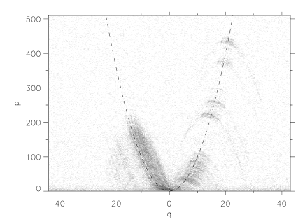
Figure 9: The secondary spectrum or PSR B0834+06 observed at 321 MHz on 2004 Jan 8 with the Arecibo telescope. The greyscale is logarithmic in relative power, with white being set 3 dB above the noise floor and black being set at 5 dB below maximum power. The arclet pattern seen prominently on the right hand side of the plot persisted for more than 25 days during 2004 Jan and moved systematically up and to the right along the guiding parabolic arc shown by the dashed line. The axis scaling is described in the text and can be compared directly with the plots of model data. The axes in this plot are scaled in the same way as in figure 8, but using the values $D_{p}=0.72{\rm kpc}$, ${\bf v}_{p}=175{\rm km\,s^{-1}}$, $\beta=0.33$, and $\theta_{o}\simeq 0.72\;{\rm mas}$.

The models in §4 were constructed to describe the effects of image speckle in the snapshot regime, and the evolution of the corresponding features in the secondary spectrum was discussed in §4.2. The timescale on which the arclets in B0834+06 change is observed to be very long, in some cases at least. In recent observations (Hill et al 2004), a persistent arclet pattern has been seen in B0834+06 for more than 25 days. (This is much longer than either the diffractive timescale, of 2 minutes, or the refractive timescale, of 2.6 days, for this pulsar at the observing frequency of 321 MHz.) Furthermore, the pattern shifts systematically in the direction from $-q$ to $+q$ in a linear fashion ($|\dot{q}|={\rm constant}$) at a rate consistent with the proper motion of the pulsar (${\bf v}_{\perp}\simeq(\beta-1){\bf v}_{p}$). These properties point to a phase profile that is localised in one region of the scattering screen and is scanned by the pulsar as it moves across the sky; this circumstance is consistent with the evolution expected in the case of a “frozen screen”, as discussed in §4.2. However, the large delays associated with the observed arclets (up to $300\;{\rm\mu s}$) require the phase coherence length to be as small as $s_{o}\sim 10^{9}\;{\rm cm}$, if they are caused by diffraction. If we assume that the characteristic velocity dispersion in the phase screen is $\sigma\ga c_{s}$, the sound speed, then with $c_{s}\sim 10\;{\rm km\,s^{-1}}$ we expect that individual stationary phase points should evolve on a time-scale $\la 10^{3}\,{\rm s}$. This is 1/2000 of (the lower limit on) their observed lifetime, and we conclude that the observed features cannot be attributed to isolated, individual image speckles,despite the superficial similarity of the data to figure 5. Instead these features must be attributed to either (i) a collection of many stationary phase points, if the corresponding image feature has a diffractive origin, or (ii) one or more stationary phase points associated with strong refraction. In the former case one can imagine that the physical cause might be a localised region of strong turbulence, in which the individual stationary phase points come and go; the lifetime of the secondary spectrum feature is then determined by the decay of the turbulence and may be much longer than that of any individual stationary phase point. On the other hand, if the feature is associated with strong refraction – i.e. a lens – then the relevant length scale in the phase screen is $\gg r_{F}\gg s_{o}$ and the corresponding timescale for evolution of the phase screen is naturally much longer. Indeed, in the case of a lens the phase structure need not be stochastic and might be in a quasi-steady state with no detectable evolution (e.g. Walker and Wardle 1998). In either case the image component must be tightly concentrated in order to avoid smearing the power over a range of delays (cf. figure 7). These compact refracting/scattering structures may be the same structures which are responsible for the Extreme Scattering Events (Fiedler et al 1987, 1994).

Despite the lack of agreement with the snapshot model, the results of §4 are useful in understanding the inverted arclets. A comparison of Figure 9 with Figures 5 and 6 indicates that the image must be highly elongated in order to produce the observed arclet pattern. This is a general result. No inverted arclet observations exist that are consistent with an axisymmetric image. Instead, the presence of inverted arclets is always accompanied by an absence of power in the $q=0$, $p>0$ region, and the vertices of the arclets lie along or very near a definite $p=\eta q^{2}$ locus, with $\eta$ constant over many years. All of these aspects follow naturally from an image that is highly elongated in one dimension and has numerous point-like features that self-interfere to give the observed arclets. Furthermore, the constancy of $\eta$ indicates that the region of the interstellar medium being probed has a consistent directionality associated with it, as would be produced by anisotropic scattering in the presence of a magnetic field (Higdon 1984, 1986; Goldreich & Sridhar 1995). This topic is explored further in Hill et al (2004).

One other insight emerges from a comparison between the models presented here and observations of scintillation arcs (e.g. Stinebring et al 2004). Interference between two identically scattered image components (e.g. Figure 7) is rare. Our modeling shows that the interference between two identically-scattered components would spread into a broad swath along the scintillation arc due to the wide range of differential delay values present. This is rarely seen in existing data, with thin arclets or pointlike interference features being much more common. This important item needs further exploration.

It is evident from the development in §§2–4 that secondary spectra encode information on the structure of radio images (i.e. radio-wave propagation paths) of pulsars. A great variety of structure is seen in observed secondary spectra, the vast majority of which remains to be decoded. Figures 5, 6 and 9 demonstrate that secondary spectra with thin arclets or other pointlike interference are particularly rich in information. Referring to equation 15, we see that $N$ points in the image should yield $N(N-1)/2$ features in the secondary spectrum. Consequently we have ${\cal O}(N^{2})$ constraints but only ${\cal O}(N)$ unknowns, so if $N\gg 1$ there is enough information to deduce the image structure from the observed secondary spectrum. Each stationary phase point (or point-like structure in the scattering screen) yields a measurement of the phase (up to an overall additive constant), phase gradient, and the combination of second derivatives which determines the magnification (eqs. 5–7); all of these quantities being determined at the location ${\bf x}_{i}$ of the image point. To the extent that the $N$ image points sample the image plane, these measurements therefore allow us to deduce the structure of the phase screen, $\phi$. We emphasise that this analysis does not require the assumption that the delays are purely geometric; the large number of available constraints should in fact provide powerful tests of any approximations which are used in the inversion. The main obstacle is observational: we require secondary spectra that show strong arclets or other sharply delineated interference features with good signal-to-noise ratio throughout. The data shown in figure 9 appear suitable, but we have not yet attempted the inversion.

7 Conclusions

Approximating the Fresnel-Kirchoff Integral by a sum over the stationary phase points of an arbitrary phase screen has allowed us to develop a probabalistic description of the power distribution in pulsar secondary spectra. We have presented a single-integral formulation of the power distribution for general axisymmetric images, and a closed form expression for highly anisotropic (i.e. linear) images. These results are descriptions of the (ensemble-)average properties, but our development makes it obvious how to generate examples of snapshot secondary spectra using the Monte Carlo method, and we have illustrated this technique with two examples. Our results clarify the origins of the parabolic arcs in observed secondary spectra, and provide an explanation for the inverted parabolic arclets which are also sometimes seen. The observed arclets are due to structured, highly elongated images. Long-lived arclets require correspondingly durable features in the phase-screen, and the data show that compact, isolated clumps of refracting/scattering material must exist in the interstellar medium. Consideration of the lifetime of highly anisotropic image components highlights an observational bias in favour of those which are elongated along the direction of the effective velocity vector.

8 Acknowledgments

We have benefitted greatly from helpful discussions with Barney Rickett and Jim Cordes.

Appendix A Evaluation of integrals for axisymmetric images

In evaluating the integral

$$P=\int d^{2}{\hbox{$\!\!$ $\mit\theta$}}_{1}d^{2}{\hbox{$\!\!$ $\mit\theta$}}_{2}\,p({\hbox{$\!\!$ $\mit\theta$}}_{1})p({\hbox{$\!\!$ $\mit\theta$}}_{2})\,\delta(p-{\hbox{$\!\!$ $\mit\theta$}}_{1}^{2}+{\hbox{$\!\!$ $\mit\theta$}}_{2}^{2})\delta(q-\theta_{1x}+\theta_{2x}),$$ (65)

one may assume $p\geq 0$ without loss of generality, with the function for $p<0$ determined from that for $p>0$ by $P(-p,q)=P(p,-q)$. For the axisymetric images under consideration here, the secondary spectrum is also symmetric in $q$, and in this Appendix we further limit the domain of our calculation to $q\geq 0$. One may carry out any two of the four integrals in eq. A.1 over the $\delta$-functions. We evaluate the integrals in polar coordinates, $d^{2}{\hbox{$\!\!$ $\mit\theta$}}_{i}=\theta_{i}d\theta_{i}d\psi_{i}$. Carrying out the integral over $d^{2}{\hbox{$\!\!$ $\mit\theta$}}_{1}$ gives

$$P(p,q)=\sum_{\pm}\int d^{2}{\hbox{$\!\!$ $\mit\theta$}}_{2}\,\left.{p({\hbox{$\!\!$ $\mit\theta$}}_{1})p({\hbox{$\!\!$ $\mit\theta$}}_{2})\over 2|\theta_{1y}|}\right|_{\theta_{1y}=\pm Y,\,\theta_{1x}=q+\theta_{2x}},$$ (66)

where $\theta_{1y}$ is determined by the $\delta$-functions, and is given by

$$Y^{2}=p+\theta_{2}^{2}-(q+\theta_{2}\cos\psi_{2})^{2}.$$ (67)

The boundary of the physical region is defined by $Y=0$. This corresponds to a parabola with apex at $\theta_{2x}=(p-q^{2})/2q$, and asymptotes at $\theta_{2y}\to\pm\infty$, $\theta_{2x}\to+\infty$. The integral is over the region outside this parabola. For $(p-q^{2})/2q>0$ the apex of the parabola is to the right of the origin, and the integral is over $0\leq\psi_{2}<2\pi$ for $\theta_{2}<(p-q^{2})/2q$, and over $\cos\psi_{2}\leq\cos\psi_{+}$, where

$$\cos\psi_{+}={{\sqrt{p+\theta_{2}^{2}}-q}\over{\theta_{2}}},$$ (68)

for $\theta_{2}>(p-q^{2})/2q$. For $(p-q^{2})/2q<0$ the apex of the parabola is to the left of the origin, so that a region around the origin is not in the range of integration, and the integral is over $\cos\psi_{2}\leq\cos\psi_{+}$ for $\theta_{2}>|(p-q^{2})/2q|$.

One procedure for evaluating the angular integral is to first change variables from $\psi_{2}$ to $t$, using

$$t=\tan{\psi_{2}\over 2},\qquad d\psi_{2}={2dt\over 1+t^{2}},\qquad\cos\psi_{2}={1-t^{2}\over 1+t^{2}}.$$ (69)

Then one finds

$$Y={{(p-q^{2}+2q\theta_{2})^{1/2}}\over{(1+t^{2})}}\left[\bigl{(}t^{2}+a^{2}\bigr{)}\bigl{(}t^{2}+b^{2}\right)\bigr{]}^{1/2},$$ (70)

where

$$a^{2}={\sqrt{p+\theta_{2}^{2}}+q+\theta_{2}\over\sqrt{p+\theta_{2}^{2}}+q-\theta_{2}},\quad b^{2}={\sqrt{p+\theta_{2}^{2}}-q-\theta_{2}\over\sqrt{p+\theta_{2}^{2}}-q+\theta_{2}}.$$ (71)

For $p>q^{2}$ and $0<\theta_{2}<(p-q^{2})/2q$ (with $q\geq 0$), we have $a^{2}>b^{2}>0$, while for $\theta_{2}>|(p-q^{2})/2q|$ we have $b^{2}<0<a^{2}$. Introducing $d^{2}=-b^{2}$, and making use of Gradshteyn and Ryzhik (1965: 3.152, 8.111.2, 8.112.1, 8.113.1) we find that the requisite integrals are

$$\int_{0}^{\infty}{dx\over[(a^{2}+x^{2})(x^{2}+b^{2})]^{1/2}}={1\over a}\,{\tenbi K}\left({\sqrt{a^{2}-b^{2}}\over a}\right),$$ (72)

and

$$\int_{d}^{\infty}{dx\over[(a^{2}+x^{2})(x^{2}-d^{2})]^{1/2}}={1\over\sqrt{a^{2}-b^{2}}}\,{\tenbi K}\left({a\over\sqrt{a^{2}-b^{2}}}\right),$$ (73)

where ${\tenbi K}$ is the Complete Elliptic Integral, with

$${\tenbi K}(k)={\pi\over 2}\left(1+{k\over 4}+\dots\right).$$ (74)

The foregoing results imply

$$\int_{0}^{\pi}{d\psi_{2}\over Y}={1\over{\sqrt{{\cal A}}}}{\tenbi K}\left(\sqrt{{\cal B}/{\cal A}}\;\right),$$ (75)

for $0<\theta_{2}<(p-q^{2})/2q$ (with $q\geq 0$), and

$$\int_{\psi_{2+}}^{\pi}{d\psi_{2}\over Y}={1\over{\sqrt{{\cal B}}}}{\tenbi K}\left(\sqrt{{\cal A}/{\cal B}}\;\right),$$ (76)

for $\theta_{2}\geq|(p-q^{2})/2q|$, where

$${\cal A}\equiv\left(\sqrt{p+\theta_{2}^{2}}+\theta_{2}\right)^{2}-q^{2}$$ (77)

and

$${\cal B}\equiv{4\theta_{2}\sqrt{p+\theta_{2}^{2}}}.$$ (78)

Substituting these results into equation A2 then yields our final result for the secondary spectrum corresponding to an axisymmetric image (equation 43).

References

- (1) Armstrong J.W., Rickett B.J., Spangler S.R. 1995 ApJ 443, 209
- (2) Cordes J.M., Rickett B.J., Stinebring D.R., Coles W.A. 2004 (In preparation)
- (3) Cordes J.M., Weisberg J.M., Boriakoff V. 1985 ApJ 288, 221
- (4) Ewing M.S., Batchelor R.A., Friefeld R.D., Price R.M., Staelin D.H. 1970 ApJL 162, L169
- (5) Fielder R.L., Dennison B., Johnston K.J., Hewish A. 1987 Nature 326, 675
- (6) Fielder R.L., Dennison B., Johnston K.J., Waltman E.B., Simon R.S. 1994 ApJ 430, 581
- (7) Goldreich P., Sridhar S. 1995 ApJ 438, 763
- (8) Goodman J., Narayan R. 1989 MNRAS 238, 995
- (9) Gradshteyn I.S., Ryzhik I.M. 1965 Table of integrals, series and products
- (10) Gupta Y., Rickett B.J., Lyne A.G. 1994 MNRAS 269, 1035
- (11) Gwinn C.R., Britton M.C., Reynolds J.E., Jauncey D.L., King E.A., McCulloch P.M., Lovell J.E.J., Preston R.A. 1998 ApJ 505, 928
- (12) Harmon J.K., Coles W.A. 1983 270, 748
- (13) Hewish A. 1980 MNRAS 192, 799
- (14) Hewish A., Wolzszczan A., Graham D.A. 1985 MNRAS 213, 167
- (15) Higdon J.C. 1984 ApJ 285, 109
- (16) Higdon J.C. 1986 ApJ 309, 342
- (17) Hill A.S., Stinebring D.R., Barnor H.A., Berwick D.E., Webber A. 2003 ApJ 599, 457
- (18) Hill A.S. et al 2004 (In preparation)
- (19) Lee L.C., Jokipii J.R. 1975 ApJ 201, 532
- (20) Lee L.C., Jokipii J.R. 1976 ApJ 206, 735
- (21) Melrose D.B, Macquart J.-P., Zhang C.M., Walker M.A. 2004 MNRAS (Submitted)
- (22) Narayan R., Hubbard W.B. 1988 ApJ 325, 503
- (23) Rickett B.J. 1990 ARAA 28, 561
- (24) Rickett, B.J., Lyne A.G., Gupta Y. 1997 MNRAS 287, 739
- (25) Roberts J.A., Ables J.G. 1982 MNRAS 201, 1119
- (26) Shishov V.I. 1974 Sov Astron AJ 22, 544
- (27) Stinebring D.R., McLaughlin M.A., Cordes J.M., Becker K.M., Espinoza Goodman J.E., Kramer M.A., Sheckard J.L., Smith C.T. 2001 ApJL 549, L97
- (28) Stinebring D.R. et al 2004 (In preparation)
- (29) Walker M.A., Wardle M.J. 1998 ApJL 498, L125
- (30) Wolszczan A., Cordes J.M. 1987 ApJL 320, L35