Strongest gravitational waves from neutrino oscillations at supernova core bounce

Abstract

Resonant active-to-active ($\nu_{a}\rightarrow\nu_{a}$), as well as active-to-sterile ($\nu_{a}\rightarrow\nu_{s}$) neutrino ($\nu$) oscillations can take place during the core bounce of a supernova collapse. Besides, over this phase, weak magnetism increases antineutrino ($\bar{\nu}$) mean free paths, and thus its luminosity. Because the oscillation feeds mass-energy into the target $\nu$ species, the large mass-squared difference between species ($\nu_{a}\rightarrow\nu_{s}$) implies a huge amount of energy to be given off as gravitational waves ($L_{\textrm{GWs}}\sim 10^{49}$ erg s^-1), due to anisotropic but coherent $\nu$ flow over the oscillation length. This asymmetric $\nu$-flux is driven by both the spin-magnetic and the universal spin-rotation coupling. The novel contribution of this paper stems from 1) the new computation of the anisotropy parameter $\alpha\sim 0.1-0.01$, and 2) the use of the tight constraints from neutrino experiments as SNO and KamLAND, and the cosmic probe WMAP, to compute the gravitational-wave emission during neutrino oscillations in supernovae core collapse and bounce. We show that the mass of the sterile neutrino $\nu_{s}$ that can be resonantly produced during the flavor conversions makes it a good candidate for dark matter as suggested by Fuller et al. (2003). The new spacetime strain thus estimated is still several orders of magnitude larger than those from $\nu$ difussion (convection and cooling) or quadrupole moments of neutron star matter. This new feature turns these bursts the more promissing supernova gravitational-wave signal that may be detected by observatories as LIGO, VIRGO, etc., for distances far out to the VIRGO cluster of galaxies.

I Introduction

Supernovae neutrinos and gravity waves.— That outflowing neutrinos ($\nu$s) from a supernova (SN) generate gravitational waves (GWs) was firstly pointed out by Epstein (1978). However, over the first $\sim 10$ milliseconds (ms) (Mayle, Wilson & Schramm 1987; Walker & Schramm 1987) after the SN core bounce the central density gets so high that no radiation nor even $\nu$s can escape, they are thus frozen-in and strongly coupled to the neutron matter ($N^{0}$) as described by the Lagrangean (see Kusenko & Postma 2002 for this dynamics)

$$L^{int}_{N^{0}\leftrightarrow\nu}=\frac{G_{F}}{\sqrt{2}}\left[\bar{N}^{0}\gamma_{\mu}(1-\gamma_{5})N^{0}\right]\left\{\bar{\psi}\gamma^{\mu}(1-\gamma_{5})\psi\right\}\;,$$ (1)

with the $\nu$ field $(\psi)$ satisfying the time-dependent Dirac equation

$$\left[i\gamma^{0}\partial_{0}+i\gamma^{\alpha}\partial_{\alpha}+\rho(t)v_{\beta}\gamma^{\beta}\left(\frac{1-\gamma_{5}}{2}\right)-m_{\nu}\right]\psi=0.$$ (2)

At this phase the whole proto-neutron star (PNS) dynamics is dominated by gravity alone, and can be appropriately described by the general relativistic Oppenheimer-Volkoff equation for both the $N^{0}$ + $\nu$ fluid (see Mosquera Cuesta 2002). As discussed by Mayle, Wilson & Schramm (1987); and Walker & Schramm (1987), it is over this early transient that most $\nu$ flavor conversions are expected to resonantly take place and consequently the super strong GWs burst from the oscillation process to be released. GWs from this decoupling has been suggested to likely be the ultimate process responsible for the neat kick given to a nascent pulsar during the SN collapse (Mosquera Cuesta 2000; 2002).

The contention of this paper is a) to pave, in the framework of general relativity (GR), the pathway to this fundamental astrophysical process of generation of GWs from $\nu$ oscillations in a PNS. b) to demonstrate, by taking into account experimental and observational constraints, that $\nu$ oscillations during SN core bounce do produce GWs of the sort predicted by Einstein’s GR theory, and more crucial yet, c) to stress that these bursts are the more likely SN GWs-signals to be detected by interferometric observatories as LIGO, VIRGO, GEO-600, etc. We speculate that such a signal perhaps might have been detected during the SN1987a event, despite the low sensitivity of the detectors at the time. Some claims in this direction were presented by Aglietta, Amaldi, Pizzella, et al.[2], and related papers.

II The mechanism for generating GWs during neutrino oscillations

To start with, let us recall how the production of GWs during $\nu$ oscillations proceeds by considering the case of oscillations between active and sterile neutrinos in the supernova core. The essential point here is that oscillations into sterile neutrinos change dramatically the energy and momentum (linear and angular) configuration of the system: neutrinos plus neutron matter inside the PNS (check Eq.(2)). In particular, flavor conversions into sterile neutrinos drive a large mass and energy loss from the PNS because once they are produced they freely escape from the star. The reason: they do not interact with any ordinary matter around, i.e., they do couple to active $\nu$ species but neither to $Z^{0}$ nor to $W^{\pm}$ vector bosons. This means that oscillations into steriles, in dense matter, take place over longer oscillation lengths, compared to $\nu_{a}\rightarrow\nu_{a}$, and the steriles encounter infinite mean free paths thereafter. Physically, the potential, $V_{s}(x)$, for sterile neutrinos in dense matter is zero. In addition, their probability of reconversion, still inside the star, into active species is quite small (see discussion below). This outflow translates into a noticeable modification of the PNS mass and energy quadrupole distribution, which as discussed below is dominated from the very beginning by rotational and magnetic field effects.

Since most steriles neutrinos escape along the directions defined by the dipole field and angular momentum vectors (see Fig.2), then the $\nu$ outflow is at least quadrupolar in nature. This produces a super strong gravitational-wave burst once the flavor conversions take place, the energy of which stems from the energy and momentum of the total number of neutrinos participating in the oscillation process. Further, the gravitational-wave signal generated this way must exhibit a waveform with a Christodolou’s memory (Mosquera Cuesta 2002).

The remaining configuration of the star must also reflect this loss. Hence, its own matter and energy distribution becomes also quadrupolar. Because this quadrupole configuration (the matter and energy still trapped inside the just-born neutron star) keeps changing over the time scale for which most of the oscillations take place, then GWs must be emitted from the star over that transient. At the end, the probability of conversion and the $\nu$ flux anisotropy parameter ($\alpha$, see below) determine both how much energy partakes in the process and the degree of asymmetry during the emission. Both characteristics are determine next.

EDITOR PLACE FIGURE 1 AROUND HERE !!!!!

The case for oscillations among active species is a bit different, the key feature being that mass and energy is relocated from one region to another inside the PNS, especially because of the weak magnetism of antineutrinos that allows them to have larger mean free paths (and thus oscillation lengths) (Horowitz 2002). In addition, oscillations of electron neutrinos into muon or tauon neutrinos leave these last species outside their own neutrinospheres, and hence they are in principle free to stream away. These neutral-current interacting $\nu$ species must be the very first constituents of the $\nu$ burst from any supernova since most $\nu_{e}$s are essentially trapped. This must also generate GWs during that sort of flavor conversions, although their specific strength (strain) must be a bit lower compared to conversions into sterile neutrinos where almost all the $\nu$ species may participate, and the large $\Delta m^{2}$ in the process.

Since the sterile neutrinos escape the core over a time scale of a few ms, the number of neutrinos escaping and their angular distribution is sensitive to the instantaneous distribution of neutrino production sites. Since thermalization cannot occur over such short times ($\Delta T^{\rm thermal}\sim 0.5$ s), and since the neutrino production rate is sensitive to the local temperature at the production site, the inhomogeneities during the collapse phase get reflected in the inhomogeneities in the escaping neutrino fluxes and their distributions. Because of both the $\nu$ spin-magnetic field ($\vec{B}$) and $\nu$ spin-angular momentum ($\vec{J}$) coupling the asymmetries in these distributions can give rise to quadrupole moments, which must generate gravitational waves as suggested by Mosquera Cuesta (2000; 2002), and dipole moments which can explain the origin of pulsar kicks (Kusenko & Segrè 1997; Fuller et al. 2003).

Fixed by the probability of oscillation, $P_{\nu_{a}\rightarrow\nu_{a}}^{\nu_{a}\rightarrow\nu_{s}}$, the fraction of neutrinos that can escape in the first few milliseconds is, however, small. Firstly, the neutrinos have to be produced roughly within one mean free path from their resonance surface. Secondly, since in the case of ${\nu_{a}\rightarrow\nu_{s}}$ oscillations $m_{s}$ is the heaviest neutrino species, the sign of the effective potential $A(x)$ (see discussion below) and the resonance condition indicates that only ${\nu}_{e}$s and the antineutrinos $\bar{\nu}_{\mu}$ and $\bar{\nu}_{\tau}$ can undergo resonant conversions. In Section IV we address all these issues and determine this fundamental property of the mechanism for producing GWs from $\nu$ flavor conversions.

III Anisotropic neutrino outflow: Origin and computation

To provide a physical foundation for the procedure introduced here to determine the neutrino asymmetry parameter, $\alpha$, which measures how large is the deviation of the $\nu$ flux from a spherical one, we recall next two fundamental effects that run into action once a PNS is forming after the supernova collapse. We stress that other physical process such as convection, thermalization, etc., are not relevant over the time scale under consideration: $\Delta T_{\rm osc}\sim 3-10$ ms after the SN core bounce. Those effects take a more longer time ($\sim 30-100$ ms) to start to dominate the physics of the PNS, and therefore do not modify in a sensitive manner the picture described below. Indeed, if $\nu$ thermalization, for instance, already took place, then the oscillations are severely precluded since oscillations benefit of the existence of energy, matter density and entropy gradients inside the PNS (Bilenky, Giunti and Grimus 1999; Akhmedov 1999), which are “washed out” once thermalization onsets.

EDITOR PLEASE PLACE TABLE 1 AROUND HERE !!!

A Why no room for $\nu$-driven convection over $\Delta T_{\rm osc}$

In order to back the dismissal in our discussion on neutrino oscillations of the effects of convection inside the proto-neutron star, we would like to take advantage of some arguments presented in the state-of-the-art of the subject by Janka, Kifonidis & Rampp (JKR, 2001), who provided detailed analysis about convection inside the nascent neutron star. In particular, these authors showed that the growth time scale of convective instabilities ($\tau_{\rm cv}$) in the neutrino-heated region (adjacent layers outside the just-born neutron star, of relevance for successful supernova explosions) depends on the gradients of entropy and lepton number through the growth rate of Ledoux convection, $\sigma_{L}$, as

$$\tau_{\rm cv}\simeq\frac{\ln(100)}{\sigma_{L}}\simeq 4.6\left[\frac{g}{\rho}\left(\frac{\partial\rho}{\partial s}\right)_{Y_{e},P}\frac{ds}{dr}+\left(\frac{\partial\rho}{\partial Y_{e}}\right)_{s,P}\frac{dY_{e}}{dr}\right]^{-1/2}\;,$$ (4)

or equivalently

$$\tau_{\rm cv}\simeq 20~{}{\rm ms}\left(\frac{R_{s}}{R_{g}}-1\right)^{1/2}\frac{R_{g,7}^{3/2}}{\sqrt{M_{1}}}\;;$$ (5)

where $M_{1}=1M_{\odot}$, and $R_{s}$ and $R_{g}$ define the shock and gain radius, respectively, and $R_{g,7}$ is a function of the gain radius, the temperature inside the star, and the neutrino luminosity and energy. Here the estimates were obtained for $g=GM/R_{g}^{2}$, $(\partial\rho/\partial s)_{P}\sim-\rho/s$, and $ds/dr\sim-\frac{1}{2}\frac{s}{(R_{s}-R_{g})}$ (see JKR 2001, for further details).

Numerical simulations demonstrate that convection inside the proto-neutron star does start as early as a few tens of milliseconds after core bounce. It develops in both ($i$) unstable surface-near regions, i.e., in layers around the neutrinosphere where density is $\rho\leq 10^{12}$ g cm^-3, and ($ii$) deeper layers of density $\rho\geq 10^{12}$ g cm^-3), where a negative lepton number gradient appears. Despite of this piece of evidence, the time scale defined by Eq.(5) is relatively long compared to both the estimated time interval for the deleptonization process to take place: $\Delta T_{\rm delept}\sim 10$ ms, i.e., time over which most electron neutrinos are produced (Mayle, Wilson & Schramm 1987; Walker & Schramm 1987), and the core bounce time scale: $\Delta T_{\rm bounce}\sim 20$ ms; where the large part of the neutrino luminosity associated with other flavors is produced through processes like bremsstrahlung, neutrino-neutrino and neutrino-nucleon scattering within less than 5 ms (Mayle, Wilson & Schramm 1987; Walker & Schramm 1987; JKR 2001, and references therein). Indeed, from the convective regions below the neutrinosphere neutron fingers dig into the star and reach its center in about one second. Then they propagate outwards to englobe almost all the exploding star. Under the physical conditions dominant over the first 10-20 ms after core bounce one expect most neutrino oscillations of all flavors to take place at that time. Thence, convective effects are not relevant during a time scale that short. As such, it cannot modify in a significant fashion our analysis regarding the mechanism for the generation of gravitational waves from neutrino oscillations, here highlighted.

Moreover, JKR (2001) stressed the “desastrous” rôle of rotation for convection. A high rotation velocity of the just-born neutron star reduces dramatically the effects of convection because of the suppression of the neutrino-nucleon interaction due to nucleon correlations in the nuclear medium composing the proto-neutron star. Physically, rotation leads to a suppression of convective motions near the rotation axis because of a stabilizing stratification of the star matter specific angular momentum. In passing, we stress that a similar effect is also expected from the action of a background magnetic field. Both effects, rotation and magnetic field, then appear to be more crucial for the physics of neutrino interactions inside the newly-born neutron star, and for the production of GWs during the oscillation transient. Thus we address both of them next.

B $\nu$-rotation interaction

That gravity couples to neutrinos is well-known since Dirac. The very first work, as far as we are aware of, to show that the particle spin and PNS rotation couples gravitationally, a universal feature (Soares & Tiomno 1996), was that of Unruh (1973). It was shown that a consistent minimal-coupling generalization to a curved background (a Kerr spacetime in that case) of the $\nu$ equations is possible, and that it leads to equations separable for the radial and angular components, though coupled. For a massless $\nu$ field (compare to Eq.(2)), and standard Minkowski space Dirac matrices $\gamma^{A}$, the Dirac equation derived by Unruh reads

$$\gamma^{A}\left(\frac{\partial}{\partial x^{A}}-\Gamma_{A}\right)\psi=0\;,\;\;\;$$ (6)

where the Dirac $\gamma^{A}$ matrices relate to the Kerr spacetime metric through

$$\gamma^{A}\gamma^{B}+\gamma^{B}\gamma^{A}=2g_{\rm Kerr}^{AB}\;.$$ (7)

Eq.(7) shows that the $\gamma^{A}$ matrices satisfy the Clifford’s algebra. Further, the spin-affine connections $\Gamma_{A}$ in Eq.(6) are uniquely determined by the relations

$$\Gamma_{A}\gamma^{B}-\gamma^{B}\Gamma_{A}=\frac{\partial\gamma^{B}}{\partial x^{A}}+\Gamma_{\alpha A}{{}^{B}\gamma^{\alpha}}\;,\;\;{\rm and}\;\;\;\;{\rm tr}(\Gamma_{A})=0\;.$$ (8)

From the $\nu$-number current, $J^{A}(x)=\bar{\psi}(x)\gamma^{A}\psi(x)$, it was shown that the $\nu$-number density is always positive and given as $(-g)^{1/2}J^{t}(x)=(-g)^{1/2}\bar{\psi}(x)\gamma^{t}\psi(x)$ (see Unruh 1973 for details). The complete analysis of the coupling shows that the $\nu$ field in this background is not superradiant, as opposed to the case of the classical fields studied previously.

Vilenkin (1978) extended the above analysis and showed that, upon admitting helicity ($L$) to be a good quantum number, the angular distribution $F_{jm}(\theta)$ of the thermal fermion gas of $\nu$s ($L=+1$) and $\bar{\nu}$s ($L=-1$) in the mode $(j,m)$, with the function $F_{jm}(\theta)$ satisfying the normalization condition $2\pi\int_{0}^{\pi}F_{jm}(\theta)\sin\theta d\theta=1$, leads to an asymmetric $\nu$ emission (see illustration in Fig.2) from a Kerr black hole (BH), of specific angular momentum $a\equiv J/M$, described by

$$\frac{dN}{dtd\omega d\theta}=\frac{1}{8\pi^{2}}M^{2}\omega^{2}\frac{\sum_{\pm}(1\pm La\cos\theta)}{\left\{e^{\left[\frac{2\pi}{k}(\omega\pm\frac{1}{2}\Omega_{BH})\right]}+1\right\}}\;.$$ (9)

Eq.(9) shows that more $\bar{\nu}$s are emitted in the direction parallel to the BH’s spin, whilst more $\nu$s escape in the antiparallel direction. Further, for other weak-interacting particles emitted from the BH parity is not conserved (Vilenkin 1978). More fundamental yet, Vilenkin (1978) work demonstrates that the same physics must be valid for any other rotating star. In other words, the $\nu$ spin coupling to rotation, in a gravitational background, is a universal feature, regardless which the spacetime source can be. Here onwards we shall take advantage of this feature for the case of neutrino emission from a rotating NS, and suggest that the basic quadrupole nature of the $\nu$ emission from the PNS stems in part from this spacetime effect. The other fundamental effect we address right next.

EDITOR PLEASE PLACE FIGURE 2 AROUND HERE !!!

C $\nu$-$B$ field interaction

That the electromagnetic properties of $\nu$s are modified due to its interaction with a background matter distribution is a well-known fact. This is reflected in the additional contribution to its self-energy stemming from the $\nu$ spin-to-magnetic field coupling $(\vec{B}\cdot\vec{k}_{\nu})$. In the case of $\nu_{\tau}\to\nu_{e}$ oscillations, for instance, the geometry of the $\nu$-sphere is dramatically deformed by $\vec{B}$ (see Fig.2), an effect that strongly depends upon the relative pointing directions of both $\vec{B}$ and $\nu$ momentum $\vec{k_{\nu}}$. The magnetic coupling distorts the $\nu_{\tau}$-surface (“sphere”) in such a way that it is no more concentric with the $\nu_{e}$-sphere (see Fig.1 and 2 in Kusenko 1999). Therefore, $\nu_{\tau}$s escaping paralelly-pointing to the $\vec{B}$ field have a lower temperature than those flowing away in the opposite (anti-parallel) direction.

At the same time, the $\nu$ spin coupling to rotation, Eq.(9) (Vilenkin 1978), drives also an effective momentum (and thus energy flux) asymmetry along the angular momentum direction $\vec{J}$, as shown in Fig.2. For a relative orientation $\theta(\vec{B}\leftrightarrow\vec{J})\neq 0$ between $\vec{B}$ and $\vec{J}$, i. e., a canonical pulsar, this combined action on the escaping $\nu$s of a rotating background spacetime plus magnetic field makes their $\nu$-sphere a decidedly distorted surface. More precisely, the volumetric region obtained by rotating around the hatched regions in Fig.2, becomes at least a quadrupolar outflowing energy distribution. This is the source of the strong GWs bursts in this mechanism when the oscillations ensue. It also justifies the large value of the anisotropy parameter $\alpha$ used in Eq.(14) below (see also Burrows & Hayes 1996).

EDITOR PLEASE PLACE TABLE 2 AROUND HERE !!!

D The anisotropy parameter

Based on the concommitant action of both effects: the $\nu$-spin coupling to both the magnetic field and rotation described previously, one can determine the $\nu$ flow anisotropy in a novel, self-consistent fashion by defining $\alpha$ as the ratio of the total volume filled by the distorted $\nu$-spheres to that of the proto-neutron star (PNS), as one can infer from Fig.2. The $\nu_{e}$-sphere radius of a non-magnetic non-rotating star is obtained from the condition:

$$\tau_{\nu_{e}}(R_{\nu_{e}})=\int_{R_{\nu_{e}}}^{\infty}{\mathcal{K}}_{\nu_{e}}~{}\rho(r)~{}dr=\frac{2}{3}\;,$$ (10)

where $\tau_{\nu_{e}}$ is the optical depth, and ${\mathcal{K}}_{\nu_{e}}$ the scattering opacity for electron neutrinos, and $\rho$ the matter density. Following Burrows, Hayes & Fryxell (1995) one can take hereafter $R_{\nu_{e}}\equiv R^{\nu_{e}}_{\rm PNS}\equiv R_{\nu}\sim 35$ km, which is of the order of magnitude of the oscillation length $\lambda_{\nu}$ of a typical supernova $\nu$, constituent as well of the atmospheric $\nu$s for which ${\Delta m^{2}}\sim 10^{-3}{\rm eV}^{2}$ has been estimated by Superkamiokande $\nu$ detector (Fukuda et al. 1998)

$$\lambda_{\nu}\sim 31~{}{\rm km}~{}\left[\frac{E_{\nu_{e}}}{10~{}{\rm MeV}}\right]\left(\frac{10^{-3}~{}{\rm eV}^{2}}{\Delta m^{2}}\right)\;.$$ (11)

Therefore, resonant conversions between active species may take place at the position $r$ from the center defined by

$$r=R_{\nu_{e}}+\delta_{0}\cos\phi\;,$$ (12)

with $\phi$ the angle between the $\nu$-spin and $\vec{B}$, i.e., $\cos\phi=\frac{(\vec{k}\cdot\vec{B})}{\vec{k}}$, and

$$\delta_{0}=\frac{e\mu_{e}B}{2\pi^{2}(dN_{e}/dr)}\sim 1-10~{}\rm km\;,$$ (13)

for $B\sim 10^{14-15}$ G, respectively. Here $e$, $N_{e}=Y_{e}N_{n}$ and $\mu_{e}$ represent the electron charge, density and chemical potential, respectively. This defines in Fig.2 an ellipsoidal figure of equilibrium with semi axes

$$a=R_{\nu}+\delta_{0};\hskip 14.22636pt{\rm and}\hskip 14.22636ptb=R_{\nu},$$ (14)

and volume (after rotating around $\vec{B}$):

$$V_{ellips.}=\frac{4}{3}\pi R^{2}_{\nu}(R_{\nu}+\delta_{0})\;.$$ (15)

Meanwhile, the $\nu$-spin coupling to rotation described by Eq.(9) generates an asymmetric lemniscate-like plane curve (see Fig.2)

$$r=R_{\nu}~{}(1\pm L~{}a~{}\cos~{}\theta)\;,$$ (16)

which upon a $2\pi$ rotation around the star angular momentum axis generates a volume:

$$V_{lemnisc.}=\frac{1}{4}(2R_{\nu})^{2}\times 2\pi\bar{y}+\frac{1}{4}(R_{\nu})^{2}\times 2\pi\bar{y}\;,$$ (17)

where the quantity $\bar{y}$ (and $\bar{x}$) is defined as the location of the centroid of one of the lobes of that plane figure with respect to its coordenate center (x,y), and is obtained from the standard definition $\bar{y}=\frac{\int ydA}{\int dA}$. After a long, but straightforward, calculation one obtains

$$\bar{y}=\frac{\sqrt{\pi}}{\Gamma^{2}(1/4)}~{}R_{\nu}\;,\hskip 14.22636pt\bar{x}=\frac{4\sqrt{\pi}}{\Gamma^{2}(1/4)}~{}R_{\nu}\;.$$ (18)

Thence, for a PNS as the one modeled by Burrows, Hayes & Frixell (1995), with parameters as given in Table II one obtains

$$\alpha_{\rm min}=\frac{V_{ellips.}+V_{lemnisc.}}{V_{\rm PNS}}\sim 0.11-0.01\;,$$ (19)

a figure clearly compatible with that one in Burrows & Hayes (1996). As such, this is essentially a new result of this paper. The attentive reader must notice in passing that the definition in Eq.(19) does take into account all of the physics of the neutrino oscillations: luminosity, density gradients and angular propagation, since Eqs.(12,16) do gather the relevant information regarding the spatial configuration of the $\nu$ luminosity in as much as is done in the standard definition of $\alpha$ (Burrows & Hayes 1996; Müller & Janka 1997)

$$\alpha(t)\equiv\frac{1}{L_{\nu}(t)}\;\int_{4\pi}d\Omega^{\prime}\;\Psi(\theta^{\prime},\phi^{\prime})\;\frac{L_{\nu}(\Omega^{\prime},t)}{d\Omega^{\prime}}\;.$$ (20)

Indeed, one can get the “flavour” of the relationship between these two definitions by noticing that the quantity $L_{\nu}(\Omega^{\prime},t)$ in the integrand of Eq.(20) can be expressed as $L_{\nu}(\Omega^{\prime},t)\equiv L_{\nu}(t)F(\Omega^{\prime})$, where the function $F(\Omega^{\prime})$ contains now all the information regarding the angular distribution of the neutrino emission. Hence $L_{\nu}(t)$ can be factorized out of the integral and dropped from Eq.(20). This converts Eq.(20) in a relationship among (solid) angular quantities, which clearly can be reduced to a volumetric one, similar to the one introduced in Eq.(19), upon a transformation using the definition of solid angle in the form of Lambert’s law: $d\Omega=\frac{dA\cos\theta}{R^{2}}$, and applied to the sphere representing the PNS. Here $\theta$, measured from a coordinate system centered at the PNS (source coordinate system in Müller & Janka 1997), plays the role of the angle between the direction towards the observer and the direction $\Omega^{\prime}$ of the radiation emission in Eq.(24), and subsequents, in Müller & Janka (1997). Therefore, the novel result here presented is physically consistent with the standard one for the asymmetry parameter $\alpha$.

IV Enlarged $\nu$ and GWs luminosity from oscillations in dense matter

$\nu$ outflow from a SN core bounce is a well-known source of GWs ( Epstein 1978; Burrows & Hayes 1996; Müller & Janka 1997; Mosquera Cuesta 2000; 2002). Numerical simulations (Müller & Janka 1997) showed that, in general, the fraction of the total binding energy emitted as GWs by pure $\nu$ convection is: $E^{\nu}_{\rm GW}\sim$ [10^-10-10^-13] M_⊙c², for a $\nu$ total luminosity: $L_{\nu}\sim 10^{53}$ erg s^-1.

Unlike GWs produced by $\nu$ convection (Müller & Janka 1997), in the production of GWs via $\nu$ oscillations (Mosquera Cuesta 2000; 2002) ($\nu_{a}\leftrightarrow\nu_{a}$ or $\nu_{a}\leftrightarrow\nu_{s}$) there exists two main reasons for expecting a major enhancement in the GWs luminosity during the transition: a) the conversion itself, which makes the overall luminosity ($L_{\nu_{x}}$) of a given $\nu_{x}$ species to grow by a large factor: $\Delta L_{\nu_{x}}\leq 10\%L^{\textrm{total}}_{\nu}$, see below. The enhancement stems from the mass-energy being given to, or drained from, the new $\nu$ species into which oscillations take place. This augment gets reflected in the species mass-squared difference, $\Delta m^{2}$, and their relative abundances: one species is number-depleted while the other gets its number enhanced. But, even if the energy increase, or give up, is small, b) the abrupt resonant conversion over the transition time (see Table I)

$$\Delta T_{\textrm{osc}}\equiv\frac{\lambda_{\textrm{osc}}}{\bar{V}_{\nu-Diff.}}\sim[10^{-4}-10^{-3}]~{}\rm s,$$ (21)

also magnifies transiently $L_{\nu_{x}}$. Here $\lambda_{\textrm{osc}}$ defines the oscillation length (computed below), and $\bar{V}_{\nu-Diff.}\sim 10^{9}$ cms^-1 the convective $\nu$ diffusion velocity (Müller & Janka 1997). In Section IV we estimate the transition probability: $P_{\nu_{a}\rightarrow\nu_{a}}(|\vec{x}-\vec{x}_{0}|)$, $P_{\nu_{a}\rightarrow\nu_{s}}(|\vec{x}-\vec{x}_{0}|)$, the quantity that measures how many $\nu$s can indeed oscillate. This probability also fixes the total amount of energy participating in the generation of the GWs through this mechanism, as shown in Section V.

If flavor transitions can indeed take place during supernovae (SNe) core collapse and bounce, then they must leave some imprints in the SNe neutrino spectrum. Main observational consequences of neutrino conversions inside SNe include a) the partial or total disappearance of the neutronization peak; the moment at which most $\nu_{e}$s are produced, b) the interchange of the original spectrum and the appearance of a hard $\nu_{e}$ spectrum, together with c) distorsions of the $\nu_{e}$ energy spectrum and d) alterations of the $\bar{\nu}_{e}$ spectrum (Dighe & Smirnov 2000). As discussed below in Section 4.4, observations of the neutrino burst from SN1987a have allowed to put some bounds on both $\nu_{a}\rightarrow\nu_{a}$ and $\nu_{a}\rightarrow\nu_{s}$ classes of flavor conversions.

A Resonance, adiabaticity and the role of weak magnetism

As argued by Mosquera Cuesta (2000; 2002) $\nu$ oscillations in vacuum produce no GWs. In the case of active-to-active $\nu$ oscillations (essentially the same physical argument holds also for active-to-sterile $\nu$ oscillations), the main reason for this negative result is that this class of conversions do not increase in a significant figure the total number of particles escaping from the proto-neutron star. In the case of active-to-active $\nu$ oscillations in dense matter, the process generates no GWs since the oscillations develop with the neutrinos having very short mean free paths, so that they motion outwards can be envisioned as a standard difussion process.

However, if one takes into account the novel result by Horowitz (2002) the situation may change dramatically. According to this author, because of the active antineutrino species weak magnetism their effective luminosity can be enlarged as much as 15% compared to the typical one they achieve when this effect is not taken into consideration during their propagation in dense matter. This result can be interpreted by stating that the number of oscillating (and potentially escaping) antineutrinos may be augmented by a large factor because now they do encounter longer mean free paths. Below we take advantage of this peculiar behaviour of $\nu$ outflow in supernovae in computing the overall probability of transition between active species and the GWs emitted in the process.

EDITOR PLEASE PLACE TABLE 3 AROUND HERE !!!

Wolfenstein (1978; 1979) and Mikheev & Smirnov (1985) pointed out that the neutrino oscillation pattern in vacuum can get noticeably modified by the passage of neutrinos through matter because of the effect of coherent forward scattering. Therefore, interaction with matter, as pictured by Eq.(1), may help in allowing more $\nu$s to escape if resonant conversions into active (Walker & Schramm 1987) and/or sterile $\nu$s (Mosquera Cuesta 2000) occur inside the $\nu$-sphere of the active $\nu$s.

The description of the two-neutrino oscillations process in matter follows from the Schrödinger-like (because the dynamics is described as a function of the space variable $x$ instead of the standard time $t$) differential equation (Bilenky, Giunti & Grimus 1999; Grimus 2003)

$$\displaystyle i\frac{{\rm d}}{{\rm d}x}\left(\begin{array}[]{c}a_{\alpha}\\ a_{\beta}\end{array}\right) = \displaystyle H^{\rm mat}_{\nu}\left(\begin{array}[]{c}a_{\alpha}\\ a_{\beta}\end{array}\right)$$ (26)

$$= \displaystyle\frac{1}{4E}\left\{\left[m_{1}^{2}+m_{2}^{2}+2\sqrt{2}G_{F}(N(\nu_{\alpha})+N(\nu_{\beta}))\right]\left(\begin{array}[]{cc}{1}&{0}\\ {0}&{1}\end{array}\right)\right.$$ (29)

$$+ \displaystyle\left.\left(\begin{array}[]{cc}A-\Delta m^{2}\cos 2\theta&\Delta m^{2}\cos 2\theta\\ \Delta m^{2}\cos 2\theta&-A+\Delta m^{2}\cos 2\theta\end{array}\right)\left(\begin{array}[]{c}a_{\alpha}\\ a_{\beta}\end{array}\right)\right\}\;,$$ (34)

where

$$A\equiv 2\sqrt{2}G_{F}E\left(N(\nu_{\alpha})-N(\nu_{\beta})\right),$$ (35)

and $N(\nu_{\alpha})\equiv\delta_{\alpha e}N_{e}-\frac{1}{2}N_{n}$, $\alpha,\beta=e,\mu,\tau,s$, $N(\nu_{s})=0$, and $\Delta m^{2}\equiv m_{2}^{2}-m_{1}^{2}$. The eigenfunctions of the matter effective Hamiltonian follow from the relation

$$H^{\rm mat}_{\nu}\psi_{mj}=E_{j}\psi_{mj}\;;$$ (36)

where

$$\psi_{m1}=\left(\begin{array}[]{c}\cos\theta_{m}\\ -\sin\theta_{m}\end{array}\right),\hskip 14.22636pt\psi_{m2}=\left(\begin{array}[]{c}\sin\theta_{m}\\ \cos\theta_{m}\end{array}\right).$$ (37)

The eigenvalues of $E_{j}$ and the matter mixing angle $\theta_{m}$ are thus given as

$$E_{1,2} = \left[m_{1}^{2}+m_{2}^{2}+2\sqrt{2}G_{F}(N(\nu_{\alpha})+N(\nu_{\beta}))\right]$$ (38)

$$\mp \sqrt{(A-\Delta m^{2}\cos 2\theta)^{2}+(\Delta m^{2}\sin 2\theta)^{2}}\;,$$ (39)

and

$$\tan 2\theta_{m}=\frac{\tan 2\theta}{1-\frac{A}{\Delta m^{2}\cos 2\theta}}\;,$$ (40)

where $\theta$ is the vacuum mixing angle. By defining $U_{m}(x)=(\psi_{m1},...,\psi_{mn})$ as the mixing matrix of $n$ $\nu$, and $\delta_{j}\equiv-i\int_{x_{0}}^{x_{1}}dx^{\prime}$ $\psi_{mj}(x^{\prime})^{\dagger}\psi_{mj}(x^{\prime})$ as the adiabatic phases, one can compute the oscillation amplitude as

$${\mathcal{A}}^{\rm adiab}_{\nu_{\alpha}\rightarrow\nu_{\beta}} = \sum_{j}U_{m}(x_{1})_{\beta j}~{}~{}exp\left(-i\left[\delta_{j}+\int_{x_{0}}^{x_{1}}dx^{\prime}E_{j}(x^{\prime})\right]\right)$$ (41)

$$\times U^{\star}_{m}(x_{0})_{\alpha j}\;.$$ (42)

Finally, by averaging over neutrino energies, i.e., by setting $\left\langle exp\left(-i\int_{x_{0}}^{x_{1}}dx^{\prime}\Delta E(x^{\prime})\right)\right\rangle_{\rm av}=0$ (see Bilenky, Giunti & Grimus 1999), the outcoming transition probability among active flavor-changing species thus reads

$$P_{\nu_{a}\rightarrow\nu_{a}}(|\vec{x}_{1}-\vec{x}_{0}|)=1-\frac{1}{2}\left[1+\cos 2\theta_{m}(x_{0})\cos 2\theta_{m}(x_{1})\right],$$ (43)

where $x_{0}$ and $x_{1}$ correspond to the production (emission) and detection sites, respectively.

B Active-to-active $\nu$ oscillations

As stated above, in order to produce an effect neutrinos must be able to escape the core without thermalizing with the stellar material. For active neutrino species of energies $\approx 10$ MeV, this is not possible as long as the matter density is $\geq 10^{10}$ g cm^-3. Since the production rate of neutrinos is a steeply increasing function of matter density (production rate $\propto\rho^{n}$, where $\rho$ is the matter density and $n>1$), the overwhelming majority of the neutrinos of all species produced are trapped. This way, there seems to be no contribution to the GWs amplitude for neutrino conversions taking place within the active neutrino flavors. In the first paper of this series (Mosquera Cuesta 2000), this difficulty was overcome only by addressing neutrino conversions into sterile species. Nonetheless, if there were indeed weak magnetism effects (Horowitz 2002), one can rethink conversions within active species. In his new result on weak magnetism for antineutrinos in core collapse supernovae, Horowitz (2002) showed that the antineutrinos ($\bar{\nu}_{x}$s) luminosity could be noticeably increased because of their longer mean free paths, and this means that the total energy flux can be augmented in $\sim 15\%$ for $\nu$s of temperature $\sim 10$ MeV. One can verify that longer mean free paths allows for a larger oscillation probability, and hence the contribution to the generation of GWs during flavor conversions within active species becomes nonnegligible compared to the earlier case (Mosquera Cuesta 2000) where not weak magnetism effects were taken into account.

For active-to-active $\nu$ flavor conversions, for instance: $\nu_{e}\rightarrow\nu_{\mu},\nu_{\tau}$; as implied by SNO results, the resonance must take place at a distance $x_{\rm res}$ from the PNS center and amid the active $\nu$-spheres, whenever the following relation is satisfied (see Table III)

$$\Delta m^{2}\cos 2\theta_{m}=2\sqrt{2}~{}~{}G_{F}~{}~{}N_{e}(x_{\rm res})~{}~{}k_{\nu_{e}}\;,$$ (44)

notice that we neglected the magnetic field contribution. Here $k_{\nu_{e}}=E_{\nu_{e}}/c$ is the $\nu_{e}$ momentum, and $N_{e}(x_{\rm res})=N_{e^{-}}-N_{e^{+}}\sim 10^{39-40}$ cm^-3 is the electron number density. Thus the right-hand part of this equation reduces to

$$2\sqrt{2}G_{F}E_{\nu_{e}}N_{e}(x_{\rm res})=6.9\times 10^{4}~{}{\rm eV^{2}}\left[\frac{\rho}{10^{11}\rm g~{}cm^{-3}}\right]\left(\frac{E_{\nu_{e}}}{\rm 10~{}MeV}\right)\;.$$ (45)

For densities of order $\rho_{x=x_{\rm res}}\sim 10^{10}$ g cm^-3, i.e., recalling that $\nu_{e}$s are produced at the PNS outermost regions (Walker & Schramm 1987) where the electron to baryon ratio is $Y_{e}\sim 0.1$, the resonance condition if satisfied for a mass-squared difference of about $\Delta m^{2}\sim 10^{4}$ eV², which implies a neutrino mass of about $m_{\nu}\sim 10^{2}$ eV. Neutrino flavor conversions in the resonance region can be strong if the adiabaticity condition is fulfilled (Walker & Schramm 1987), i.e., whenever (Bilenky, Giunti & Grimus 1999; Grimus 2003)

$$\frac{\Delta m^{2}\sin^{2}2\theta_{m}}{2E_{\nu}\cos 2\theta_{m}}\left(\frac{1}{\rho}\frac{{\rm d}\rho}{{\rm d}x}\right)^{-1}_{x=x_{\rm res}}\gg 1\;,$$ (46)

where $x_{\rm res}$ is the position of the resonance layer. Recalling that the typical scale of density variations in the PNS core is $h_{N_{e}}\sim(dN_{e}/dr)^{-1}\sim$ 6 km, this adiabatic behaviour could be achieved as far as the density and magnetic field remain constant over the oscillation length

$$\lambda_{\rm{osc}}\equiv\left(\frac{1}{\rho}\frac{{\rm d}\rho}{{\rm d}x}\right)^{-1}_{x=x_{\rm res}}\sim\left(\frac{1}{2\pi}\frac{\Delta m^{2}}{2k_{\nu}}\sin(2\theta_{m})\right)^{-1}\sim\frac{1~{}\rm cm}{\sin(2\theta_{m})}\;,$$ (47)

of order $h_{N_{e}}$, which can be satisfied for $\Delta m^{2}\sim 10^{4}$ eV² as long as (Kusenko & Segrè 1999)

$$\sin^{2}2\theta_{m}>10^{-8}\;.$$ (48)

Although these $\nu$ oscillations could be adiabatic for a wide range of mixing angles and thus a large number of $\nu$s could actually oscillate, a $\nu_{x}$ mass such as this is incompatible with both viable solutions to the Solar Neutrino Problem (SNP) and the most recent cosmological constraints on the total mass of all stable neutrino species that could have left their imprint in the Cosmic Microwave Background Radiation (CMBR), as inferred from the observations performed by the satellite WMAP: $m_{\nu}\sim 1$ eV. Therefore, we dismiss this possibility since there appears to be no evidence for neutrinos masses in this parameter range ($m_{\nu_{x}}\sim 10^{2}$ eV) inside the PNS core.

On the other hand, if one takes into account the KamLAND results (Eguchi et al. 2003), which definitively demonstrated that

$i$) a large mixing angle (LMA) solution of the solar $\nu$ problem is favoured: $\sin^{2}2\theta\sim 0.8$,

$ii$) for a mass-squared difference: $\Delta m^{2}\sim 5.5\times 10^{-5}$  eV² (we use the approximate value $\Delta m^{2}\sim 10^{-4}$ eV² for the estimates below),

one can see that resonant conversions with $\Delta m^{2}=m_{\nu_{2}}^{2}-m_{\nu_{1}}^{2}\sim 10^{-4}$ eV² would take place in supernova regions where the density is about $\rho\sim 10-30$ g cm^-3, which corresponds to the outtermost layers of the exploding star. Although a large number of $\nu$ species can in effect participate of the transitions there, i.e, the neutrino luminosity can be still a very large quantity, these regions are of no interest for the gravitational-wave emission from neutrino oscillations since the overall energy density at that distance from the star center is relatively small. This does not mean that no GWs are emitted from transitions there, it is to mean that their strain is very small so as to be detectable. As discussed by Dighe & Smirnov (2000), observations of $\nu$ oscillations in this parameter range would provide useful information regarding the SNP, the hierarchy of neutrino masses and the mixing $|U_{e3}|^{2}$. Note in passing that oscillations in this range would imply a mass for the $\nu_{2}$ species $m_{\nu_{2}}\sim 10^{-2}$  eV  $(\frac{\rho}{10~{}\rm g~{}cm^{-3}})$, in the case when $m_{\nu_{2}}>m_{\nu_{1}}$. This $m_{\nu_{2}}$ is compatible with current limits from WMAP (Pierce & Murayama 2003; Hannestad 2003).

Finally, let us consider oscillations in the parameter range estimated from CMBR by WMAP observations. In this case, resonant $\nu$ transitions would take place in regions where the density is as high as $\rho\sim 10^{7-8}$ g cm ^-3, that is, at the supernova mantle or PNS upper layers. At these densities the oscillation length can be still $\lambda_{\rm osc}\sim 1-5$ km, and thus the conversions can be considered as adiabatic. Thus the resonance condition can be satisfied for $\Delta m^{2}\sim 1$ eV² as long as $\sin^{2}2\theta_{m}\leq 10^{-3}$.

Hence, by plugging this constraint into Eq.(40), and recalling that $i$) at least 6 $\nu$-species can participate in the flavor transitions, $ii$) most $\nu$s are emitted having $\vec{k}_{\nu}$ parallel to $\vec{B}$, which implies a further reduction factor of 2, and also $iii$) most $\nu$s are emitted having $\vec{k}_{\nu}$ parallel to $\vec{J}$ implying an additional reduction factor of 2, one can show from Eq.(43) that the fraction of $\nu_{a}$ species that can eventually exchange flavor during the first few milliseconds after core bounce turns out to be (Mosquera Cuesta 2000)

$$P_{\nu_{a}\rightarrow\nu_{a}}(|\vec{x}-\vec{x}_{res}|)\sim 0.1~{}\%\;.$$ (49)

Thus, the total energy involved in the oscillation process we are considering could be estimated as: $E_{\nu}^{\rm tot}\simeq P_{\nu_{a}\rightarrow\nu_{a}}(|\vec{x}-\vec{x}_{res}|)\times N_{\nu}~{}k_{\nu}~{}c~{}(1+0.15)$, with $N_{\nu}$ the total number of neutrinos undergoing flavor conversions during the time scale $\Delta T_{\rm osc}$. This value leads to a bit stronger GW burst, as we show in Section V below.

Note in passing that KamLAND $\bar{\nu}_{e}$ experiment suggests $P_{\bar{\nu}_{e}\rightarrow\bar{\nu}_{\mu,\tau}}\sim 40\%$! (Eguchi, et al. 2003), while LSND $P_{\bar{\nu}_{\mu}\rightarrow\bar{\nu}_{e}}\sim 0.26\%$. This result from LSND has not been so far ruled out by any terrestrial experiment, and there is a large expectation that it could be verified by MiniBoone at Fermilab.

EDITOR PLEASE PLACE TABLE 4 AROUND HERE !!!

C Active-to-sterile $\nu$ oscillations

On the other hand, if the Liquid Scintillator Neutrino Detector (LSND) were a true indication of oscillations ($\bar{\nu}_{\mu}\leftrightarrow\bar{\nu}_{e}$) (Pierce & Murayama 2003; Hannestad 2003) with $\Delta m^{2}_{\rm LSND}\sim 10^{-1}$ eV², then active-to-sterile $\nu_{a}\rightarrow\nu_{s}$ oscillations could take place during a supernova core bounce (see Mosquera Cuesta 2002). Such oscillations would be resonant whenever the resonance condition is satisfied. As seeing from Table III this could happen for

$$\sqrt{2}G_{F}\left[N_{e}(x)-\frac{1}{2}N^{0}_{n}(x)\right]\equiv V(x)=\frac{\Delta m^{2}}{2E_{\nu}}\cos 2\theta_{m}\;.$$ (50)

Table III also shows that for $\nu_{\mu,\tau}\leftrightarrow\nu_{s}$ the $N_{e}$ term is absent, while in the case of $\bar{\nu}$s, the potential $V(x)$ changes by an overall sign. Numerically, for $\nu_{e}\leftrightarrow\nu_{s}$ oscillations

$$V(x)=7.5\times 10^{2}\left(\frac{\rm eV^{2}}{\rm MeV}\right)\left[\frac{\rho}{10^{10}\rm g~{}cm^{-3}}\right]\left[\frac{3Y_{e}}{2}-\frac{1}{2}\right]\;.$$ (51)

For $\nu_{\mu,\tau}\leftrightarrow\nu_{s}$ oscillations, the last term in parenthesis becomes $(\frac{Y_{e}}{2}-\frac{1}{2})\sim 1$.

$\nu$ conversions in the resonance region prove to be enhanced if the adiabaticity condition is fulfilled (Walker & Schramm 1987). This is the same as requiring the oscillation probability in Eq.(43) to become $P_{\nu_{a}\rightarrow\nu_{s}}=\cos^{2}2\theta_{m}\sim 1$. Moreover, after the resonance region the newly created sterile $\nu$s have very a small probability ($<P_{\nu_{s}\rightarrow\nu_{a}}>=\frac{1}{2}\sin^{2}2\theta_{m}$) of oscillating back to active $\nu$s, which could be potentially trapped. It is easy to check that the resonance condition in Eq.(50) is satisfied whenever

$$1~{}{\rm eV}^{2}\leq\Delta m^{2}_{{\nu}_{a}\rightarrow{\nu}_{4}}\leq 10^{4}~{}{\rm eV}^{2}\;.$$ (52)

Meanwhile, the adiabaticity condition, Eq.(46), holds if

$$\Delta m^{2}\frac{\sin^{2}2\theta_{m}}{\cos 2\theta_{m}}\gg 10^{-3}{\rm eV^{2}}\left(\frac{E_{\nu}}{10\rm MeV}\right),$$ (53)

since at the PNS core $\lambda_{\rm{osc}}\sim 1$ km (see Eq.(47)). This is easily satisfied for $\Delta m^{2}\leq 10^{4}$ eV² as long as $\sin^{2}2\theta_{m}\leq 10^{-7}$. This limit on the mixing angle is in agreement with Superkamiokande strong constraints on $\nu_{e}\rightarrow\nu_{s}$ mixing (Nunokawa 2001). Thence, we find that a substantial fraction ($P_{\nu_{a}\rightarrow\nu_{s}}\sim 1\%$) of $\nu$s may get converted to sterile $\nu$s, and escape the core of the star, if the sterile $\nu$ mass ($m_{\nu_{4}}$) is such that

$$1~{}{\rm eV}^{2}\leq\Delta m^{2}_{{\nu}_{a}\rightarrow{\nu}_{4}}\leq 10^{4}~{}{\rm eV}^{2}\;.$$ (54)

By looking at the lower limit for $\Delta m^{2}$ in Eq.(54) one can say that such a mass difference cannot solve the observed solar $\nu$ problem and/or being compatible with the atmospheric $\nu$ observations, but the possibility of having three light active $\nu$s of mass $m_{\nu_{1,2,3}}\sim[10^{-2}-10^{-3}]$ eV explaining these anomalies and a “heavy” sterile $\nu_{s}$ of mass $m_{\nu_{4}}\leq$ 1 eV as required by the LSND experiment remains to be a viable alternative. On the other hand, if the sterile neutrino could be as massive as $m_{\nu_{4}}\leq$ 1 keV this mass will make it a very promissing candidate as a constituent of the universe’s dark matter. This last possibility was recently readdressed by Fuller et al. (2003), who estimated sterile neutrino masses in the range (1-20) keV and small mixing angle $\sin^{2}2\theta\sim 10^{-4}$ with the electron neutrino as a potential explanation of pulsar kicks. The same argument had also been considered by Mosquera Cuesta (2002); and references therein.

As quoted above, for both classes of $\nu$ conversions the number of $\nu$s escaping and their angular distribution is sensitive to the instantaneous distribution of production sites. These inhomogeneities can give rise to quadrupole moments that generates GWs (Mosquera Cuesta 2000; Müller & Janka 1997), and dipole moments that could drive the runaway pulsar kicks (Kusenko & Segrè 1997; Fuller et al. 2003). Noting that at least 6 $\nu$-species can participate in both types of oscillations and that the interaction with both the magnetic field and angular momentum of the PNS brings with an overall reduction factor of 4 in the oscillation probability, one can show that the fraction of $\nu$s that can actually undergo flavor transitions in the first few milliseconds is (Mosquera Cuesta 2000)

$$P_{\nu_{a}\rightarrow\nu_{s}}^{\nu_{a}\rightarrow\nu_{a}}(|\vec{x}-\vec{x}_{0}|)\leq 1\%,$$ (55)

of the total $\nu$s number: M${}_{\odot}\times m_{p}^{-1}\sim 10^{57}\nu$, which corresponds to a total energy exchanged during the transition

$$\Delta E_{\nu_{a}\longrightarrow\nu_{s}}^{\nu_{a}\rightarrow\nu_{a}}\sim 3\times 10^{51}~{}\rm erg.$$ (56)

Equations (56,21) determine the total luminosity of the neutrinos participating in the resonant flavor conversions. These figures are called for in the definition used in Eq.(57) below, as the basis to compute the characteristic amplitude of the GWs emitted during the transitions discussed above.

The attentive reader must notice, however, that the lower limit in Eq.(52) stems from using the constraint derived from the observations of the CMBR performed by the satellite WMAP, which suggested that the total mass of all neutrino species should not be larger than $1$ eV. In a hierarchy where the heaviest $\nu$ is the sterile $\nu_{s}$, this limit leads to a maximum mass: $m^{\rm max}_{\nu_{s}}\sim 1~{}{\rm eV}$. The use of this mass-squared difference constraint implies that the density at the PNS region where the oscillations can take place is $\rho^{\rm WMAP}_{m_{\nu}}\sim 10^{8}$ g cm^-3. If the WMAP constraint on $m_{\nu}$ stands up also for sterile neutrinos, this would preclude the mechanism for giving to nascent pulsars the natal velocities (kicks) from active neutrino flavor conversions into sterile neutrinos, as claimed by Kusenko & Segrè (1997) and Fuller et al. (2003), since in such a case the transitions would take place in regions far outside the PNS core from where no influence could be received back once the oscillations develop. Nonetheless, the GWs emission would still take place, as we stressed above.

D Experimental bounds on supernova $\nu$ oscillations

Studies of SN physics have also focused on the potential rôle of oscillations (Walker & Schramm 1987) between active and sterile $\nu$s. In particular, there are limits on the $\nu_{e}\leftrightarrow\nu_{s}$ conversion rate inside the SN core from the detected $\nu_{e}$ flux from SN1987a (Nunokawa et al. 1997; Nunokawa 2001). According to (Nunokawa et al. 1997; Nunokawa 2001), the time spread and the number of detected $\nu_{e}$ events constrain $\nu_{e}\leftrightarrow\nu_{s}$ oscillations with: $10^{6}\leq\Delta m^{2}\leq 10^{8}{\rm eV}^{2}$ for $10^{-3}\leq\sin^{2}2\theta_{\nu_{e}\rightarrow\nu_{s}}\leq 10^{-7}$. More stringent constraints stem from arguing that if there were too many “escaping $\nu$s”, the SN explosion itself would not take place (Nunokawa et al. 1997; Nunokawa 2001). Such bounds are, however, model dependent. One should keep in mind that the mechanism through which the explosion takes place is, in fact, not well established (Buras, Rampp, Janka & Kifonidis 2003). In effect, it has been recently claimed that even after including all the best physics we know today about, i.e., the state-of-the-art on supernova physics, the numerical models of exploding stars do not explode as they should (Buras, Rampp, Janka & Kifonidis 2003). There seems to be a piece of missing physics in those formulations. Thence, there seems to be no hope of achieving $P_{\nu_{a}\rightarrow\nu_{s}}^{\nu_{a}\rightarrow\nu_{a}}$ larger than $\sim 1$% during $\nu$ oscillations in supernovae.

V GWs energetics from $\nu$ luminosity and Detectability

If $\nu$ oscillations do take place in the SN core, then the most likely detectable GWs signal should be produced over the time interval for which the conditions for flavor conversions to occur are kept, i. e., $\sim(10^{-1}-10)$ ms. This time scale implies GWs frequencies in the band: $f_{\rm{GWs}}\sim$ [10 - 0.1] kHz, centered at 1 kHz, because of the maximum $\nu$ production around $1-3$ ms after core bounce (see Walker & Schramm 1987). This frequency range includes the optimal bandwidth for detection by ground-based observatories. For a 1 ms conversion time span the $\nu$ luminosity reads

$$L_{\nu}\equiv\frac{\Delta E_{\nu_{a}\longrightarrow\nu_{s}}}{\Delta T_{\textrm{osc}}}\sim\frac{3\times 10^{51}\rm erg}{1\times 10^{-3}\rm s}=3\times 10^{54}\frac{\rm{erg}}{\rm s}\;.$$ (57)

Hence, the GWs luminosity, $L_{\textrm{GWs}}$, as a function of the $\nu$ luminosity can be obtained from the equation

$$\frac{c^{3}}{16\pi G}{\left|\frac{dh}{dt}\right|}^{2}=\frac{1}{4\pi R^{2}}L_{\textrm{GWs}}\;,$$ (58)

which relates the GWs flux to the GWs amplitude, $h_{\nu}$. In the case of GWs emission from escaping $\nu$s this amplitude is computed from the expression (Epstein 1978; Burrows & Hayes 1996; Müller & Janka 1997)

$$h_{ij}=\frac{2G}{c^{4}R}\int^{t-R/c}_{\infty}dt^{\prime}~{}~{}L_{\nu}(t^{\prime})~{}~{}\alpha(t^{\prime})~{}~{}e_{i}\otimes e_{j}\;,$$ (59)

where $e_{i}\otimes e_{j}$ represents the GWs polarization tensor.

To attain order of magnitude estimates one can transform Eq.(59) to get the amplitude of the GWs burst produced by the non-spherical outgoing front of oscillation-produced $\nu_{s}$ as (Mosquera Cuesta 2000; Burrows & Hayes 1996; Müller & Janka 1997)

$$h_{\nu} = \frac{2G}{c^{4}R}\left(\Delta t\times L_{\nu}\times\alpha\right)$$ (60)

$$h_{\nu} \simeq |A|\left[\frac{55\rm kpc}{R}\right]\left(\frac{\Delta T}{10^{-3}\rm s}\right)\left[\frac{L_{\nu}}{3\times 10^{54}\frac{\rm erg}{\rm s}}\right]\left(\frac{\alpha}{0.1}\right)\;,$$ (61)

where $|A|=4\times 10^{-23}~{}{\rm Hz}^{-1/2}$ is the amplitude. Equivalently, that amplitude can be reparametrized as

$$h_{\nu}\simeq|A|\left[\frac{55\rm kpc}{R}\right]\left(\frac{\Delta E_{\rm GWs}}{10^{-7}\rm M_{\odot}c^{2}}\right)^{1/2}\left[\frac{10^{3}\rm Hz}{f_{\rm GWs}}\right]^{1/2}~{}\;.$$ (62)

A GWs signal this strong will likely be detected by the first generation of GWs interferometers as LIGO, VIRGO, etc. Its imprint in the GWs waveform may resemble a spike of high amplitude and timewidth of $\sim$ ms followed by a Christodoulou’s memory (Mosquera Cuesta 2002). From Eq.(61) the GWs luminosity turns out to be

$$L_{\textrm{GWs}}\sim 10^{50-48}~{}~{}\frac{\rm{erg}}{\rm s}~{}~{}\left[\frac{L_{\nu}}{3\times 10^{54}\frac{\rm{erg}}{\rm s}}\right]^{2}\left(\frac{\alpha}{0.1-0.01}\right)^{2}\;,$$ (63)

while the GWs energy radiated in the process yields

$$E_{\textrm{GWs}}\equiv L_{\textrm{GWs}}\times\Delta T_{\textrm{osc}}\sim 10^{47-45}~{}{\rm erg}\;.$$ (64)

This is about $10^{5-3}\times L^{\rm Diff.}_{\nu}$ the luminosity from $\nu$ diffusion inside the PNS, as estimated earlier (Mosquera Cuesta 2000; 2002).

EDITOR PLEASE PLACE TABLE 5 AROUND HERE !!!

VI Conclusion

One can see that if $\nu$ flavor conversions indeed take place during SN core bounce inasmuch as they take place in our Sun and Earth (Smirnov 2002), then GWs should be released during the transition. The GWs signal from the process is expected to irradiate much more energy than current mechanisms figured out to drive the NS dynamics at birth do. A luminosity this large (Eq.(58)) would turn these bursts the strongest GWs signal to be detected from any SN that may come to occur, futurely, on distances up to the VIRGO cluster, $R\sim[10-20]$ Mpc. It is stressed that this signal will still be the stronger one from a given SN, even in the worst case in which the probability of $\nu$ conversion is three orders of magnitude smaller then the estimated in the present paper. In proviso, we argue that a GWs signal that strong could have been detected during SN1987a from the Tarantula Nebula in the Milky Way’s satellite galaxy Large Magellanic Cloud, despite of the low sensitivity of the detectors at the epoch. In such a case, the GWs burst must have been correlated in time with the earliest arriving neutrino burst constituted of some active species given off during the very early oscillation transient where some $\nu_{e}$s went into $\nu_{\mu}$s, $\nu_{\tau}$s or $\nu_{s}$s. Thenceforth, it could be of worth to reanalyze the data collected for from that event taking careful follow up of their arrival times, if appropriate timing was available at that moment.

VII Acknowledgements

The authors truly thank Profs. I. Damião Soares and R. Zukanovich Funchal for their patience in reviewing this manuscript and their valious criticisms and suggestions. HJMC acknowledges the support from the Fundação de Amparo à Pesquisa do Estado do Rio de Janeiro (FAPERJ), Brazil, through the grant E-26/151.684/2002. KF thanks CAPES (Brazil) for a graduate fellowship, Prof. Sandra D. Prado (IF-UFRGS) for continued support and advice, and ICRA-BR (Rio de Janeiro) for hospitality and support during part of this work.

EDITOR: THIS IS FIGURE 1 !!!!

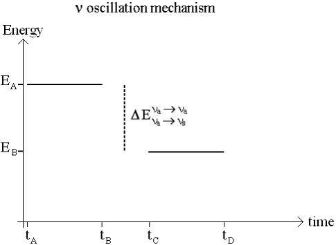
FIG. 1.: The mechanism for $\nu$ conversions. Firstly, the state of a system, $\nu$s in the PNS, is defined by the energy $E_{A}$ for the time interval $t_{B}-t_{A}$. After the flavor transitions that system is represented by a reduced energy $E_{B}$ over time $t_{D}-t_{C}$. The total energy transferred to the new species is $\Delta E_{\nu_{a}\leftrightarrow\nu_{a}}^{\nu_{a}\leftrightarrow\nu_{s}}\equiv E_{A}-E_{B}$, and thus the $\nu$ luminosity over the transient is given by $L_{\nu}=\frac{E_{A}-E_{B}}{t_{C}-t_{B}}$.

EDITOR: THIS IS FIGURE 2 !!!!

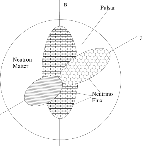
FIG. 2.: A schematic representation of the $\nu$-flux distribution (hatched regions) in a nascent pulsar. The at least quadrupolar distribution is evident and stems from the neutrino spin-magnetic and spin-rotation couplings.

EDITOR: THIS IS TABLE 1 !!!!

TABLE I.: Time scales (in ms) called for in this paper.

Supernova $\nu$	Neutrino	Supernova	Supernova
Thermalizat.	Oscillations	Deleptonizat.	Core-Bounce
$\Delta T_{\nu}^{\rm thermal}$	$\Delta T_{\rm osc}^{\nu}$	$\Delta T_{\rm delept}^{\rm PNS}$	$\Delta T_{\rm bounce}^{\rm PNS}$
$\sim 500$	$\sim 3-10$	$\sim 10$	$\sim 20$

EDITOR: THIS IS TABLE 2 !!!!

TABLE II.: Parameters of the PNS used for in this paper.

Radius	Mass	Density	$\nu$-sphere	Ang. Mom.
$R_{\rm PNS}$	$M_{\rm PNS}$	$\rho_{\rm PNS}$	$R_{\rm PNS}^{\nu}$	$a$
$\sim 80\rm~{}km$	$\sim 1.3~{}\rm M_{\odot}$	$3\times 10^{11}\rm g~{}cm^{-3}$	$\sim 35-60\rm~{}km$	$\sim 0.9-1$
		$2\times 10^{14}\rm g~{}cm^{-3}$

EDITOR: THIS IS TABLE 3 !!!!

ccccc $\nu_{e}\rightarrow\nu_{\mu,\tau}$ $\nu_{e}\rightarrow\nu_{s}$ $\nu_{\mu}\rightarrow\nu_{\tau}$ $\nu_{\mu,\tau}\rightarrow\nu_{s}$ $\frac{A}{2\sqrt{2}G_{F}E}$ $N_{e}$ $N_{e}-\frac{1}{2}N_{n}$ $0$ $-\frac{1}{2}N_{n}$

TABLE III.: Matter densities relevant for two-$\nu$ oscillations. Notice that $\nu_{\mu}\rightarrow\nu_{\tau}$ oscillations take place as in vacuum. The coupling Fermi constant is: $G_{F}^{2}=5.29\times 10^{-44}$ cm² MeV^-2, or equivalently $G_{F}=10^{-49}$ erg cm^-3.

EDITOR: THIS IS TABLE 4 !!!!

TABLE IV.: Parameter range for GWs emission from $\nu$s oscillations in SNe. The symbol DM stands for $\nu_{s}$ as a Dark Matter candidate.

$\nu$-sphere	$\nu$ Luminosity	Oscil. Length	$\nu$ Velocity	$\Delta m^{2}({\nu_{a}\leftrightarrow\nu_{a}})$	$\Delta m^{2}({\nu_{a}\leftrightarrow\nu_{s}})$	$\Delta m^{2}({\nu_{a}\leftrightarrow\nu_{s}})$
$R_{\rm PNS}^{\nu_{e}}$	$L({\nu-Diff.})$	$\lambda_{\rm osc}^{\nu}$	$\bar{V}_{\nu-Diff.}$	(SNO,KamLAND)	(WMAP)	($\nu_{s}$ DM)
$\sim 35$ km	$\sim 10^{53}\rm~{}erg~{}s^{-1}$	$\sim 1\rm~{}km$	$\sim 10^{9}\rm~{}cm~{}s^{-1}$	$\sim 10^{-4}\rm~{}eV^{2}$	$\sim 1\rm~{}eV^{2}$	$\sim 10^{4}\rm~{}eV^{2}$

EDITOR: THIS IS TABLE 5 !!!!

TABLE V.: GWs estimates from $\nu$ oscillations and diffusion.

GWs Freq.	GWs Energy	$L_{\nu}$ Asymm.	GWs Energy
$f_{\rm GW_{s}}$	$E_{\rm GW}(_{\nu_{a}\leftrightarrow\nu_{a}}^{\nu_{a}\leftrightarrow\nu_{s}})$	$\alpha$	$E_{\rm GW}({\nu-Diff.})$
$[10-0.1]\rm~{}kHz$	$[10^{-6}-10^{-8}]\rm~{}M_{\odot}~{}c^{2}$	$[0.1-0.01]$	$[10^{-10}-10^{-13}]\rm~{}M_{\odot}~{}c^{2}$

REFERENCES

- [1] Akhmedov, E. K. et al., 1999, Nuc. Phys. B 542, 3
- [2] M. Aglietta, et al., Nuovo Cim.C12, 75 (1989)
- [3] Arnett, W. D. & J. Rosner, Phys. Rev. Lett. 58, 1906 (1987)
- [4] Bilenky, S. M., Giunti, C. & Grimus, W. 1999, Prog. Part. Nucl. Phys., 43, 1-86
- [5] Buras, R., Rampp, M., Janka, H.-Th. & Kifonidis, K. 2003, Phys. Rev. Lett., 90, 241101; and report astro-ph/0303171 (v1): Improved models of stellar core collapse and still no explosions: What is missing ?
- [6] Burrows, A. & Lattimer, J., Astrophys. J. 251, 325 (1986)
- [7] Burrows, A. & Hayes, J. 1996, Phys. Rev. Lett., 76, 352
- [8] Burrows, A., Hayes, J. & Fryxell, B. A. 1995, ApJ, 450, 830
- [9] R. Cowsik, Phys. Rev. D 37, 1685 (1988)
- [10] Dighe, A. S. & Smirnov, A. Yu. 2000, Phys. Rev. D, 62, 033007
- [11] Eguchi, K. et al. 2003, [KamLAND Collaboration], Phys. Rev. Lett., 90, 021802
- [12] Epstein, R. I. 1978, MNRAS 188, 305
- [13] D. Fischer, Astron. Astrophys. 186, L11 (1987)
- [14] Fukuda, Y. et al., 1998, Phys. Rev. Lett., 81, 1562
- [15] Fuller, G. M., Kusenko, A., Mocioiu, I. & Pascoli, S. 2003, report astro-ph/0307267; to be published
- [16] Grimus, W. 2003, Neutrino Physics - Theory, report hep-ph/0307149 (v2)
- [17] Hannestad, S. 2003, report hep-ph/0302340 (v1)
- [18] M. Harwit, et al., Nature 328, 503 (1987)
- [19] Horowitz, C. J. 2002, Phys. Rev. D, 65, 043001
- [20] Janka, H-Th., Kifonidis, K. & Rampp, M. 2001, astro-ph/0103015 (v1)
- [21] Kusenko, A. private communication. Also Kusenko, A. 1999, report astro-ph/9903167
- [22] Kusenko, A. & Postma, M. 2002, Phys. Lett. B, 545, 238
- [23] Kusenko, A. & Segrè, G. 1997, Phys. Lett. B, 396, 197 —-. 1999, Phys. Rev. D, 59, 061302
- [24] L. C. Loveridge, Phys. Rev. D 69, 024008 (2004)
- [25] Mayle, R., Wilson, J. R., & Schramm, D. N. 1987, ApJ, 318, 288
- [26] Walker, T. P., Schramm, D. N., Phys. Lett. B 195, 331 (1987).
- [27] Mikheyev, S. P. & Smirnov, A. Yu. 1985, Yad. Fiz., 42, 1441; —-. 1985, Sov. J. Nucl. Phys., 42, 913
- [28] Mosquera Cuesta, H. J. 2002, Phys. Rev. D, 65, 061503(R) —-. 2000, ApJ, 544, L61
- [29] Müller, E. & Janka, H.-Th. 1997, A & A, 317, 140
- [30] Nunokawa, H. 2001, Nucl. Phys. Proc. Suppl., 95, 193
- [31] Nunokawa, H. et al., 1997, Phys. Rev. D, 56, 1704
- [32] Pantaleone, J., Phys. Lett. B 287, 128-132 (1992)
- [33] Pastor, S., Raffelt, G. G., Phys. Rev. Lett. 89, 191101 (2002)
- [34] Pierce, A. & Murayama, H. 2003, report hep-ph/0302131 (v1) (New neutrino mass constraints based on the Wilkinson Microwave Anisotropy Probe (WMAP))
- [35] Saha, D. & Chattopadhyay, G., Astrophys. Spac. Sc. 178, 209 (1991)
- [36] Samuel, S., Phys. Rev. D48, 1462 (1993)
- [37] Sato, K. & Suzuki, H., Phys. Rev. Lett. 58, 2722 (1987)
- [38] Spruit, H. & Phinney, E. S., Nature 393, 139 (1998)
- [39] Soares, I. D. & Tiomno, J. 1996 Phys. Rev. D, 54, 2808
- [40] Smirnov, A. Yu. 2002, Nuov. Cim., 117 B, N.9-11, 1237
- [41] Unruh, W. G. 1973, Phys. Rev. Lett., 31, 1265
- [42] Vilenkin, A. 1978, Phys. Rev. Lett., 41, 1575
- [43] Walker, T. P. & Schramm, D. N. 1987, Phys. Lett. B, 195, 331
- [44] Wolfenstein, L. 1978, Phys. Rev. D, 17, 2369 —-. 1979, Phys. Rev. D, 20, 2634