Diffuse inverse Compton and synchrotron emission
from dark matter annihilations in galactic satellites

Abstract

Annihilating dark matter particles produce roughly as much power in electrons and positrons as in gamma ray photons. The charged particles lose essentially all of their energy to inverse Compton and synchrotron processes in the galactic environment. We discuss the diffuse signature of dark matter annihilations in satellites of the Milky Way (which may be optically dark with few or no stars), providing a tail of emission trailing the satellite in its orbit. Inverse Compton processes provide X-rays and gamma rays, and synchrotron emission at radio wavelengths might be seen. We discuss the possibility of detecting these signals with current and future observations, in particular EGRET and GLAST for the gamma rays.

I Introduction

It is almost universally accepted that most of the matter in the universe is non-baryonic. This dark matter is the chief constituent of gravitationally bound objects from dwarf galaxy scales and larger. Identifying the nature of dark matter is one of the most important problems in astrophysics, cosmology, and particle physics.

Perhaps the best motivated candidate for cold dark matter is the lightest of the so–called neutralinos arising in supersymmetric extensions to the standard model jkg96 . These are the spin-1/2 Majorana fermion counterparts of the neutral gauge and Higgs bosons, and are expected to have masses at the weak scale (of order 100 GeV). This scale is intriguing as the relic density of a stable particle with this mass and corresponding cross section turns out to be of order the critical density, as we observe the matter density to be today. Any stable particles with weak scale masses could thus naturally account for the dark matter. In this paper, we will focus on supersymmetry, but our conclusions are fairly generic to dark matter candidates at the TeV scale.

We outline a new signature of annihilating dark matter in satellites of the Milky Way galaxy. Prospects for detecting high energy photons as dark matter annihilation products, primarily from the $\pi^{0}$ decays that are generic to hadronization processes, have been discussed for many years (for a sample see Ref. gammas ). Necessarily coming with these photons are high energy electrons and positrons from the analogous $\pi^{\pm}$ decay chains. Charged particles suffer complicated motions in the galactic magnetic field, and furthermore they lose energy to synchrotron and inverse Compton processes. Searching for the synchrotron emission from the galactic center syncGC and from galactic satellites blasi has been discussed previously, though neglecting the diffusion of the charged particles. We will show that the inverse Compton emission, extended over a large area from the charged particle annihilation products may be observable for some models of particle dark matter and of galactic satellites.

II Supersymmetric candidates

II.1 Particle physics model

In the Minimal Supersymmetric Standard Model (MSSM) the lightest of the superpartners (LSP) is often the lightest neutralino. The latter is a superposition of the superpartners of the neutral gauge and Higgs bosons,

$$\tilde{\chi}^{0}_{1}=N_{11}\tilde{B}+N_{12}\tilde{W}^{3}+N_{13}\tilde{H}^{0}_{1}+N_{14}\tilde{H}^{0}_{2}.$$ (1)

With R-parity conserved, this lightest superpartner is stable. For significant regions of the MSSM parameter space, the relic density of the stable neutralino is of the order $\Omega_{\chi}h^{2}\sim 0.1$, thus constituting an important (and perhaps exclusive) part of the cold dark matter. Note that $\Omega_{\chi}$ is the neutralino density in units of the critical density and $h$ is the present Hubble constant in units of $100$ km s^-1 Mpc^-1. Current observations, included those of the WMAP satellite and the Sloan Digital Sky Survey (we take the WMAP values), favor $h=0.71^{+0.04}_{-0.03}$ and a matter density $\Omega_{M}h^{2}=0.135^{+0.008}_{-0.009}$, of which baryons contribute a small amount $\Omega_{B}h^{2}=0.0224\pm 0.0009$ wmap ; sdss . If we assume that neutralinos are the only constituent of matter (neutrinos are a small contribution, $\Omega_{\nu}h^{2}<0.0076$), we can then infer $\Omega_{\chi}h^{2}=0.113^{+0.008}_{-0.009}$. We will apply a generous 3$\sigma$ constraint on the relic abundance from the WMAP data as follows: $0.086<\Omega_{\chi}h^{2}<0.137$.

Using the DarkSUSY code darksusy , we have explored the supersymmetric parameter space in both a phenomenological MSSM bg ; coann ; jephd ; bub ; neutrate ; other_db ; be99 ; sfermioncoann and in minimal supergravity (using the ISAJET code isajet ). Each model is subjected to current accelerator constraints on masses of superpartners and Higgs bosons pdg2002 ; lepsusy and on the $b\rightarrow s\gamma$ branching ratio cleo . Crucial for studies of dark matter, the relic abundance of neutralinos $\Omega_{\chi}h^{2}$ is calculated based on Refs. coann ; GondoloGelmini ; sfermioncoann .

II.2 Photon and electron spectra of annihilations

The only detailed information about models we require for this study (apart from the relic density constraint) is the annihilation cross section at non-relativistic velocities $\langle\sigma v\rangle$ (accounting for the factor of two due to identical particles in the initial state) and the spectrum of annihilation products, in particular the photons, electrons and positrons. The photons are primarily from the $\pi^{0}$ decays associated with hadronic final states, whereas the leptons can be from the associated $\pi^{\pm}$ decays, or more directly from massive gauge boson decays. In Fig. 1 we illustrate two models in the generic MSSM, one with a typical featureless spectrum of annihilation products, and the other clearly exhibiting the feature from $W^{\pm}$ decays.

Figure 1: Spectra of photons and leptons from annihilations in two characteristic models. The solid curves depict the combined electron and positron spectra, and the dotted curves show the photon spectra. Both of these models have acceptable values of $\Omega_{\chi}h^{2}$. The model on the left has an appreciable Higgsino fraction, and thus annihilates efficiently into $W$ pairs. The direct decays $W^{\pm}\rightarrow e^{\pm}\nu$ are responsible for the shelf in the lepton spectrum at energies right below maximum. The model on the right is a fairly pure gaugino, thus the final state is nearly always $q\overline{q}$, and the spectrum is featureless.

III Charged particle propagation and diffuse emission

The calculation of the diffuse emission from the annihilations proceeds in several steps. First, the time dependent density of charged particles is determined according to a diffusion model. The charged particles are trapped by the galactic magnetic field, which extends for several kpc from the stellar disk. Here we stress that we are concerned only with those galactic satellites that are currently (or in the recent past) within this “diffusion zone”. A time dependent treatment is necessary because a satellite moving with the typical galactic velocity of 300 km s^-1 crosses the diffusion zone in roughly one diffusion time: both timescales are of order tens of millions of years. The second step in the calculation is to calculate the column density of particles along various lines of sight, as a function of particle energy. Lastly, the inverse Compton and synchrotron spectra can be calculated from the particle spectrum under some assumptions about the galactic magnetic field and radiation fields.

III.1 Diffusion model

The propagation of charged particles in the tangled galactic magnetic field can be modeled as diffusion. Electrons and positrons lose energy rapidly to synchrotron radiation, and also to inverse Compton scattering on the cosmic microwave background (CMB) and on starlight. We will use the diffusion model of Ref. be99 . More sophisticated models are available, e.g. the semianalytic treatment of Ref. salati and the fully numerical GALPROP model galprop , but our model is simple to implement, yielding quantitatively similar results, and affords an intuitive understanding. We will make the assumption that the charged particle velocity distribution is locally isotropic, namely that the particles “stick” to the galactic magnetic field, and that the velocity distribution contains no record of the initial conditions. This is important as we consider sources (satellite halos) that move a significant distance in a diffusion time. If the velocity distribution was isotropic in the satellite frame (as could be the case if the satellite had a significant magnetic field of its own), our results would be different.

The time dependent diffusion–loss equation in homogeneous space for the density of charged particles as a function of energy $dn/dE$ is the following,

$$\frac{\partial}{\partial t}\frac{dn}{dE}=K(E)\nabla^{2}\frac{dn}{dE}+\frac{1}{E_{0}\tau}\frac{\partial}{\partial E}\left(E^{2}\frac{dn}{dE}\right)+Q,$$ (2)

where $K(E)=K_{0}3^{\alpha}[1+(E/3\;\rm GeV)^{\alpha}]$ is the energy dependent diffusion constant, with $K_{0}=3\times 10^{27}$ cm² s^-1 and $\alpha=0.6$. Energy loss due to any electromagnetic process where the exchanged energy is much less than $m_{e}c^{2}$ scales as $E^{2}$, and is proportional to the energy density in photons (or equivalently magnetic field). We consider synchrotron losses dues to a 3 $\mu$G galactic magnetic field (0.2 eV cm^-3), inverse Compton losses from the CMB (0.3 eV cm^-3), and inverse Compton losses due to starlight (0.6 eV cm^-3) longair . We thus set $dE/dt=E^{2}/(E_{0}\tau)$, with $E_{0}=1$ GeV, and $\tau=10^{16}$ s. Lastly, Q is the source function. Solving instead for $F=E^{2}\,dn/dE$, we find

$$\left(\frac{1}{E^{2}}\frac{\partial}{\partial t}-\frac{K(E)}{E^{2}}\nabla^{2}-\frac{1}{E_{0}\tau}\frac{\partial}{\partial E}\right)F\equiv{\cal L}F=Q.$$ (3)

We can calculate the Green function for this operator simply by 4-dimensional Fourier transform in $\vec{x}\rightarrow\vec{k}$ and $t\rightarrow\omega$,

$${\cal L}G=\delta^{3}(\vec{x}-\vec{x}^{\prime})\delta(t-t^{\prime})\delta(E-E^{\prime}) \rightarrow$$ (4)

$$\left[\frac{1}{E^{2}}\left(-i\omega+K(E)k^{2}\right)-\frac{1}{E_{0}\tau}\frac{\partial}{\partial E}\right]\tilde{G} = \frac{1}{(2\pi)^{4}}\,e^{i(\omega t^{\prime}+\vec{k}\cdot\vec{x}^{\prime})}\,\delta(E-E^{\prime}).$$ (5)

We should note that the Green function vanishes for $t^{\prime}>t$ and for $E^{\prime}<E$ because time increases monotonically, and energy decreases monotonically. This equation is easily solved for $E\neq E^{\prime}$:

$$\tilde{G}=\tilde{G}_{0}e^{i[\omega\tau(u-u^{\prime})-K_{0}\tau k^{2}(v-v^{\prime})]},$$ (6)

with $u=E_{0}/E$ and $v=3^{\alpha}u+u^{(1-\alpha)}/(1-\alpha)$. Hereafter we will denote the difference $X-X^{\prime}=\Delta X$ for some variable $X$. We now apply a jump condition to fix $\tilde{G}_{0}$: for $E>E^{\prime}$, $\tilde{G}=0$. The condition is

$$-\frac{1}{E_{0}\tau}\Delta\tilde{G}=\frac{1}{E_{0}\tau}\tilde{G}_{0}=\frac{1}{(2\pi)^{4}}e^{i(\omega t^{\prime}+\vec{k}\cdot\vec{x}^{\prime})},$$ (7)

and we thus derive the Fourier transform of the Green function,

$$\tilde{G}=\frac{E_{0}\tau}{(2\pi)^{4}}\,e^{i(\omega(\tau\Delta u+t^{\prime})+\vec{k}\cdot\vec{x}^{\prime}-K_{0}\tau k^{2}\Delta v)}.$$ (8)

Inverting the transform, we find the expected behavior that time and energy propagate in lockstep, yielding the free–space Green function

$$G_{\rm free}=\frac{E_{0}\tau}{(\pi D^{2})^{3/2}}\,e^{-\Delta\vec{x}^{2}/D^{2}}\,\delta(\Delta t-\tau\Delta u),$$ (9)

defining the effective diffusion length $D^{2}=4K_{0}\tau\Delta v=(3.550\;{\rm kpc})^{2}\Delta v$. This scale indicates that particles travel only a few kpc before losing most of their energy ($\Delta v\sim 1$).

The galactic magnetic field has a limited extent, which can be modeled simply by defining a diffusion zone at the boundary of which particles freely escape. Diffusion models typically require that the height of the diffusion zone is larger than $L=3$ kpc from the disk on both sides, and the radius is at least 20 kpc, and probably larger. For example the best GALPROP models galprop use $L=4$ kpc and a radius of 30 kpc. As the radial boundary is far from the Earth, we can safely neglect it in considering satellites within 10 kpc of us. We thus model the diffusion zone as an infinite slab of thickness $2L$, and we take $L=3$ kpc. We impose the boundary conditions that the density vanish at $z=\pm L$, which can be effected by a series of image charges at positions $x_{n}=x$, $y_{n}=y$, $z_{n}=(-1)^{n}z+2Ln$,

$$G_{2L}(\vec{x},\vec{x}^{\prime})=\sum_{n=-\infty}^{\infty}(-1)^{n}\,G_{\rm free}(\vec{x},\vec{x}^{\prime}_{n}).$$ (10)

The density of charged particles is now derived,

$$F=E^{2}\frac{dn}{dE}=\int_{R^{2}}d^{2}\vec{x}^{\prime}\int_{-L}^{L}\!\!\!dz^{\prime}\int_{-\infty}^{t}\!\!\!dt^{\prime}\int^{\infty}_{E}dE^{\prime}\,G_{2L}(\vec{x},\vec{x}^{\prime},t,t^{\prime},E,E^{\prime})\,Q(\vec{x}^{\prime},t^{\prime},E^{\prime}).$$ (11)

III.2 Diffuse emission: total power

For diffuse emission we are interested not in the local density of particles, but in the column depth of particles,

$$E^{2}\frac{d\sigma}{dE}=\int d\ell\,E^{2}\frac{dn}{dE}.$$ (12)

Placing the observer at the origin, at an angle $\delta$ from the galactic plane and an angle $\alpha$ from the line $y=0$, we find that for a distance $\ell$ from the observer,

$$x = \ell\,\cos\delta\,\cos\alpha,$$ (13)

$$y = \ell\,\cos\delta\,\sin\alpha,$$ (14)

$$z = \ell\,\sin\delta.$$ (15)

For simplicity we define $\hat{x}=\vec{x}/\ell$. The integral in $\ell$ can be applied directly to the free Green function, yielding the column depth at coordinates $(\alpha,\delta)$ due to a source at $\vec{x}^{\prime}$ (and we truncate at the edge of the diffusion zone, $\ell_{\rm max}=L/|\sin\delta|$),

$$G_{\rm free}^{\sigma}=\int_{0}^{\ell_{\rm max}}\!\!\!d\ell\,G_{\rm free}=\frac{E_{0}\tau}{2\pi D^{2}}e^{[(\hat{x}\cdot\vec{x}^{\prime})^{2}-\vec{x}^{\prime 2}]/D^{2}}\left[\mathop{\rm erf}\left(\frac{\ell_{\rm max}-\hat{x}\cdot\vec{x}^{\prime}}{D}\right)-\mathop{\rm erf}\left(\frac{-\hat{x}\cdot\vec{x}^{\prime}}{D}\right)\right]\delta(\Delta t-\tau\Delta u).$$ (16)

The Green function satisfying the boundary conditions is now simply

$$G_{2L}^{\sigma}(\alpha,\delta,\vec{x}^{\prime})=\sum_{n=-\infty}^{\infty}(-1)^{n}\,G_{\rm free}^{\sigma}(\alpha,\delta,\vec{x}^{\prime}_{n}),$$ (17)

and the column density of charged particles is

$$E^{2}\frac{d\sigma}{dE}=\int_{R^{2}}d^{2}\vec{x}^{\prime}\int_{-L}^{L}\!\!\!dz^{\prime}\int_{-\infty}^{t}\!\!\!dt^{\prime}\int^{\infty}_{E}dE^{\prime}\,G_{2L}^{\sigma}(\alpha,\delta,\vec{x}^{\prime},t,t^{\prime},E,E^{\prime})\,Q(\vec{x}^{\prime},t^{\prime},E^{\prime}).$$ (18)

We consider a toy model for dark matter clump undergoing annihilations. Assuming a very cuspy profile, most annihilations will occur very close to the center, and we can assume the clump is a point source. Taking the clump to be at position $\vec{X}=(X,Y,Z)$ today $(t=0)$, moving with constant velocity $\vec{V}$, we can write the source function as

$$Q(\vec{x},t,E)=\Gamma\frac{d\phi}{dE}\delta^{3}(\vec{x}-\vec{X}-\vec{V}t),$$ (19)

where $\Gamma$ is the annihilation rate in the clump, and $d\phi/dE$ is the spectrum of $e^{\pm}$ per annihilation. The delta functions simplify matters greatly, leaving only an integral in energy. The charged particle density (both $e^{+}$ and $e^{-}$) at the Earth and the column depth are given by

$$E^{2}\frac{dn}{dE}=\int_{E}^{\infty}dE^{\prime}\,\frac{d\phi}{dE^{\prime}}\frac{E_{0}\Gamma\tau}{(\pi D^{2})^{3/2}}\sum_{n=-\infty}^{\infty}(-1)^{n}e^{-\vec{w}_{n}^{2}/D^{2}}\,\theta\left(L-|w_{z}|\right),$$ (20)

$$E^{2}\frac{d\sigma}{dE}=\int_{E}^{\infty}dE^{\prime}\,\frac{d\phi}{dE^{\prime}}\frac{E_{0}\Gamma\tau}{2\pi D^{2}}\sum_{n=-\infty}^{\infty}(-1)^{n}e^{[(\hat{x}\cdot\vec{w}_{n})^{2}-\vec{w}_{n}^{2}]/D^{2}}\left[\mathop{\rm erf}\left(\frac{\ell_{\rm max}-\hat{x}\cdot\vec{w}_{n}}{D}\right)-\mathop{\rm erf}\left(\frac{-\hat{x}\cdot\vec{w}_{n}}{D}\right)\right]\theta\left(L-|w_{z}|\right).$$ (21)

The effective position $\vec{w}=\vec{X}-\vec{V}\tau\Delta u$, and $w_{z,n}=(-1)^{n}(Z-V_{z}\tau\Delta u)+2Ln$. We recover the steady–state solution by taking $\vec{V}=0$, indicating a source that has been at location $\vec{X}$ for all time.

We observe that looking at lower energies implies looking back in time, to when the source was in a different position. This leads to the formation of a “wake” of diffuse emission extending from the current position of the source (which will be a bright, concentrated source of gamma rays) in the direction it came from. The spatial signature is not unlike a comet, with a bright “nucleus” of gamma rays from the $\pi^{0}$ decays, and an extended tail of diffuse emission.

The energy loss time $\tau$ represents all energy loss mechanisms: inverse Compton scattering from both the CMB and starlight, and synchrotron emission. The total power emitted in any one of these is inversely proportional to the timescale for the individual process: $\tau_{\star}\approx 2\tau$, $\tau_{\rm CMB}\approx 4\tau$, and $\tau_{\rm sync}\approx 4\tau$. Integrating in energy,

$$P_{X}=\frac{1}{4\pi E_{0}\tau_{X}}\int dE\,E^{2}\frac{d\sigma}{dE},$$ (22)

and we note this has units power per area per solid angle. In Fig. 2 we illustrate contours of the total power in diffuse emission for several geometries of satellites. Finally, we note that the density of charged particles at the position of the Earth coming from the clump is typically unobservably small.

Figure 2: Total power in diffuse emission. The normalization is arbitrary; this figure is meant to illustrate the spatial extent of the signal. The contours are separated by 0.25 decade in power. Four satellite geometries are illustrated, each with a velocity of 300 km s^-1. The annihilation spectrum is that of the left panel of Fig. 1. In each case the current angular position is indicated with a cross. Top left: $(x,y,z)=(8,0,1)$ kpc, $\hat{v}=(0,5/13,12/13)$. In this case the clump has crossed more than half of the diffusion zone. Top right: $(x,y,z)=(12,0,4)$ kpc, $\hat{v}=(1,-1,1)/\sqrt{3}$. This illustrates the case where the clump has passed completely through the diffusion zone, leaving behind a wake that will dissipate shortly. A hint of the edge of the diffusion zone can be discerned at latitude $\approx 14^{\circ}$. Bottom left: $(x,y,z)=(8,0,2)$ kpc, $\hat{v}=(0,1,-1)/\sqrt{2}$. In this case the clump has recently entered the diffusion zone, thus the wake has not had much chance to form, and the diffuse flux drops very rapidly. Bottom right: $(x,y,z)=(8,2,0)$ kpc, $\hat{v}=(0,12,-5)/13$. This final panel depicts a clump moving nearly parallel to the galactic plane, thus the time spent inside the diffusion zone is relatively long, and the tail becomes more extended.

III.3 Diffuse emission: inverse Compton spectrum

For electrons of Lorentz factor $\gamma=E/m_{e}$ scattering from a blackbody spectrum of photons with $h\nu_{T}=kT$, the photon spectrum is given by the usual inverse Compton formula longair , integrated over the blackbody spectrum

$$\frac{1}{P_{X}}\frac{dP_{X}}{dx}=\frac{9}{128\zeta(3)}\,x^{2}\int_{0}^{4}\frac{dy}{y}\frac{2\ln(y/4)+1+4/y-y/2}{\exp(x/y)-1},$$ (23)

with $x=\nu/(\nu_{T}\gamma^{2})$. It is easy to show that this expression integrates to unity. This formula is inherently non-relativistic, implying that $\gamma h\nu_{T}\ll m_{e}c^{2}$. For the CMB, this is easily satisfied, as $h\nu_{T}=0.2348$ meV for a 2.725 K blackbody spectrum. For starlight, we assume a blackbody spectrum with $T=3800$ K icstar , thus $h\nu_{T}=0.33$ eV. The non-relativistic condition is satisfied for electron energies $E<$ TeV. This is true for most if not all of the annihilation products we will consider. We use $P_{X}=E^{2}/(E_{0}\tau_{X})$ to find the spectrum from a single particle (in power per frequency),

$$\frac{dP_{X}}{d\nu}=\frac{9}{128\zeta(3)}\,\frac{m_{e}^{2}}{E_{0}\tau_{X}\nu_{T}}\,x^{2}\int_{0}^{4}\frac{dy}{y}\frac{2\ln(y/4)+1+4/y-y/2}{\exp(x/y)-1}.$$ (24)

The spectrum from the full column of particles is then simply (in power per area per frequency)

$$\frac{dP_{X}}{d\nu}=\frac{m_{e}^{2}}{4\pi E_{0}\tau_{X}\nu_{T}}\int dE\,\frac{d\sigma}{dE}\,\left[\frac{1}{P_{X}}\frac{dP_{X}}{dx}\left(x=\frac{\nu m_{e}^{2}}{\nu_{T}E^{2}}\right)\right].$$ (25)

Detecting a diffuse signal in gamma rays will necessarily be hampered by at least the extragalactic background. The EGRET satellite measured this to be egretbg

$$E\,\frac{d\Phi}{dE}=(3.30\pm 0.15)\times 10^{-6}\left(\frac{E}{0.451\;\rm GeV}\right)^{-1.10\pm 0.03}\rm cm^{-2}\;s^{-1}\;sr^{-1}.$$ (26)

III.4 Diffuse emission: synchrotron spectrum

The total power in synchrotron radiation is similar to that in inverse Compton emission in that both are proportional to $E^{2}$. The spectra are different however.

$$\frac{1}{P_{\rm sync}}\frac{dP_{\rm sync}}{dx}=\frac{27\sqrt{3}}{32\pi}\,x\int_{0}^{\pi}d\alpha\,\sin\alpha\int_{x/\sin\alpha}^{\infty}dy\,K_{5/3}(y),$$ (27)

and now $x=\nu/(\nu_{B}\gamma^{2})$, with $\nu_{B}=3eB/(4\pi m_{e}c)=12.6\,(B/3\mu\rm G)$ Hz. This is just the usual synchrotron formula, isotropically integrated over the angle the particle trajectory makes with the magnetic field. It is again easy to show that this expression integrates to unity. The spectrum from the full column of particles is then easily recovered from Eq. 25, replacing the $(dP/dx)/P$ with the synchrotron formula, and replacing $\nu_{T}$ with $\nu_{B}$ (and we take $B=3\mu$G). The chief diffuse background for this synchrotron signal is the CMB, which peaks at 160 GHz. At 1 GHz, the power is $2.09\times 10^{4}$ Jy sr^-1. In Fig. 3 we plot the spectra of inverse Compton and synchrotron emission from a line of sight that is 5 degrees behind the current position of a clump. We will neglect complications such as synchrotron self-absorption and synchrotron self-Compton processes as we calculate the photon density to be much smaller than in previous treatments blasi due to the diffusion of the source electrons.

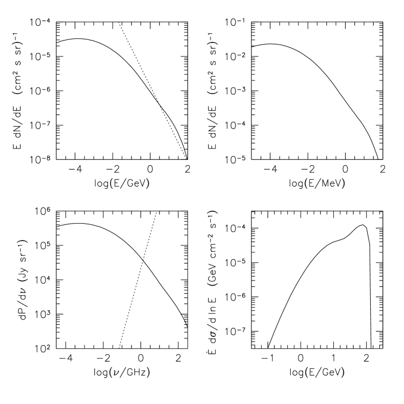
Figure 3: Spectra of diffuse emission in inverse Compton and synchrotron radiation. The clump is located at $(x,y,z)=(8,0,1)$ kpc, with a velocity of 300 km s^-1 in the $\hat{v}=(0,5/13,12/13)$ direction, as in the top left panel of Fig. 2. The annihilation spectrum is that of the left panel of Fig. 1. The line of sight illustrated trails the current location of the clump by 5 degrees in the $-\hat{v}$ direction. The total annihilation rate is 10³⁹ s^-1. Top left: Spectrum of inverse Compton emission from interactions with starlight, assuming an energy density of 0.6 eV cm^-3 with a 3800K blackbody spectrum. The dotted curve is the diffuse gamma ray background. Top right: Inverse Compton on the CMB. Bottom left: Synchrotron emission assuming a 3 $\mu$G magnetic field. The dotted curve is the CMB. Bottom right: Column depth of particles as a function of energy, weighted by the energy loss rate. It is clear that most of the diffuse power is radiated by relatively high energy particles.

IV Galactic halo substructure

Many authors have discussed the distribution of substructure in galactic halos. There are two important issues relating to the detectability of annihilations in these structures, both their mass distribution and their density profile. Again we stress that we are interested only in those satellites within the diffusion zone. As the diffusion zone is fairly extended, there should be a significant number of such satellites: even out to a radius of 30 kpc, the diffusion zone is roughly 15% of the total volume of the galactic halo.

IV.1 Density profiles

We first discuss the density profiles of the satellite halos that we hope to detect. Numerical N-body simulations find that structures at all scales diverge as a power law at small radii. In particular, the popular NFW profile nfw is given by

$$\rho(r)=\rho_{0}\left(\frac{a}{r}\right)\frac{a^{2}}{(a+r)^{2}}.$$ (28)

These profiles can be normalized according to simulations, based on the virial mass and radius, where the density is roughly 340 times the cosmological density (for the concordance model) $\rho_{c}=3\Omega H_{0}^{2}/8\pi G\approx 1.4\times 10^{-6}\,\rm GeV\;cm^{-3}$. The relevant parameter is the concentration $C=r_{\rm vir}/a$, with $r_{\rm vir}=260(M_{\rm vir}/10^{12}\,M_{\odot})^{1/3}\,{\rm kpc}$ concentration , finding

$$C \approx 107\left(\frac{M_{\rm vir}}{M_{\odot}}\right)^{-0.084},$$ (29)

$$\rho_{0} = 340\,C(1+C)^{2}\rho_{c},$$ (30)

$$M_{\rm vir} = 4\pi\rho_{0}\left(\frac{r_{\rm vir}}{C}\right)^{3}\left[\ln\left(1+c\right)-\frac{C}{1+C}\right].$$ (31)

The specific annihilation rate is then given by

$$\frac{\Gamma}{M_{\rm vir}}=\frac{\langle\sigma v\rangle\rho_{0}}{3m^{2}}\frac{1-(1+C)^{-3}}{\ln(1+C)-C/(1+C)}\rightarrow\frac{\langle\sigma v\rangle\rho_{0}}{3m^{2}}\frac{1}{\ln C-1}\;\;(C\gg 1).$$ (32)

The Moore profile has a steeper central cusp with a divergent total flux moore . Thus a minimum radius $r_{\rm min}$ needs to be defined to regularize. The profile is given by

$$\rho(r) = \rho_{0}\left(\frac{a}{r}\right)^{1.5}\frac{1}{[1+(r/a)^{1.5}]},$$ (33)

$$\frac{\Gamma}{M_{\rm vir}} \rightarrow \frac{\langle\sigma v\rangle\rho_{0}}{m^{2}}\frac{\ln(a/r_{\rm min})}{\ln C}.$$ (34)

For cusps $\rho\propto r^{-\alpha}$ steeper than $\alpha=1.5$, we find the behavior (with the proper limit as $\alpha\rightarrow 1.5$)

$$\frac{\Gamma}{M_{\rm vir}}\rightarrow\frac{\langle\sigma v\rangle\rho_{0}}{m^{2}}\frac{(a/r_{\rm min})^{2\alpha-3}-1}{(2\alpha-3)\ln C}.$$ (35)

IV.2 Mass distribution of subhalos

Simulations indicate that the mass distribution of subhalos is a power law, given by

$$N\propto\left(\frac{M}{M_{\rm vir}}\right)^{-\alpha},$$ (36)

with a normalization that about 500 clumps with masses larger than $10^{8}\,M_{\odot}$ are found in a halo like that of the Milky Way clumpspectrum . This means that there will be only a handful of clumps more massive than $10^{10}\,M_{\odot}$. At $M_{\rm vir}=10^{9}\,M_{\odot}$, the concentration is $C\approx 19$. The specific annihilation rate for a clump is easily determined, using $\langle\sigma v\rangle\rho_{c}/m^{2}=5\times 10^{24}\,(\langle\sigma v\rangle/10^{-27}\,{\rm cm^{3}\;s^{-1}})\,(m/{\rm GeV})^{-2}\,M_{\odot}^{-1}\,\rm s^{-1}$. Using $\rho_{0}\approx 340\rho_{c}C^{3}$ for any of these halo models, we can find a simple expression for the total annihilation rate in a “large” clump, defined as $M_{\rm vir}=10^{9}\,M_{\odot}$, $r_{\rm vir}=26$ kpc (and $a=1.4$ kpc):

$$\Gamma_{\rm NFW} = 2\times 10^{39}\,\frac{\langle\sigma v\rangle_{27}}{m^{2}_{\rm GeV}}\;\rm s^{-1},$$ (37)

$$\Gamma_{\alpha} = 4\times 10^{39}\,\frac{(a/r_{\rm min})^{2\alpha-3}-1}{2\alpha-3}\,\frac{\langle\sigma v\rangle_{27}}{m^{2}_{\rm GeV}}\;\rm s^{-1}.$$ (38)

In supersymmetric models, $\langle\sigma v\rangle_{27}/m^{2}_{\rm GeV}<10^{-2}$. The Moore profile has a logarithmically diverging flux, but the enhancement factor is less than 40 if annihilations empty the central cusp, and much less than that for other mechanisms. For example, if interactions with a central black hole sweep out the central region (of order 1 pc), the enhancement is less than 10. This may be the case for the full galactic halo, but for dark clumps without stars, there may be no central black hole. Steeper profiles can in principle have much larger enhancement factors, though with a cutoff of 1 pc, the enhancement is less than of order 1000 even for $\alpha=2$. In the next section, we will see that annihilation rates of order $10^{38}\,\rm s^{-1}$ are needed for point sources to be confidently seen in diffuse emission, thus $\alpha\geq 1.5$ is probably required. Coincidentally, steeper profiles look more like point sources, so clumps with high enough annihilation rates will be easy to model from this perspective. However, the NFW profile is not too far from detectability for a 10${}^{9}M_{\odot}$ clump, if the annihilation cross section is the maximum allowed. Some clumping of the halo might tip the balance and make even this profile a candidate for detection in inverse Compton emission. Here we note that the effect that clumpiness in galactic halos has on dark matter detection has been discussed at length, e.g. Ref.clumping .

V Unidentified EGRET sources

The EGRET gamma ray survey discovered a large number of point sources, a large fraction of which remain unidentified egretpoint . These sources typically have fluxes of order

$$E\,\frac{d\Phi}{dE}\sim 10^{-8}\left(\frac{E}{\rm GeV}\right)^{-1}\,{\rm cm^{-2}\;s^{-1}}.$$ (39)

We investigate the possibility that some of these might be Milky Way satellites undergoing annihilations at their centers. The annihilation scenario requires that there is no other concentrated emission than the gamma rays. Other astrophysical sources of just about any type are expected to have emission at other wavelengths as well. These sources (identified or not) are not measured below about 100 MeV, thus the turnover expected for $\pi^{0}$ photons at $m_{\pi^{0}}/2=67.5$ MeV could not have been observed. However, the spectrum of an annihilation source should be closer to flat around 100 MeV, as seen from Fig. 1, thus the EGRET point sources are typically not very good candidates for annihilation radiation. However, they do set the scale of possible annihilation sources quite well.

The yield of gamma rays predominantly from $\pi^{0}$ decays in the hadronization of annihilation products is typically $dN/d\,\ln\,E\sim 2$ annihilation^-1 at energies of $0.1$ GeV. This means the inferred rate of annihilations for these sources is $5\times 10^{-8}$ cm^-2 s^-1. For a clump at a distance of 8 kpc, the inferred annihilation rate is $4\times 10^{38}$ s^-1. As we have seen in the previous section, this rate likely requires a central density cusp at least as steep as $r^{-1.5}$.

We ask the following question: can GLAST confirm or rule out the hypothesis that some of the unidentified EGRET point sources are the annihilating cores of very steep profile dark matter subhalos? We argue that the answer is yes, for two reasons. First, GLAST will have improved performance an energies below 100 MeV, down to a threshold of 20 MeV. Certainly, the turnover in spectrum at about 70 MeV that should be present in an annihilation source should be visible. Second, the diffuse inverse Compton emission associated with a few times 10³⁸ annihilations per second, covering hundreds of square degrees, should yield both a significant fraction of the background and a statistically significant detection. GLAST will have an enormously improved exposure over EGRET: at 1 GeV and above, the expectation is $4.5\times 10^{10}$ cm² s to any point on the sky, per year glastexposure . In Fig. 4, we illustrate the integrated flux from inverse Compton on starlight in four energy intervals due to an annihilation source of $4\times 10^{38}$ s^-1 with the spectrum of the left panel of Fig. 1. We find that such a source should be easy for GLAST to detect, in fact a source ten times less active, with $4\times 10^{37}$ annihilations per second should be detectable. These results are summarized in Table. 1.

Energy	Size (68%)	S / BG	BG (EGRET)	BG (GLAST)	S/N (EGRET)	S/N (GLAST)
(GeV)	(sr)		(counts)	(counts)
0.03 – 0.1	0.078	0.551	250.	5,630	8.72	41.4
0.1 – 0.3	0.084	0.961	75.2	4,230	8.33	62.5
0.3 – 1	0.093	1.447	23.6	2,650	7.03	74.6
1 – 3	0.102	2.098	7.25	1,630	5.65	84.8
3 – 10	0.102	3.209	2.06	463.	4.60	69.0
10 – 30	0.076	5.322	0.43	97.1	3.49	52.4
30 – 100	0.042	8.019	0.07	15.1	2.08	31.2
100 – 300	0.021	6.562	0.01	2.10	0.63	9.50

Table 1: Detectability of diffuse inverse Compton emission in EGRET and GLAST. An annihilation source of $4\times 10^{38}$ s^-1 is assumed, with the spectrum of the left panel of Fig. 1. The EGRET exposure is assumed to be 10⁹ cm² s. For GLAST, we assume a 5 year mission, with a total exposure of $2.25\times 10^{11}$ cm² s for energies above 1 GeV. In the energy bins below 1 GeV, we assume exposures of 50% (0.3–1 GeV), 25% (0.1–0.3 GeV), and 10% (0.03–0.1 GeV) of this value glastexposure . The size column indicates the 68% containment region. The signal / background column represents the total number of photons, inside the 68% containment region, compared with the extragalactic background. For a convincing detection, we require that the signal be an appreciable fraction of the background, as the anisotropies in the background are in principle considerable. We of course also require a significant signal to noise ratio. Lastly, we require a significant total number of photons. Based on these rough criteria, the detectability of the diffuse emission by EGRET seems marginal, though GLAST should be able to detect it easily. If the annihilation rate were ten times smaller, GLAST should be able to find the signal as well. Note that “3” in the energy bands means $\sqrt{10}$, i.e. the energy bands cover 0.5 decade each.

Figure 4: Contours of integrated diffuse flux in four energy bands. The clump is located at $(x,y,z)=(8,0,1)$ kpc, with a velocity of 300 km s^-1 in the $\hat{v}=(0,5/13,12/13)$ direction, as in the top left panel of Fig. 2. An annihilation source of $4\times 10^{38}$ s^-1 is assumed, with the spectrum of the left panel of Fig. 1. Two sets of contours are plotted: the solid ones indicate the fraction of diffuse flux contained for 10%, 16%, 33%, 50%, 68%, and 95%, while the dotted ones are in units of photons cm^-2 s^-1 sr^-1, separated by 0.5 decade in flux. The flux is very asymmetric at low energy, becoming nearly round at the highest energies.

VI Diffuse synchrotron emission

An annihilation rate of $10^{39}$ s^-1 produces a significant amount of diffuse synchrotron emission. Previous authors have discussed this in the context of clumps blasi , neglecting the effects of diffusion. Their calculation essentially assumed a point source of synchrotron radiation (actually $10^{\prime}\times 10^{\prime}\approx 10^{-5}$ sr), with the same total power as we find. We calculate that the diffusion of the charged particles spreads out the synchrotron signal over roughly $0.1$ sr, a huge area compared with the previous assumption. For this clump, the synchrotron emission exceeds the CMB only below 1 GHz. In principle, with spectral information the synchrotron and CMB can be untangled, but as the signal lies near the galactic plane, this may not be feasible.

VII The galactic center source

The galactic center is known to be a bright source of gamma rays, with a broken power law spectrum measured by EGRET to be egretgc

$$E\,\frac{d\Phi}{dE} = (4.2\pm 0.02)\times 10^{-7}\left(\frac{E}{1.9\;\rm GeV}\right)^{-\alpha}\rm cm^{-2}\;s^{-1},$$ (40)

$$\alpha = 0.3\pm 0.03\;\;(E<1.9\;\rm GeV),$$ (41)

$$\alpha = 2.1\pm 0.20\;\;(E>1.9\;\rm GeV).$$ (42)

We briefly discuss the possibility that this is an annihilation source. At 100 MeV, this spectrum corresponds to $5\times 10^{-7}$ annihilations cm^-2 s^-1. Assuming the galactic center source is at a distance of 8.5 kpc, the inferred annihilation rate is $4\times 10^{39}$ s^-1. This is a factor of ten brighter than the bright clumps discussed previously. In Fig. 5 we illustrate the inverse Compton emission that would be associated with the galactic center source. We find that the emission corresponds to a small fraction of the diffuse emission near the galactic center egretgcdiffuse , and furthermore, it falls with distance from the center much more quickly than the observed halo (for an analysis of the gamma-ray halo see Ref. SMRgc ). If the galactic center region were better understood, it might be possible to uncover such a signature.

Figure 5: Contours of integrated diffuse flux in two energy bands associated with the galactic center source. The source is assumed to be fixed at $(x,y,z)=(8.5,0,0)$ kpc. An annihilation source of $4\times 10^{39}$ s^-1 is assumed, with the spectrum of the left panel of Fig. 1. The contours are in units of photons cm^-2 s^-1 sr^-1, separated by 0.25 decade in flux.

VIII Discussion and conclusions

We have calculated the spectrum and spatial extent of diffuse emission from the charged particle products of dark matter annihilations. In addition to the synchrotron emission discussed previously, we have studied the inverse Compton radiation, primarily on starlight photons. We have focused on galactic satellites that are currently within the diffusion zone, namely within a few kpc of the stellar disk. For satellites moving with typical galactic halo velocities of 300 km s^-1, the crossing time of the diffusion zone is of the same order as the diffusion time, thus an inherently time-dependent treatment is required.

For annihilation sources, e.g. galactic satellites at typical distances of 10 kpc, the diffuse emission in both inverse Compton and synchrotron extends over roughly 300 square degrees. We have shown that at least in terms of the number of photons, the diffuse inverse Compton emission might be detectable by GLAST, assuming bright enough annihilation sources. The spatial extent of the emission makes its detection problematic of course. GLAST will certainly detect a significant number of point sources in a region of this size. In a future work we will study in detail the feasibility of separating these signals.

As mentioned previously, these results are fairly generic, and do not depend strongly on the particle physics model. As we are concerned with the electrons and positrons, we do not even require that the dark matter have hadronic interactions. Leptonically interacting dark matter krauss ; baltzbergstrom would still provide photons and electrons, albeit by different processes and with different spectra. Such photon sources would be even harder to reconcile with the EGRET point sources, but annihilation sources below the EGRET detection limit may be detectable by GLAST in any case.

- (1) For reviews see G. Jungman, M. Kamionkowski and K. Griest, Phys. Rep. 267, 195 (1996); L. Bergström, Rept. Prog. Phys. 63, 793 (2000).
- (2) J. E. Gunn, B. W. Lee, I. Lerche, D. N. Schramm and G. Steigman, Astrophys. J. 223, 1015 (1978); F. W. Stecker, Astrophys. J. 223, 1032 (1978); J. Silk and M. Srednicki, Phys. Rev. Lett. 53, 624 (1984); J. Silk and H. Bloemen, Astrophys. J. 313, L47 (1987); G. Lake, Nature 346, 39 (1990); L. Bergström, P. Ullio and J. H. Buckley, Astropart. Phys. 9, 137 (1998).
- (3) V. Berezinsky, A. V. Gurevich and K. P. Zybin, Phys. Lett. B 294, 221 (1992); V. Berezinsky, A. Bottino and G. Mignola, Phys. Lett. B 325, 136 (1994); P. Gondolo, Phys. Lett. B 494, 181 (2000); G. Bertone, G. Sigl and J. Silk, Mon. Not. R. Astron. Soc. 326, 799 (2001); R. Aloisio, P. Blasi and A. V. Olinto, astro-ph/0402588
- (4) P. Blasi, A. V. Olinto and C. Tyler, Astropart. Phys. 18, 649 (2003).
- (5) D. N. Spergel et al., Astrophys. J. Suppl. 148, 175 (2003).
- (6) M. Tegmark et al., astro-ph/0310723.
- (7) P. Gondolo, J. Edsjö, L. Bergström, P. Ullio, and E. A. Baltz, astro-ph/0012234; P. Gondolo, J. Edsjö, P. Ullio, L. Bergström, M. Schelke and E. A. Baltz, astro-ph/0211238; http://www.physto.se/~edsjo/darksusy/.
- (8) L. Bergström and P. Gondolo, Astropart. Phys. 5, 263 (1996).
- (9) J. Edsjö and P. Gondolo, Phys. Rev. D 56, 1879 (1997).
- (10) J. Edsjö, PhD Thesis, Uppsala University, hep-ph/9704384.
- (11) L. Bergström, P. Ullio, and J. H. Buckley, Astropart. Phys. 9, 137 (1998).
- (12) L. Bergström, J. Edsjö and P. Gondolo, Phys. Rev. D 58, 103519 (1998).
- (13) L. Bergström, J. Edsjö, and P. Ullio, Astrophys. J. 526, 215 (1999); E. A. Baltz and P. Gondolo,Phys. Rev. D 67, 063503 (2003).
- (14) E. A. Baltz and J. Edsjö, Phys. Rev. D 59, 023511 (1999).
- (15) J. Edsjö, M. Schelke, P. Ullio and P. Gondolo, JCAP 0304 001 (2003).
- (16) H. Baer, F. E. Paige, S. D. Protopescu and X. Tata, hep-ph/0312045.
- (17) K. Hagiwara et al. (Particle Data Group), Phys. Rev. D 66, 010001 (2002).
- (18) LEP SUSY Working Group, ALEPH, DELPHI, L3 and OPAL experiments, notes LEPSUSYWG/01-03.1 and LEPSUSYWG/02-04.1 (http://lepsusy.web.cern.ch/lepsusy/Welcome.html)
- (19) M. S. Alam et al.(Cleo Collaboration), Phys. Rev. Lett. 71, 674 (1993) and Phys. Rev. Lett. 74, 2885 (1995).
- (20) P. Gondolo and G. Gelmini, Nucl. Phys. B 360, 145 (1991).
- (21) D. Maurin, F. Donato, R. Taillet and P. Salati, Astrophys. J. 555, 585 (2001).
- (22) A. W. Strong and I. V. Moskalenko, Astrophys. J. 509, 212 (1998).
- (23) M. S. Longair, High Energy Astrophysics, (Cambridge University Press, New York, 1994).
- (24) H. T. Freudenreich, Astrophys. J. 468, 663 (1996).
- (25) P. Sreekumar et al., Astrophys. J. 494, 523 (1998).
- (26) J. F. Navarro, C. S. Frenk and S. D. M. White, Astrophys. J. 490, 493 (1997).
- (27) A. Klypin, S. Gottlöber, A. V. Kravtsov and A. M. Khokhlov, Astrophys. J. 516, 530 (1999).
- (28) B. Moore, T. Quinn, F. Governato, J. Stadel and G. Lake, Mon. Not. R. Astron. Soc. 310, 1147 (1999).
- (29) S. Ghigna, B. Moore, F. Governato, G. Lake, T. Quinn and J. Stadel, Mon. Not. R. Astron. Soc. 300, 146 (1998).
- (30) L. Bergström, J. Edsjö, P. Gondolo and P. Ullio Phys. Rev. D 59, 043506 (1999); E. A. Baltz, C. Briot, P. Salati, R. Taillet and J. Silk, Phys. Rev. D 61, 023514 (2000); C. Calcáneo-Rodán and B. Moore, Phys. Rev. D 62, 123005 (2000); A. Tasitsiomi and A. V. Olinto, Phys. Rev. D 66, 083006 (2002); R. Aloisio, P. Blasi and A. V. Olinto, Astrophys. J. 601, 47 (2004); S. M. Koushiappas, A. R. Zentner and T. P. Walker, Phys. Rev. D 69, 043501 (2004).
- (31) P. L. Nolan et al., Astrophys. J. 459, 100 (1996); B. L. Dingus et al., Astrophys. J. 467, 589 (1996); P. Sreekumar et al., Astrophys. J. 464, 628 (1996); Y. C. Lin et al., Astrophys. J. Suppl. Ser. 105, 331 (1996); R. C. Hartman et al., Astrophys. J. Suppl. Ser. 123, 79 (1999).
- (32) S. Digel, private communication.
- (33) H. A. Mayer-Hasselwander et al., Astron. & Astrophys. 335, 161 (1998).
- (34) S. D. Hunter et al., Astrophys. J. 481, 205 (1997).
- (35) A. W. Strong, I. V. Moskalenko and O. Reimer, Astrophys. J. 537, 763 (2000).
- (36) L. M. Krauss, S. Nasri and M. Trodden, Phys. Rev. D 67, 085002 (2003).
- (37) E. A. Baltz and L. Bergström, Phys. Rev. D 67, 043516 (2003).