$v_{\perp}$ CMD

Abstract

I present an Hipparcos color-magnitude diagram (CMD) that is color-coded by transverse velocity $v_{\perp}$. This illustrates the connection between the photometric and kinematic properties of various stellar populations in a manner that is particularly suitable to introductory astronomy courses.

1 Introduction

Among the many wonderful uses of the Hipparcos catalog (ESA, 1997) is that the Hipparcos color-magnitude diagram (CMD) directly demonstrates for students the connections between local stars and the more homogeneous samples found in clusters. However, since the local population is a mixture of populations of various ages and metallicities, the Hipparcos CMD inevitably appears less distinct than cluster CMDs.

In fact, the Hipparcos catalog contains substantial auxiliary information to distinguish among these populations in the form of proper motions (and hence transverse velocities $v_{\perp}$). Early main-sequence stars, being young, tend to be moving more slowly than later main-sequence stars, which are predominantly older. Halo subdwarfs, which lie below the main-sequence due to their lower metallicities, also tend to travel quite fast relative to the Sun. Thick disk stars are intermediate in both metallicity and kinematics.

2 CMD

The connection between the photometric and kinematic properties of the local population can be illustrated simply by color coding the stars on a CMD according to their $v_{\perp}$. For this purpose, I construct the following subset of the Hipparcos catalog. First, I demand that the parallax $\pi\geq 5\sigma_{\pi}$ to ensure that the absolute magnitudes $M_{V}$ and the $v_{\perp}$ are reasonably accurate. Then, subject to this restriction, I include all stars satisfying one of the following three criteria 1) $V\leq 7.3$ 2) $\pi\geq 20\,$mas 3) $\mu\geq 200\,\rm mas\,yr^{-1}$

The first selection ensures a good sample of luminous stars. The second ensures a representative sample of local stars. The third ensures that most halo stars observed by Hipparcos will be included.

Figure 1 is the resulting diagram. The color-coding is: Black: $v_{\perp}<10\,{\rm km}\,{\rm s}^{-1}$ Red: $10\,{\rm km}\,{\rm s}^{-1}<v_{\perp}<20\,{\rm km}\,{\rm s}^{-1}$ Yellow: $20\,{\rm km}\,{\rm s}^{-1}<v_{\perp}<50\,{\rm km}\,{\rm s}^{-1}$ Green: $50\,{\rm km}\,{\rm s}^{-1}<v_{\perp}<100\,{\rm km}\,{\rm s}^{-1}$ Cyan: $100\,{\rm km}\,{\rm s}^{-1}<v_{\perp}<150\,{\rm km}\,{\rm s}^{-1}$ Blue: $150\,{\rm km}\,{\rm s}^{-1}<v_{\perp}<200\,{\rm km}\,{\rm s}^{-1}$ Magenta: $v_{\perp}>200\,{\rm km}\,{\rm s}^{-1}$

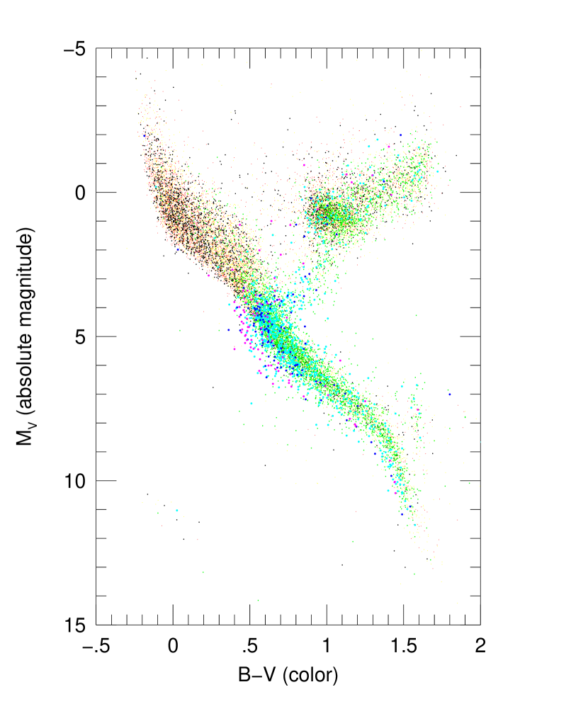
Figure 1: Color-magnitude diagram drawn from the Hipparcos catalog as described in § 2. Black: $v_{\perp}<10\,{\rm km}\,{\rm s}^{-1}$; Red: $10\,{\rm km}\,{\rm s}^{-1}<v_{\perp}<20\,{\rm km}\,{\rm s}^{-1}$; Yellow: $20\,{\rm km}\,{\rm s}^{-1}<v_{\perp}<50\,{\rm km}\,{\rm s}^{-1}$; Green: $50\,{\rm km}\,{\rm s}^{-1}<v_{\perp}<100\,{\rm km}\,{\rm s}^{-1}$; Cyan: $100\,{\rm km}\,{\rm s}^{-1}<v_{\perp}<150\,{\rm km}\,{\rm s}^{-1}$; Blue: $150\,{\rm km}\,{\rm s}^{-1}<v_{\perp}<200\,{\rm km}\,{\rm s}^{-1}$; Magenta: $v_{\perp}>200\,{\rm km}\,{\rm s}^{-1}$.

References

• ESA (1997) European Space Agency (ESA). 1997, The Hipparcos and Tycho Catalogues (SP-1200; Noordwijk: ESA)
Refer to caption