The Tiling Algorithm for the 6dF Galaxy Survey

Abstract

The Six Degree Field Galaxy Survey (6dFGS) is a spectroscopic survey of the southern sky, which aims to provide positions and velocities of galaxies in the nearby Universe. When completed the survey will produce approximately 170000 redshifts and 15000 peculiar velocities. The survey is being carried out on the Anglo Australian Observatory’s (AAO) UK Schmidt telescope, using the 6dF robotic fibre positioner and spectrograph system. We present here the adaptive tiling algorithm developed to place 6dFGS fields on the sky, and allocate targets to those fields. Optimal solutions to survey field placement are generally extremely difficult to find, especially in this era of large-scale galaxy surveys, as the space of available solutions is vast (2N dimensional) and false optimal solutions abound. The 6dFGS algorithm utilises the Metropolis (simulated annealing) method to overcome this problem. By design the algorithm gives uniform completeness independent of local density, so as to result in a highly complete and uniform observed sample. The adaptive tiling achieves a sampling rate of approximately 95%, a variation in the sampling uniformity of less than 5%, and an efficiency in terms of used fibres per field of greater than 90%. We have tested whether the tiling algorithm systematically biases the large-scale structure in the survey by studying the two-point correlation function of mock 6dF volumes. Our analysis shows that the constraints on fibre proximity with 6dF lead to under-estimating galaxy clustering on small scales ($<$1 h^-1 Mpc) by up to $\sim$20%, but that the tiling introduces no significant sampling bias at larger scales. The algorithm should be generally applicable to virtually all tiling problems, and should reach whatever optimal solution is defined by the user’s own merit function.

1 Introduction

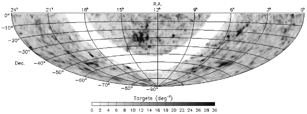
Figure 1: The 6dFGS targets show strong clustering on the sky, as can be seen in this equal–area (Aitoff projection) greyscale map of the surface density of targets. As the 6dF field covers an area of 25.5 deg² and has up to 150 fibres, an optimal surface density would be approximately 6 targets per deg². The large, and spatially complex, density variations about this optimum illustrate one of the major difficulties in tiling the 6dFGS.

The advent of large-scale spectroscopic surveys, made possible by high multiplex spectroscopic systems, has necessitated the development of automated schemes for placing survey fields (‘tiles’) on the sky, and allocating survey targets to those fields. Adaptive tiling schemes take into account survey and instrument characteristics and provide efficient and optimal tile placement and target allocation. The recently completed 2dF Galaxy Redshift Survey (2dFGRS) successfully utilized adaptive tiling to obtain 221414 redshifts, using a 400 fibre spectrograph with a 2^∘ field of view (Colless et al., 2001). The 2dFGRS covered 2000 deg² at a median depth of $\bar{z}=0.11$. The Sloan Digital Sky Survey (SDSS) (York et al., 2000) aims to observe $\sim$10⁶ targets with a 640 fibre system and a 3^∘ field of view, and is also employing adaptive tiling (Blanton et al., 2003). The SDSS will cover $\sim$10000 deg² at a depth similar to the 2dFGRS.

The 6dFGS is a redshift and peculiar velocity survey that will cover the 17000 deg² of the southern sky with $|b|>10$^∘(Watson et al., 2001; Saunders et al., 2001; Wakamatsu et al., 2002). The survey is being carried out on the AAO’s Schmidt telescope, using the 6dF automated fibre positioner and spectrograph system (Parker et al., 1998; Watson et al., 2000). 6dF can simultaneously observe up to 150 targets in a circular 5.7^∘ field of view. Survey observations are made with two different gratings for each field. These two spectral ranges are spliced together as part of the redshifting process, resulting in single spectra that span the range from 3900Å to 7500Å , at a resolution of $R=1000$ at 5500Å and a typical signal-to-noise ratio of $S/N\sim 10$.

The goals of the survey are to map the positions and velocities of galaxies in the nearby Universe, providing new constraints on cosmological models, and a better understanding of the local populations of normal galaxies, radio galaxies, AGN and QSOs (Saunders et al., 2001). The primary targets for the redshift survey are 113988 $K_{s}$-selected galaxies from the 2MASS near-infrared sky survey ((Jarrett et al., 2000); http://www.ipac.caltech.edu/2mass/releases/allsky) down to $K_{tot}<12.75$ and with a median redshift $\bar{z}=0.05$. The total magnitudes are estimated from the 2MASS isophotal $K_{20}$ magnitudes and surface brightness profile information (Jones et al., 2004). Merged with the primary sample are 16 other smaller extragalactic samples, including targets selected from the HIPASS HI radio survey (Koribalski, 2002), the ROSAT All Sky Survey of X-ray sources (Voges et al. (1999, 2000); http://heasarc.gsfc.nasa.gov/docs/rosat/ass.html), the IRAS Faint Source Catalogue ((Moshir et al., 1992); http://irsa.ipac.caltech.edu/IRASdocs/iras.html), the DENIS near-infrared survey (Epchtein et al., 1997), the SuperCosmos $b_{J}$ and $r_{F}$ optical catalogues (Miller et al., 1991), the Hamburg-ESO QSO survey (Wisotzki et al., 2000) and the NVSS radio survey (Condon et al., 1998). In total the survey will produce approximately 170000 redshifts.

The 6dFGS peculiar velocity survey will consist of all early-type galaxies from the primary redshift survey sample that are sufficiently bright to yield precise velocity dispersions. These galaxies are observed at higher signal-to-noise ratio ($S/N>25$), in order to obtain velocity dispersions to an accuracy of 10%. Peculiar velocities will be obtained using the Fundamental Plane for early-type galaxies (Djorgovski & Davis, 1987; Dressler et al., 1987) by combining the velocity dispersions with the 2MASS photometry. Based on the high fraction of early-type galaxies in the $K_{s}$ sample and the $S/N$ obtained in our observations to date, we expect to measure distances and peculiar velocities for 10–15000 galaxies out to distances of at least $cz=15000$ km s^-1.

Observations have so far been made for $40\%$ of the survey fields and completion is expected mid–2005. The data is non-proprietary and an Early Data Release for some 14000 objects can be accessed at http://www-wfau.roe.ac.uk/6dFGS/.

This paper describes the adaptive tiling algorithm developed for the 6dFGS. It is organised in the following manner: §2 outlines the functional requirements for the tiling algorithm and the context in which it was developed; §3 gives a detailed explanation of the algorithm; §4 outlines the process of parameter selection and application of the algorithm to the 6dFGS catalogue; §5 presents an investigation of possible systematic effects introduced by the tiling, and their impact on subsequent analyses of survey data; §6 concludes with a summary of the tiling algorithm and its performance.

Table 1: The distribution of 6dFGS targets in terms of the numbers of neighboring targets within the fibre-button proximity exclusion limit. Only 60% of the catalogue are without close neighbours (as compared with $\sim$90% in the SDSS), meaning a significant proportion have multiple close neighbours, the most extreme being one target with 40 neighbours within 5.71 arcmin.

# Neighbours	# Targets	Sample fraction
0	102252	59.2%
1	43196	25.0%
2	15695	9.1%
$\geq 3$	11604	6.7%

2 Goals and Approach

The fundamental goals of a successful tiling algorithm are completeness, uniformity and efficiency. Given the constraints imposed by the instrument, the tiling algorithm should yield an arrangement of fields that maximizes the fraction of the target sample that is observed (high completeness) with little variation of this fraction with the position or surface density of targets (good uniformity) and with the smallest feasible number of fields (high efficiency).

These goals are particularly challenging for the 6dFGS. The low redshifts of the target samples mean that even in projection on the sky their clustering is strong, with the rms clustering per 6dF field equal to 0.64 of the mean density. Figure 1 shows an equal-area (Aitoff projection) greyscale map of the surface density of targets in the 6dFGS, illustrating the complex variations. There are also significant instrumental constraints on fibre placement due to the large size of the 6dF fibre buttons. These set a lower limit on the proximity of targets that can be allocated to fibres in the same field (see §3.2). There is at least one neighboring target within this proximity limit for 40.8% of the targets in the sample (see Table LABEL:neighbours). Despite these constraints, our requirements for the 6dF tiling algorithm were: (i) completeness, in terms of the fraction of total targets observed, of better than 90%; (ii) uniformity, in terms of the rms variation in randomly-located 6dF fields, to better than 5%; (iii) efficiency, in terms of the average fraction of fibers assigned to targets over all fields, of at least 80%.

The approach adopted in constructing an algorithm to achieve our goals involves a four-stage process: (i) the establishment of a weighting scheme for the target galaxies to account for the relative priorities of the target samples and to allow a balance to be set between completeness and uniformity; (ii) the creation of a proximity exclusion list to account for the instrumental constraint on the closeness with which fibres can be placed; (iii) the initial placement of tiles and allocation of fibres; and (iv) the optimization of the tiling utilizing a Metropolis algorithm (Metropolis et al., 1953), in order to maximize the sum of the weights of all the allocated targets in the tiling.

The Metropolis (simulated annealing) method was adopted because it is effective at searching very complicated parameter spaces and because it is robust against trapping by local, rather than global, maxima (Press et al., 1992). While simulated annealing is expensive in terms of computation time, the entire survey is tiled at once and therefore the annealing need only be performed a few times during the life of the survey, making computation time non-critical.

Note that the tiling algorithm determines the tile locations but does not determine the final allocation of objects to fibres in each tile. This is because the detailed fibre configuration depends on the button and ferrule shape, fibre width, and so on; these have only secondary effect on the overall numbers of configurable targets in a field, and are in any case far too complex and time-consuming to handle within the tiling algorithm. Final allocations are done at the time of observation in a separate step by the 6dF configure software, and also depend on real-time variations in the available fibres on each of the 6dF field plates resulting from breakages and repairs.

The tiling program was initially developed and tested using a synthetic data set. The data came from sets of mock 6dF Galaxy Surveys, constructed from large, high-resolution, N-body cosmological simulations. The 6dF mock volumes have the same radial selection function and geometrical limits as those expected for the real 6dF survey. A full description of the method of generation, and the mock volumes, can be found in Cole et al. 1998. The mock catalogues are publicly available at http://star-www.dur.ac.uk/$\sim$cole/mocks/main.html. Final testing and tuning of the algorithm was done using the 6dFGS target catalogue.

3 Tiling Algorithm

3.1 Weighting Schemes

3.1.1 Density weighting

Our original merit function was simply the overall number of targets configured. However, this leads to a significant bias towards overdense regions. The reason is that for any uniform level of completeness, there are always more unallocated targets per tile in denser regions, so additional tiles will always be placed in denser regions. In effect, the merit function tends to equalise the number of unallocated targets per tile area.

To get around this bias, we investigated the effect of giving each target a weight inversely proportional to the target surface density, when smoothed on tile scales. That is, we gave each target a density weight of

$$D=\left(\frac{n_{6}}{\langle{n_{6}}\rangle}\right)^{\alpha}~{}~{},$$ (1)

where $n_{6}$ is the number of targets within the boundary of a 6dF field centered on the target’s position, $\langle{n_{6}}\rangle$ is the mean number of targets per tile. With a weighting exponent $\alpha$=0 the targets are unweighted, and inverse-density weighted when $\alpha$=-1.

3.1.2 Priority weighting

Beyond the basic goals of high completeness and uniformity, we established a target sample priority scheme to ensure the weighting reflected the relative importance of the various samples in the survey. The priority weight $P$ for a particular target is given by

$$P=\beta^{p}~{}~{},$$ (2)

where $\beta$ is the weighting base and $p$ is the priority value assigned to the target.

The final weight for a target is the product of its density and priority weights, normalised to the total number of targets in the sample.

3.2 Proximity Exclusion

The magnetic buttons of 6dF carry light-collecting prisms attached to optical fibres that feed directly to the spectrograph slit. The buttons are cylindrical and have a 5 mm diameter, equivalent to 5.60 arcmin on the sky. This means that with a 100 $\mu$m safety margin the minimum separation between targets on a single tile is 5.71 arcmin. In optimizing the tiling, it is therefore necessary to have knowledge of each object’s proximity to other targets, in order to prevent the allocation to the same tile of objects closer than the minimum separation.

To achieve this, the entire catalogue of targets is searched, and a list is created containing the number and identification of galaxies that fall within the minimum proximity radius of a given target. This list is consulted whenever fibres are being assigned on a given tile (see §3.3), and if a galaxy within the proximity exclusion zone of the target has already been allocated to that tile, then the target is no longer considered for assignment on that tile. The list is also used to help prioritise the allocation of targets to tiles, as described below.

3.3 Fibre Allocation

Two options were investigated for the initial placement of tiles: a uniform distribution (similar to the 2dFGRS and SDSS tiling algorithms), and placing tiles on random target positions. By doing the latter we gain a headstart in matching the distribution of galaxies on the sky, and tests of both methods showed that this was indeed more computationally efficient for the 6dFGS with its high level of clustering.

The tiling is thus initiated by choosing a target at random, placing a tile centre at that position and assigning targets to that tile. This process is repeated until all the pre-determined number of tiles have been placed, with the proviso that the target chosen at random must not already have been assigned to a tile. This approach allows a uniform random sampling of the galaxy distribution to guide the initial positions of the tiles.

The last step in the initial tiling is a full re-allocation of targets to tiles. For each tile that is to have targets allocated, a list of possible candidates—those within a tile radius of the tile centre, 2.85^∘—is created. Each candidate is given a ranking; those targets with no neighbours within the button proximity exclusion zone (see §3.2) are ranked in order of increasing separation from the tile center, since targets at the edge of the field are more likely to be picked up by overlapping neighbouring fields. Targets with close neighbours are ranked in order of decreasing number of neighbours, and then increasing separation from the tile center. Candidates with close neighbours always rank above candidates without, no matter their separation from the tile center. The latter is to minimize under-sampling of close pairs of targets by giving them higher priority, in order to counteract their preferential loss due to the proximity exclusion constraint. Once the candidate lists are complete, each tile is assigned one target in turn, until each tile has a full complement of targets, or has no more candidates. At all times a target can only be allocated to a tile if it is not already allocated to another tile, and if it is not excluded due to its proximity to a target already allocated to the same tile.

This ‘democratic’ allocation of targets to tiles resulted in higher completeness and less variance in sampling than the initial method we tested, where tiles were ordered by their number of candidates, and the richest tile was allotted a full complement of targets before progressing to the next richest, and so on.

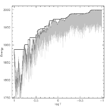
Figure 2: The progress of the tiling algorithm on test data, the horizontal axis showing the control parameter (the ‘temperature’), and the vertical axis the merit function (the ‘energy’). The tiling begins at an energy determined by the initial random allocation of tiles. The tiles are then perturbed and a new configuration is accepted (represented by the dark grey line, with the light grey line showing the rejected configurations). As the temperature decreases the range of changes in the accepted configurations also decreases, as the algorithm refines its search for the optimum tiling. The best configuration at each stage is shown by the heavy black line.

3.4 Optimization Process

The tiling is optimised using the Metropolis algorithm (Metropolis et al., 1953), a method for simulating the natural process of annealing. It uses a control parameter $T$ (by analogy, the ‘temperature’ of the tiling), and an objective function $E$ (the ‘energy’ or merit function of the tiling), whose maximum represents the optimal tiling. The 6dFGS tiling merit function is simply the sum of the weighted values of all the allocated targets of a tiling.

The annealing process is an iterative one which begins at some predetermined temperature and at an initial value for the merit function $E_{1}$ computed from the initial placement of tiles and allocation of targets (see §3.3). We then need some way to perturb the position of one or more tiles. This step was the subject of extensive investigation. Early versions perturbed the positions of all tiles simultaneously. However, this was found to be grossly inefficient, because almost all such global perturbations are unfavourable as a solution is approached. We therefore switched to perturbing a small subset of the tiles. It was found that to randomly select and arbitrarily reposition a single tile was also inefficient, because virtually all such individual repositionings are unfavourable. Therefore, the tile movement was selected from a 2D Gaussian, with rms 10% of the tile width in each of RA and Dec. This increased run speed to give feasible timescales, but the tiling configuration tended to get stuck in local maxima, where no individual tile adjustment improved the yield. A change was then made so that in 50% of cases, all tiles within a radius of 3 tile diameters of the randomly selected tile were perturbed together, with the perturbation falling off as a Gaussian with scale length 1 tile diameter. This gave both acceptable run times and acceptable solutions.

Following a pertubation, all nearby tiles (defined as tiles within the circle of influence of the perturbation, with a safety margin of a degree) then have targets reallocated. Reallocation for all tiles was neither necessary nor computationally feasible. After this re-allocation the merit function of the new tiling $E_{2}$ is computed, and it is adopted as the current tiling with probability

$$P(E_{2}|E_{1})=\Bigg{\{}\begin{array}[]{cr}1&E_{2}\geq E_{1}\\ &\\ exp\left[(E_{2}-E_{1})/T\right]&E_{2}<E_{1}.\end{array}$$ (3)

Hence, more successful (higher energy) tilings are always accepted, while the chances of a less successful (lower energy) tiling being accepted decrease exponentially with the difference in the merit function, scaled by the temperature.

After each iteration the temperature is decreased, meaning the probability of accepting a tiling with a lower energy than the previous one decreases as the annealing progresses. The possibly large backward steps acceptable at the initial stages of the process are replaced by finer changes as the tiling approaches its optimal configuration (see Fig.2). This continues until some predetermined final temperature, or all the targets have been allocated, whichever comes first. The final tiling is the highest-energy tiling that occurs during the whole course of the optimisation process.

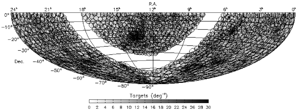
Figure 3: By superimposing the fields from a tiling on the target surface density map, we can see how the tiling algorithm results in a proportional coverage in terms of surface density, and yet still provides complete coverage of the survey volume. Hence the adaptive tiling can achieve high completeness, as well as highly uniform completeness.

4 Application of the Algorithm

Initial survey observations were begun in a strip of the sky covering 0–360^∘R.A. and -23^∘to -42^∘in Dec., the first of the three strips of the sky selected in the survey observing strategy. These observations were made without the aid of a tiling algorithm and based on a provisional catalogue. Upon completion of the algorithm the strip was tiled, with the 50 fields already observed being included in the tiling as fixed fields. The entire survey was then tiled with the completion of the full catalogue. The algorithm parameter values used had been refined through testing upon the mock volumes and the initial Dec. strip. The tiling will continue to be an ongoing process during the life of the survey in order to accommodate changes in strategy or circumstance. Such a circumstance arose when it became apparent in the second year of operations that inefficiencies, particularly in the early stages of the survey, required a retiling with revised tile and fibre numbers.

Table 2: The completeness levels for various weighting schemes using different maximum fibre numbers per 6dF tile. The $\alpha$-value represents the weighting exponent for the surface density weighting , with $\alpha=0$ corresponding to uniform weights, and $\alpha=-1$ corresponding to proportional weights (see §3.1.1). The $\beta$-value is the base for the priority weighting, with $\beta=1$ meaning no priority weighting, and $\beta=2$ meaning a difference of +1 in priority makes a target twice as likely to be selected (see §3.1.2). The fibre numbers were based on what we could reasonably expect to be able to use on average, taking into account mechanical constraints and attrition.

Weighting	Priority	Completeness
scheme		125 fibres	130 fibres	135 fibres
	8	94.0%	95.1%	95.1%
$\alpha=0$	6	95.8%	97.1%	97.1%
$\beta=1$	5	86.7%	88.1%	89.0%
	4	97.2%	98.3%	98.8%
Total		94.5%	95.6%	95.7%
	8	94.9%	95.6%	95.9%
$\alpha=0$	6	93.3%	94.8%	95.8%
$\beta=2$	5	83.8%	83.0%	85.1%
	4	93.7%	96.4%	96.7%
Total		94.1%	95.1%	95.7%
	8	91.2%	92.5%	94.3%
$\alpha=-1$	6	93.9%	94.6%	96.3%
$\beta=1$	5	87.8%	88.4%	89.3%
	4	97.5%	97.6%	98.4%
Total		92.2%	93.3%	94.9%
	8	92.6%	93.8%	94.7%
$\alpha=-1$	6	91.5%	93.3%	94.3%
$\beta=2$	5	85.2%	84.4%	84.6%
	4	95.3%	95.6%	95.7%
Total		92.3%	93.6%	94.4%

4.1 Tile and Fibre Numbers

We attempted to predict a reasonable number of fibres which could be configured per field, given the high target clustering and mechanical constraints such as fibre breakages and fibre crossings. Of the 150 fibres nominally available, 10 are normally assigned to blank sky positions, leaving 140 for survey targets. Instrument commissioning and the initial stages of the survey suggested we could expect to be able to configure 135 of these 140 fibres per field. We compared tiling results for a range of available fibres per tile (see Table LABEL:fibres), and decided to limit fibre numbers within the algorithm to 135 per tile. Based on this we needed $\sim 1330$ tiles to match target numbers. The numbers of targets with neighbours within the fibre button proximity exclusion zone (see Table LABEL:neighbours) also indicated we needed to oversample the sky at least 1.5 times. Choosing 2 x oversampling, which equated to 1360 tiles, gave us the best balance between potential sample completeness and achievable tile numbers given the expected life-time of the survey. The first full tiling of the catalogue was therefore tiled with 1360 tiles, each of which could be allocated a maximum of 135 targets.

By the beginning of the second year of the survey, however, it had become apparent that this number of allocations was unrealisable, primarily due to a higher than expected attrition rate of fibres. We therefore revised the maximum available number of fibres downwards to 125 per tile, and accordingly increased the total number of tiles to 1564 (1000 tiles for the revised tiling, and 564 tiles from the original tiling which had been observed).

4.2 Annealing Schedule

The annealing schedule, by which is meant the initial and final temperatures and the steps between them, had to be chosen as a compromise between efficacy and speed. The initial temperature determines the size and frequency of negative changes to the tiling configuration. Too large an initial temperature and tiles would be relocated outside the survey region and be unable to return. Too low an initial temperature and the annealing was unable to break out of locally maximal configurations to achieve the global optimum. The minimum temperature needed to be sufficiently small to allow the annealing to perform to our expectations, without proving impractical in terms of computation time. Finally, the temperature scale (the amount by which the temperature is decreased after each iteration of the annealing) needed to quench the tiling slowly enough to allow the annealing to perform, but again could not be so slow that it would be computationally infeasible. After testing, an initial temperature of 10 and a final temperature of 0.1 were settled on. The temperature scale was chosen to be a maximum of 1% of the current temperature of the annealing, scaled inversely to the number of tiles being configured. The larger the tiling, the smaller the temperature scale, ensuring the annealing is quenched more slowly in proportion to the complexity of the parameter space.

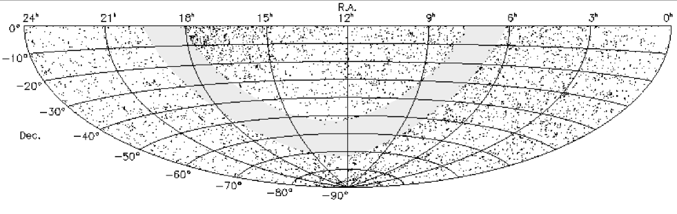
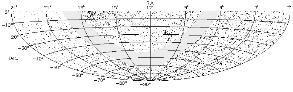
Figure 4: The distribution of the survey targets not allocated to tiles, in tilings using uniform (top) and proportional (bottom) density weights. The almost uniformly random distribution is evidence of the success of the tiling in sampling in a highly uniform fashion. The increased uniformity of the proportional weighting relative to the uniform weighting is seen in the decrease in ‘holes’ (regions of high target density where all targets have been allocated) in the distribution, and particularly in the better performance along the edges of the survey.

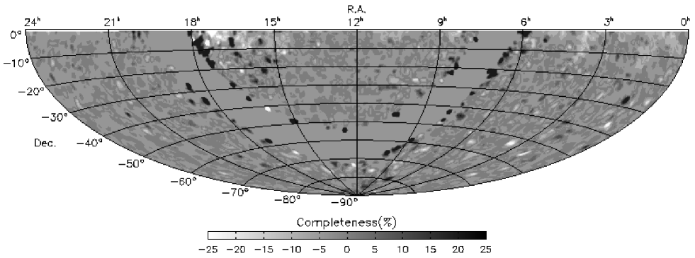
Figure 5: A difference map of the completeness between the uniform and proportional tilings of the survey: a positive difference in favour of the proportional tiling is shown in darker colours, while a negative difference is shown in lighter colours. The improved performance of the proportional tiling along the edges of the survey are obvious.

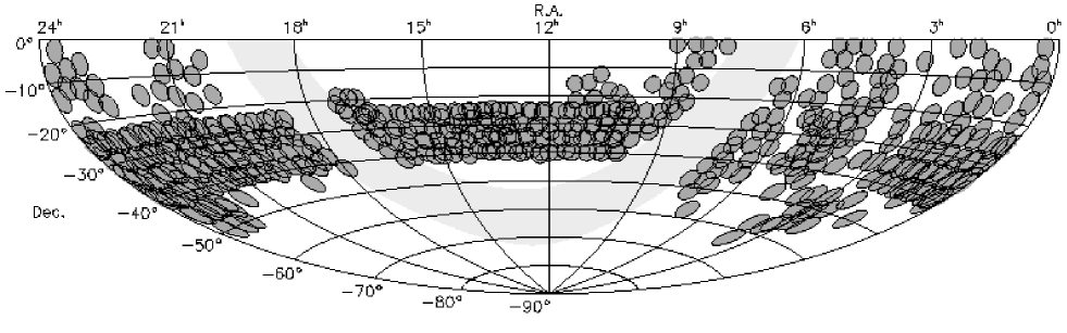
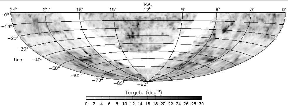
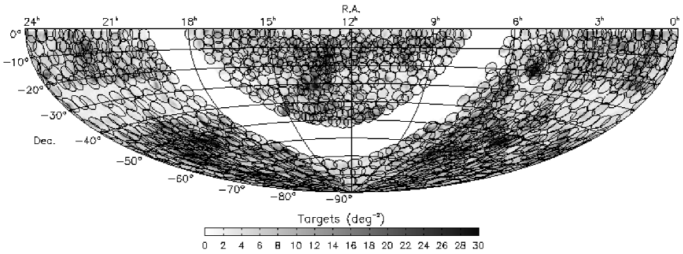
Figure 6: When it became necessary to retile the survey, 564 fields from the original tiling had already been observed (top), most within the central declination strip of the survey ($-$23^∘ to $-$42^∘). The targets observed successfully within those fields were re-prioritized so as not to be included in the new tiling, resulting in a very different distribution to be tiled (middle). The algorithm again provided a tiling solution matched to the target distribution (bottom) which resulted in a highly complete and efficient sampling of the survey targets.

Table 3: Performance statistics for the tilings of the 6dFGS catalogue, concentrating on the three fundamental criteria of completeness, efficiency, and uniformity (given by the rms variation in completeness). The survey was tiled using both a uniform ($\alpha=0$) and a proportional ($\alpha=-1$) weighting scheme. Both tilings exceeded the performance requirements set for the algorithm.

Weighting	Completeness				Efficiency
	Mean	Median	Total	RMS	Mean	Median	RMS
${\alpha=0}$	94.0%	96.0%	95.2%	3.8%	87.3%	90.4%	11.5%
${\alpha=-1}$	94.5%	95.8%	94.9%	3.3%	87.0%	91.8%	13.3%

Table 4: Completeness results for individual target samples in order of observational priority. All the tilings provide excellent completeness, with only a small number of lower-priority samples falling below 90%, due to the fibre button proximity exclusion. The highest priority targets are consistently at $\sim$95%, indicating the success of the priority weighting scheme.

Sample	ID	Priority	Targets	Completeness
				${\alpha=0}$	${\alpha=-1}$
2MASS K${}_{s}<12.75$	1	8	113988	95.9%	95.7%
2MASS H$<13.05$	3	6	3282	93.7%	94.0%
2MASS J$<13.75$	4	6	2008	94.5%	94.3%
Supercosmos $r_{F}<15.7$	7	6	9199	95.8%	95.4%
Supercosmos $b_{J}<17.0$	8	6	9749	96.7%	96.5%
Shapley	90	6	939	98.7%	98.2%
ROSAT All-Sky Survey	113	6	2913	95.7%	95.4%
HIPASS $(>4\sigma)$	119	6	821	87.7%	85.8%
IRAS Faint Source Catalogue	126	6	10707	96.3%	95.7%
Denis J$<14$	5	5	1505	91.9%	91.5%
Denis I$<15$	6	5	2017	74.3%	73.9%
2MASS AGN	116	4	2132	95.7%	95.9%
Hamburg-ESO Survey	129	4	3539	96.7%	96.9%
NOAO-VLA Sky Survey	130	4	4334	96.3%	96.7%

4.3 Weighting Schemes

All of the targets in the 6dFGS catalogue have a priority based on the relative observational importance of their particular survey sample. The primary target sample has the highest priority of 8, while other samples were ranked in order of their completeness requirements (lower numbers are lower priority). Targets must have a minimum priority of 4 to be considered in the tiling. All targets which require only serendipitous coverage, and all successfully observed targets have priorities less than this minimum; such targets may be included in an actual fibre configuration (with low priority) but do not influence the tiling of the survey (recall that the final allocation of fibres to targets is done in a separate step at the time of observation; see §2).

The priority weighting scheme uses a weighting base $\beta=2$, so that a target with a priority one higher than another target should be twice as likely to be allocated, based solely on its priority weight. Comparisons of tilings with and without priority weighting typically showed an increase in the completeness of the primary target sample (priority 8) of up to 1%, with lower-priority samples showing decreases of between 2% and 5% (Table LABEL:fibres).

When tiling the 6dFGS catalogue, the quantity $n_{6}$ in the density weighting (see §3.1.1) is calculated from the number of targets in the 2MASS $K_{s}$-selected sample alone, since this is the primary homogeneous all-sky sample. There were two ‘natural’ values of the density weighting exponent $\alpha$ we could use, 0 and $-$1, which we term uniform and proportional weighting respectively. We want completeness, a fractional measure, to be high and uniform, but the simplest algorithm ($\alpha=0$) just optimises on number, an absolute measure. If we weight uniformly, then the gain for a new tile goes like $\Delta n$ (the number of new targets acquired), which tends to maximise overall completeness; if we weight inversely by local density ($\alpha=-1$), then we gain as $\Delta n/n_{6}$, which maximizes local completeness, and so improves uniformity. In other words, uniform density weighting optimizes global completeness, while proportional density weighting optimizes local completeness, and hence both completeness and uniformity. The 6dFGS catalogue can always be used to accurately determine the true sampling as a function of position, provided the sampling of the catalogue is not biased in terms of spectroscopic or photometric properties of the targets. This variable sample can then be accounted for in subsequent analyses (Colless et al., 2001). However, highly uniform sampling keeps such corrections to a minimum; we therefore preferred, a priori, the proportional density weighting.

4.4 Performance analysis

The tilings surpassed all of the goals of completeness, uniformity, and efficiency set for the algorithm (see Table LABEL:stats). The tiling optimization had the desired effect of increasing tile numbers in over-dense regions, while still providing uniform sampling of the sky and sample (see Figure 3). The algorithm also proved to be very flexible, able to handle the highly irregular survey volume it was presented with in the revised tiling (see Figure 6).

As expected, the uniform weighting scheme resulted in the highest overall completeness (since the tiling preferred the target-rich densely-clustered regions), but resulted in less-uniform sampling than the proportional weighting. As a simple form of analysis, if we display those targets that were not allocated to fibres in the tilings, they should appear to be uniformly randomly distributed across the sky. Figure 4 shows this is the case, however the uniform tiling does show a relatively less uniform distribution, in particular empty regions and concentrations of targets along the edges of the survey. This edge effect is highly apparent in Figure 5 which shows a map of the difference in completeness between the two tilings. The dark regions show areas where the proportional tiling resulted in higher sampling, while the lighter shows superior performance by the uniform tiling. An edge-avoidance effect is an understandable result of uniform tiling, since fields placed close to the edges effectively have lower density and hence fewer available targets. The proportional tiling’s ability to reduce this edge effect is another facet of its improved uniformity of sampling.

Table LABEL:samples shows the completeness levels for individual target samples. The results are excellent, with only Denis I and HIPASS sources falling below 90%. Denis I targets were missed due to high surface densities, the result of stellar contamination near the Galactic Plane. The HIPASS result can be explained by the fact that these targets are being used to confirm the optical counterparts to radio sources, where there are multiple possibilities in close proximity to each other. Therefore these two samples suffer the most from the button proximity constraint.

Close inspection of Figure 4 does show small concentrations of unallocated targets, and indications of two regions of relatively poorer sampling for both tilings. The small concentrations of unallocated targets are primarily Denis I targets mentioned above. The North Galactic equatorial region between $15^{h}$ and $18^{h}$ and the South Galactic Pole however, suffer due to the combination of their low surface densities and their proximity to the Galactic Equator. Firstly, their low surface densities mean the initial random allocation of tiles will sample these areas more sparsely. Secondly, tiles are unlikely to migrate through the Equator, and hence it acts as a barrier to the free movement of the tiles. A remedy for this would of course be to increase tile numbers, however given the success of the tiling and the small gains to be had, along with the constraint of a limited survey lifetime, this was not deemed necessary.

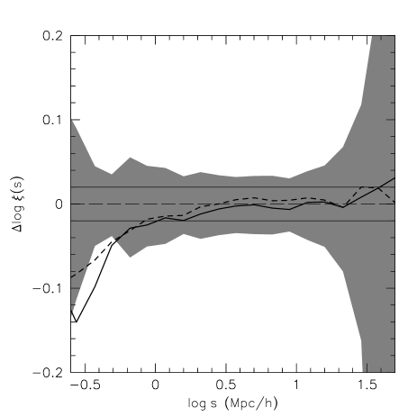
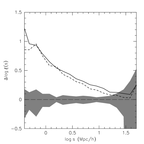
Figure 7: A comparison of the mean difference in the logs of the recovered $\xi(s)$ and the true value of $\xi(s)$, based on the allocated (top) and unallocated (bottom) targets from tiling 10 6dF mock volumes. The solid line represents the results from proportional tilings, while the dashed line represents uniform tilings. The shaded region is the $\pm 1\sigma$ variation about the mean $\xi(s)$. The solid line either side of the zero line represents a 5% difference from the mean $\xi(s)$. While the recovered correlations are consistent with the true values at large scales, there is obvious under-estimation at smaller scales equivalent to the size of a 6dF fibre button.

5 Systematic Effects

In order to determine the nature of any sampling biases introduced by the tiling algorithm, and quantify their systematic effects, we compared the two-point correlation functions of the objects in the tiled and full samples based on mock 6dF catalogues.

We computed the correlation functions using the Landy and Szalay estimator (Landy & Szalay, 1993). One change was made to accommodate the wide angular coverage of the 6dFGS. The redshift space separation between two nearby galaxies is given by

$$s=\sqrt{s_{1}^{2}+s_{2}^{2}-2s_{1}s_{2}cos\theta}$$ (4)

where $s_{1}$ and $s_{2}$ are the redshift space distances of the galaxies, and $\theta$ is their angular separation on the sky. However, this Euclidean approximation is insufficient for such a wide-angle survey as the 6dFGS. The general formula developed by Matsubara (2000), which includes wide-angle effects and cosmological distortions, reduces, in the case of a flat Universe, to

$$d=\sqrt{d_{1}^{2}+d_{2}^{2}-2d_{1}d_{2}cos\theta}$$ (5)

where $d$ is the co-moving distance of a galaxy.

The correlation function code was applied to a number of 6dF mock volumes, and the results were consistent both with the known correlation function of the mocks and the observed correlation functions from the 2dFGRS (Hawkins et al., 2002) and SDSS (Zehavi et al., 2002) surveys. Once we had established the correlation code was working satisfactorily, we were able to test for bias by applying it to the galaxies in 10 mock 6dF Galaxy Surveys, and to the allocated and unallocated targets resulting from applying the tiling algorithm to these mock surveys. Bias would most likely appear in two forms:

1. The tiled sample might over- or under-represent clustered regions of galaxies. This would distort $\xi(s)$ on the scale of a 6dF tile, that is $\sim$6^∘, corresponding to $\sim$20 h^-1 Mpc  at the median redshift of the survey ($z\approx 0.05$).

2. The fibre proximity exclusion constraint might result in the loss of close pairs of galaxies, distorting $\xi(s)$ on small scales. The button size of 5 arcmin corresponds to $\sim$0.3 h^-1 Mpc  at $z\approx 0.05$.

Figure 7 shows a comparison of the mean difference in the logs of the recovered $\xi(s)$ and the true value of $\xi(s)$, for both proportional (solid line) and uniform (dashed line) tilings. The shaded region is the $\pm 1\sigma$ variation about the mean $\xi(s)$ for the 10 mock surveys. The solid line either side of the zero line represents a 5% difference from the mean $\xi(s)$. Both proportional and uniform tilings produce estimates of $\xi(s)$ equivalent to the true value, within the errors, at scales larger than about 1 h^-1 Mpc. Even the correlation for the unallocated targets, which exaggerates the effect of any bias, is unaffected at scales equal to a 6dF tile and larger. This suggests no significant sampling bias is occurring due to under or over-representation of clustered regions of galaxies. At small scales however the effects of the button proximity exclusion are readily apparent. At $\sim$0.3 h^-1 Mpc, the scale corresponding to a 6dF fibre button, $\xi(s)$ is under-estimated by $\sim$20%. This sampling bias at small scales must therefore be taken into account in analysis of 6dFGS data.

6 Conclusion

Utilizing an optimization method based on simulated annealing, we have successfully developed an adaptive tiling algorithm to optimally place 6dFGS fields on the sky, and allocate targets to those fields. The algorithm involves a four-stage process: (i) establishing individual target weights based on target surface density and sample observational priorities; (ii) creating a database of all possible conflicts in allocating neighbouring targets closer than the radius of a 6dF fibre button; (iii) creating an initial tiling by centering tiles on randomly selected targets, and then allocating targets to those tiles in order of decreasing numbers of neighbours and increasing separation from tile centres; (iv) and finally, using the Metropolis method in randomly shifting the position of tiles, and then reallocating targets, to maximise the objective function of the tiling and hence provide an optimal tiling solution.

In order to maximise the uniformity of sampling of the 6dFGS targets, we weight inversely with the surface density of 2MASS $K_{s}$ galaxies. Our results showed this gave us superior uniformity when compared with a simple uniform density weighting scheme, most noticeably in reducing the number of targets not allocated to tiles along the edges of the survey volume.

Despite the challenges of highly clustered targets and large fibre buttons, tiling solutions generated using the algorithm are highly complete and uniform, and employ an efficient use of tiles. The tilings consistently give sampling rates of around 95%, with variations in the uniformity of sampling of less than 5%. Tiles typically have more than 90% of their available fibres allocated to targets. The algorithm has also proved itself highly flexible, able to perform on highly irregularly shaped distributions of targets.

An analysis of the two-point correlation function, calculated from 6dF mock volumes tiled with the algorithm, revealed that the constraint on fibre proximity due to the large size of the fibre buttons produces a significant under-sampling of close pairs of galaxies on scales of 1  h^-1 Mpc and smaller; on larger scales, however, the tiling algorithm does not lead to any detectable sampling bias.

References

- Blanton et al. (2003) Blanton M. R., Lin H., Lupton R. H., Maley F. M., Young N., Zehavi I., Loveday J., 2003, AJ, 125, 2276
- Cole et al. (1998) Cole S., Hatton S., Weinberg D. H., Frenk C. S., 1998, MNRAS, 300, 945
- Colless et al. (2001) Colless M., Dalton G., Maddox S., et al., 2001, MNRAS
- Condon et al. (1998) Condon J. J., Cotton W. D., Greisen E. W., Yin Q. F., Perley R. A., Taylor G. B., Broderick J. J., 1998, AJ, 115, 1693
- Djorgovski & Davis (1987) Djorgovski S., Davis M., 1987, ApJ, 313, 59
- Dressler et al. (1987) Dressler A., Lynden-Bell D., Burstein D., Davies R. L., Faber S. M., Terlevich R., Wegner G., 1987, ApJ, 313, 42
- Epchtein et al. (1997) Epchtein N., de Batz B., Capoani L. e. a., 1997, The Messenger, 87, 27
- Hawkins et al. (2002) Hawkins E., Maddox S., Cole S., Madgwick D., Norberg P., Peacock J., Baldry I., Baugh C. e. a., 2002, astro-ph/0212375, pp 12375–+
- Jarrett et al. (2000) Jarrett T. H., Chester T., Cutri R., Schneider S., Skrutskie M., Huchra J. P., 2000, AJ, 119, 2498
- Jones et al. (2004) Jones H., Saunders W., Colless M., Read M., Watson F., Campbell L., Burkey D., Hartley M., 2004, In preparation
- Koribalski (2002) Koribalski B. S., 2002, in Seeing Through the Dust, ASP Conf. Series, The HI Parkes All-Sky Survey (HIPASS)
- Landy & Szalay (1993) Landy S. D., Szalay A. S., 1993, ApJ, 412, 64
- Matsubara (2000) Matsubara T., 2000, ApJ, 535, 1
- Metropolis et al. (1953) Metropolis N., Rosenbluth A. W., Rosenbluth M. N., Teller A. H., Teller E., 1953, J.Chem. Phys., 21
- Miller et al. (1991) Miller L., Cormack W., Paterson M., Beard S., Lawrence L., 1991, in eds. H.T. MacGillivray Thomson E., eds, , Digitised Optical Sky Surveys. Kluwer Academic Publishers, p. 133
- Moshir et al. (1992) Moshir M., Kopman G., Conrow T. A. O., 1992, IRAS Faint Source Survey, Explanatory supplement version 2. Pasadena: Infrared Processing and Analysis Center, California Institute of Technology, 1992, edited by Moshir, M.; Kopman, G.; Conrow, T. a.o.
- Parker et al. (1998) Parker Q. A., Watson F. G., Miziarski S., 1998, in ASP Conf. Ser. 152: Fiber Optics in Astronomy III 6dF: an Automated Multi-Object Fiber Spectroscopy System for the UKST. pp 80+
- Press et al. (1992) Press W. H., Teukolsky S. A., Vetterling W. T., Flannery B. P., 1992, Numerical Recipes in Fortran. Cambridge University Press
- Saunders et al. (2001) Saunders W., Parker Q., Watson F., Frost G., Farrell T., Gillingham P., Hingley B., Muller R., Stevenson J., McCowage C., Colless M., 2001, AAO Epping Newsletter, 97, 14
- Voges et al. (1999) Voges W., Aschenbach B., Boller T., Brauninger H., Briel U., Burkert W., Dennerl K., Englhauser J. e. a., 1999, AAP, 349, 389
- Voges et al. (2000) Voges W., Aschenbach B., Boller T., Brauninger H., Briel U., Burkert W., Dennerl K., Englhauser J. e. a., 2000, in IAU Circular, Rosat All-Sky Survey Faint Source Catalogue. pp 3–+
- Wakamatsu et al. (2002) Wakamatsu K., Colless M., Jarrett T., Parker Q. A., Saunders W., Watson F. G., 2002, in IAU Regional Assembly, ASP Conf. Proc., in press, The 6dF Galaxy Survey
- Watson et al. (2001) Watson F. G., Bogatu G., Saunders W., Farrell T. J., Russel K. S., Hingley B. E., Miziarski S., Gillingham P. R., 2001, in ASP Conference Series All-sky spectroscopic surveys and 6df
- Watson et al. (2000) Watson F. G., Parker Q. A., Bogatu G., Farrell T. J., Hingley B. E., Miziarski S., 2000, in Proc. SPIE Vol. 4008, p. 123-128, Optical and IR Telescope Instrumentation and Detectors, Masanori Iye; Alan F. Moorwood; Eds. Vol. 4008, Progress with 6dF: a multi-object spectroscopy system for all-sky surveys. pp 123–128
- Wisotzki et al. (2000) Wisotzki L., Christlieb N., Bade N., Beckmann V., Köhler T., Vanelle C., Reimers D., 2000, A&A, 358, 77
- York et al. (2000) York D. G., Adelman J., Anderson J. E., et al., 2000, AJ, 120, 1579
- Zehavi et al. (2002) Zehavi I., Blanton M. R., Frieman J. A., Weinberg D. H., Mo H. J., Strauss M. A., Anderson S. F., Annis J. e. a., 2002, ApJ, 571, 172