The 6dF Galaxy Survey: Samples, Observational Techniques and the First Data Release

Abstract

The 6dF Galaxy Survey (6dFGS) aims to measure the redshifts of around 150 000 galaxies, and the peculiar velocities of a 15 000-member sub-sample, over almost the entire southern sky. When complete, it will be the largest redshift survey of the nearby universe, reaching out to about $z\sim 0.15$, and more than an order of magnitude larger than any peculiar velocity survey to date. The targets are all galaxies brighter than $K_{\rm tot}=12.75$ in the 2MASS Extended Source Catalog (XSC), supplemented by 2MASS and SuperCOSMOS galaxies that complete the sample to limits of $(H,J,r_{F},b_{J})=(13.05,13.75,15.6,16.75)$. Central to the survey is the Six-Degree Field (6dF) multi-fibre spectrograph, an instrument able to record 150 simultaneous spectra over the $5.7^{\circ}$-field of the UK Schmidt Telescope. An adaptive tiling algorithm has been employed to ensure around 95% fibering completeness over the 17046 deg² of the southern sky with $|\,b\,|>10^{\circ}$. Spectra are obtained in two observations using separate V and R gratings, that together give $R\sim 1000$ over at least 4000 – 7500 Å and signal-to-noise ratio $\sim 10$ per pixel. Redshift measurements are obtained semi-automatically, and are assigned a quality value based on visual inspection. The 6dFGS database is available at http://www-wfau.roe.ac.uk/6dFGS/, with public data releases occuring after the completion of each third of the survey.

1 INTRODUCTION

Wide-scale redshift surveys such as the 2dF Galaxy Redshift Survey and Sloan Digital Sky Survey (2dFGRS, Colless et al. 2001b; SDSS, York et al. 2001) have made significant advances in our understanding of the matter and structure of the wider universe. These include the precise determination of the luminosity function of galaxies (e.g. Folkes et al. 1999, Cross et al. 2001, Cole et al. 2001, Blanton et al. 2001, Madgwick et al. 2002, Norberg et al. 2002, Blanton et al. 2003), the space density of nearby rich galaxy clusters (De Propris et al. 2002, Goto et al. 2003), and large-scale structure formation and mass density (Peacock et al. 2001, Percival et al. 2001, Efstathiou et al. 2002, Verde et al. 2002, Lahav et al. 2002, Zehavi et al. 2002, Hawkins et al. 2003, Szalay et al. 2003).

While such surveys have also greatly refined our view of the local universe, better determination of several key parameters can be made where a knowledge of galaxy mass can be combined with redshift. The 2dFGRS and SDSS surveys are both optically-selected, inevitably biasing them in favour of currently star-forming galaxies. The 2dF and Sloan spectrographs also have fields of view too small to allow full sky coverage in realistic timescales, limiting their utility for dynamical and cosmographic studies. The 6dF Galaxy Survey (6dFGS) is a dual redshift/peculiar velocity survey that endeavours to overcome the limitations of the 2dFGRS and SDSS surveys in these areas.

The primary sample for the 6dFGS is selected in the $K_{s}$ band from the 2MASS survey (Jarrett et al. 2000). The magnitudes used in the selection are estimated total magnitudes. These features combined mean that the primary sample is as unbiased a picture of the universe, in terms of the old stellar content of galaxies, as is possible at the current time. The near-infrared selection also enables the survey to probe closer to the Galactic equator before extinction becomes an issue; the survey covers the entire southern sky with $|\,b\,|>10^{\circ}$.

The redshift of a galaxy includes both recessional and peculiar velocity components, so that a redshift survey alone does not furnish a true three-dimensional distribution for the galaxies. However, by measuring these components separately, it is possible to determine the three-dimensional distributions of both the galaxies and the underlying mass.

Observationally, significantly greater effort is required to obtain the distances and peculiar velocities of galaxies than their redshifts. Distance estimators based on the Fundamental Plane of early-type galaxies (FP; Dressler et al. 1987, Djorgovski & Davis 1987), as used in the 6dFGS, require measurements of the galaxies’ internal velocity dispersions. Velocity dispersions demand a signal-to-noise ratio (S/N) in the spectrum at least 3 to 5 times higher than redshift measurements. Furthermore, the FP distance estimators need such spectroscopy to be supported by photometry which can be used to determine the galaxies’ surface brightness profiles.

We measure peculiar velocities as the discrepancy between the redshift and the estimated distance. For realistic cosmologies, peculiar velocities increase weakly with distance, but remain $<1000\mbox{\,km\,s${}^{-1}$}$. Redshift errors are small, and have little or no dependence on distance. On the other hand, all existing distance estimators have significant, intrinsic and fractional, uncertainties in distance; for the FP estimators this uncertainty is typically about 20% for a single galaxy measurement. This linear increase in the errors with distance, compared with more or less fixed peculiar velocities, means that the uncertainty on a single peculiar velocity becomes dominated by the intrinsic uncertainties at redshifts $cz\sim 5000\mbox{\,km\,s${}^{-1}$}$. Consequently, all previous peculiar velocity surveys have traced the velocity field, and hence the mass distribution, only out to distances of about 5000 km s^-1 (for relatively dense field samples of individual galaxies; e.g. Dressler et al. 1987, Giovanelli et al. 1998, da Costa et al. 2000) or 15000 km s^-1 (for relatively sparse cluster samples, where distances for multiple galaxies are combined; e.g. Lauer and Postman 1994, Hudson et al. 1999, Colless et al. 2001a). The smaller volumes are highly subject to cosmic variance, while the larger volumes are too sparsely sampled to reveal much information about the velocity field. In order to differentiate cosmological models, and constrain their parameters, both the survey volume and galaxy sampling need to be significantly increased. Moreover, since peculiar velocities amount to at most a few per cent of the velocity over much of the volume, both the underlying sample and the direct distance estimates have to be extraordinarily homogeneous, preferably involving unchanging telescopes, instrumental set ups and procedures in each case.

The two facets of the 6dF Galaxy Survey are a redshift survey of 150 000 galaxies over the southern sky, and a peculiar velocity survey of a subset of some 15 000 of these galaxies.

The aims of the redshift survey are: (1) To take a near-infrared selected sample of galaxies and determine their luminosity function as a function of environment and galaxy type. From these, the stellar mass function and mean stellar fraction of the local universe can be ascertained and compared to the integrated stellar mass inferred from measures of cosmic star formation history. (2) To measure galaxy clustering on both small and large scales and its relation to stellar mass. In doing so, the 6dFGS will provide new insight into the scale-dependence of galaxy biasing and its relationship to dark matter. (3) To determine the power spectrum of this galaxy clustering on scales similar to those spanned by the 2dF Galaxy Redshift Survey and Sloan Digital Sky Surveys. (4) To delineate the distribution of galaxies in the nearby universe. The 6dFGS will not cover as many galaxies as either the 2dF Galaxy Redshift Survey or Sloan Digital Sky Survey. However, because it is a large-volume survey of nearby galaxies, it provides the ideal sample on which to base a peculiar velocity survey. In this respect, the complete 6dFGS will be more than ten times larger in number and span twice the volume of the PSCz Survey (Saunders et al. 2000), previously the largest survey of the local universe. (5) To furnish a complete redshift catalogue for future studies in this regime. As discussed above, precise distance measures impose stronger demands on signal-to-noise than do redshifts. With such higher quality spectra, it is also possible to infer properties of the underlying stellar population, such as ages and chemical abundances. Having such measurements along with the galaxy mass and knowledge of its local envrionment, will afford unprecedented opportunities to understand the processes driving galaxy formation and evolution.

This redshift catalogue will provide the basis for a volume-limited sample of early-type galaxies for the peculiar velocity survey. The aims of the peculiar velocity survey are: (1) A detailed mapping of the density and peculiar velocity fields to around 15000 km s^-1  over half the local volume. (2) The inference of the ages, metallicities and star-formation histories of E/S0 galaxies from the most massive systems down to dwarf galaxies. The influence of local galaxy density on these parameters will also be of key interest to models of galaxy formation. (3) To understand the bias of galaxies (number density versus total mass density field) and its variation with galaxy parameters and environment.

One novel feature of the 6dF Galaxy Survey compared to earlier redshift and peculiar velocity surveys is its near-infrared source selection. The main target catalogues are selected from the Two Micron All Sky Survey (2MASS; Jarrett et al. 2000) using total galaxy magnitudes in $JHK$. There are several advantages of choosing galaxies in these bands. First, the near-infrared spectral energy distributions (SEDs) of galaxies are dominated by the light of their oldest stellar populations, and hence, the bulk of their stellar mass. Traditionally, surveys have selected target galaxies in the optical where galaxy SEDs are dominated by younger, bluer stars. Second, the E/S0 galaxies that will provide the best targets for Fundamental Plane peculiar velocity measures represent the largest fraction by galaxy type of near-infrared-selected samples. Finally, the effects of dust extinction are minimal at long wavelengths. In the target galaxies, this means that the total near-infrared luminosity is not dependent on galaxy orientation and so provides a reliable measure of galaxy mass. In our own Galaxy, it means the 6dFGS can map the local universe nearer to the plane of the Milky Way than would otherwise be possible through optical selection.

In this paper we describe the key components contributing to the realisation of the 6dF Galaxy Survey. Section 2 describes the Six-Degree Field instrument; section 3 details the compilation of the input catalogues and the optimal placement of fields and fibres on sources therein; section 4 outlines the methods used to obtain and reduce the spectra, and derive redshifts from them; section 5 summarises the First Data Release of 46 474 unique galaxy redshifts and describes the 6dF Galaxy Survey on-line database; section 6 provides concluding remarks.

2 THE SIX-DEGREE FIELD SPECTROGRAPH

Central to the 6dFGS is the Six-Degree Field multi-object fibre spectroscopy facility, (hereafter referred to as 6dF), constructed by the Anglo-Australian Observatory (AAO) and operated on the United Kingdom Schmidt Telescope (UKST). This instrument has three major components: (1) an $r$-$\theta$ robotic fibre positioner, (2) two interchangeable 6dF field plates that contain the fibres to be positioned, and (3) a fast Schmidt spectrograph that accepts the fibre-slit from a 6dF field plate. The process of 6dF operation involves configuring a 6dF field plate on target objects, mounting this configured plate at the focal surface of the UKST and feeding the output target fibre bundle into an off telescope spectrograph. While one target field is being observed the other field plate can be configured.

6dF can obtain up to 150 simultaneous spectra across the 5.7°-diameter field of the UKST. Fuller descriptions of the 6dF instrument have been given elsewhere, (Parker et al. 1998, Watson et al. 2000, Saunders et al. 2001); here we summarise only those features important to the Galaxy Survey.

The 6dF positioner, though building on the expertise and technology successfully developed and employed in the AAO’s 2dF facility (e.g. Lewis et al. 2002), and in previous incarnations of fibre-fed spectrographs at the UKST such as FLAIR (Parker & Watson 1995), is nevertheless a significant departure in both concept and operation. 6dF employs an $r$-$\theta$ robotic fibre positioner constructed as a working proto-type for the OzPoz fibre positioner built under contract by the AAO and now commissioned on the European Southern Observatory Very Large Telescope. This fibre-placement technology can place fibre-buttons directly and accurately onto the convex focal surface of the UKST, via a curved radial arm matched to the focal surface. This is coupled with a complete $>360^{\circ}$ $\theta$-travel and with a pneumatically controlled fibre-gripper travelling in the $z$-direction. Gripper positioning is honed (to $<10\mu$m) using an inbuilt small CCD camera to permit centroid measurement from back-illuminated images of each fibre.

Unlike 2dF, the 6dF positioning robot is off-telescope, in a special enclosure on the dome floor. Two identical field plate units are available, which allows one to be mounted on the telescope taking observations whilst the other is being configured by the 6dF robot. Each field plate contains a ring of 154 fibre buttons comprising 150 science fibres and four bundles of guide fibres all arranged around the curved field plate. Each 100$\mu$m (6.7″) science fibre is terminated at the input end by a 5 mm diameter circular button, containing an elongated SF2 prism to deflect the light into the fibre and a strong rare-earth magnet for adhesion to the field plate. Targets closer than $5.7^{\prime}$ on the sky cannot be simultaneously configured due to the clearances required to avoid collisions and interference between buttons. The buttons and trailing fibres are incorporated into individual retractors housed within the main body of the field plate under slight elastic tension. The 150 target fibres feed into a fibre cable wrap 11 metres long, and terminate in a fibre slit-block mounted in the 6dF spectrograph.

A full field configuration takes around 30-40 minutes depending on target disposition and target numbers, plus about half this time to park any prior configuration. This is less than the time spent by a configured field plate in the telescope of 1.5 - 2.5 hours (depending on conditions). There is however a $25-30$ minute overhead between fields, needed for parking the telescope, taking arcs and flats, manually unloading and loading the field plates, taking new arcs and flats, and acquiring the new field. The acquisition is via four guide fibres, each consisting of 7 $\times$ 100$\mu$m fibres hexagonally packed to permit direct imaging from four guide stars across the field plate. The guide fibres proved extremely fragile in use, and also hard to repair until a partial redesign in 2002; as a result of this a significant fraction of the data was acquired with three, or occasionally even two, guide fibres, with consequent loss of acquisition accuracy and signal-to-noise.

The spectrograph is essentially the previous bench-mounted FLAIR II instrument but upgraded with new gratings, CCD detector and other refinements. The instrument uses a $1032\times 1056$ pixel Marconi CCD47-10 device, with 13$\mu$m pixels. All 6dFGS data taken prior to October 2002 used 600V and 316R reflection gratings, covering 4000 – 5600 Å and 5500 – 8400 Å respectively. Subsequent data uses Volume-Phase transmissive Holographic (VPH) 580V and 425R gratings from Ralcon Development Laboratory, with improved efficiency, focus, and data uniformity. The wavelength coverage is 3900 – 5600 Å and 5400 – 7500 Å  and the grating and camera angles (and hence dimensionless resolutions) are identical. The peak system efficiency (good conditions and acquisition, wavelengths near blaze, good fibres) is 11%, but can be much less.

The marginally lower dispersion of the 580V VPH grating, as compared with the 600V reflection grating, is compensated by the better focus allowed by the reduced pupil relief.

The UK Schmidt with 6dF is well-suited to low to medium resolution spectroscopy of bright ($V<17$), sparsely distributed sources (1 to 50 deg^-2). As such, it fills the gap left open by 2dF for large, shallow surveys covering a significant fraction of the total sky. In terms of $A\Omega$ (telescope aperture $\times$ field of view), UKST/6dF is similar to AAT/2dF and Sloan.

Figure 1: Correlation between isophotal $-$ total magnitude deficit and surface brightness, versus a simple exponential disc model (solid curve) and the finally adopted correction (upper dashed curve). Isophotal magnitudes are measured to an isophote of $\mu_{K}=20^{m}{\rm arcsec}^{-2}$. There is increasing Malmquist bias at lower surface brightnesses, since galaxies with large deficits are increasingly unlikely to enter the 2MASS catalogue.

3 SURVEY DESIGN

3.1 Overview

Surveys which cover the sky in a new waveband (such as 2MASS), are invariably shallow and wide-angle, as this maximises the return (in terms of sample numbers), for the intrinsically difficult observations. This also holds true for the IRAS, ROSAT, HIPASS, NVSS and SUMSS surveys. Other projects, such as finding peculiar velocities, are even more strongly driven to being as shallow and wide-angled as possible; and any project using galaxy distributions to predict dynamics requires just as great sky coverage as possible. All such surveys are hence uniquely matched to 6dF, with its ability to map the whole sky in realistic timescales.

These arguments have been extended and formalised by Burkey & Taylor (2004), who have recently studied how the scientific returns of 6dFGS should be optimised in light of existing large-scale datasets such as the 2dFGRS and SDSS. Their analysis shows that the combined redshift ($z$) and peculiar velocity ($v$) components of the 6dFGS give it the power to disentangle the degeneracy between several key parameters of structure formation, listed in Table 1. They demonstrate that $A_{g}$, $\Gamma$ and $\beta$ can be determined to within around 3% if only the redshift survey is used, although, $\omega_{b}$ and $r_{g}$ are much less well-constrained. If the combined $z$ and $v$ data are used, all of $A_{g}$, $\Gamma$, $\beta$ and $r_{g}$ can be determined to within 2 – 3%. The change in $\beta$ and $r_{g}$ on different spatial scales can also be determined to within a few percent. Clearly the advantage of the 6dFGS in understanding structure formation comes from its large-scale determination of galaxy masses, in addition to distances.

Burkey & Taylor also calculate the optimal observing strategy for 6dFGS, and confirm that the dense sampling and widest possible areal coverage are indeed close to optimal for parameter estimation.

Table 1: Cosmological parameters readily measurable from the 6dF Galaxy Survey.

	Parameter
$b$	bias parameter
$A_{g}=bA_{m}$	galaxy power spectrum amplitude
$A_{v}=\Omega_{m}^{0.6}A_{m}$	velocity field amplitude
$\Gamma=\Omega_{m}h$	power spectrum shape parameter
$\omega_{b}=\Omega_{b}h$	mass density in baryons
$\beta=\Omega_{m}^{0.6}/b$	redshift-space distortion parameter
$r_{g}$	luminous – dark matter correlation coefficient

3.2 Observational Considerations

The original science drivers for the 6dF project were an all-southern-sky redshift survey of NIR-selected galaxies, and a large peculiar velocity survey of early-type galaxies. Three instrumental considerations led to the observations for these projects being merged. Firstly, the combination of the physical size of the 6dF buttons (5mm), the small plate scale of the Schmidt ($67.14^{\prime\prime}/$mm), and the strong angular clustering of the shallow and mostly early-type input catalogues, meant that acceptable ($\sim 90$%) completeness could only be achieved by covering the sky at least twice, in the sense that the sum of the areas of all tiles observed be at least twice the actual area of sky covered. Secondly, the spectrograph optics and CCD dimensions did not simultaneously permit an acceptable resolution ($R\sim 1000$) over the required minimal wavelength range 4000 – 7500 Å; and this meant that each field had to be observed separately with two grating setups. Thirdly, the robot configuring times, and the overheads between fields (parking the telescope, changing field plates, taking calibration frames, acquiring a new field), meant that observations less that 1-2 hours/field were not an efficient use of the telescope. Together, these factors meant that the redshift survey would necessarily take longer than originally envisaged. However, careful consideration of the effects of signal-to-noise and resolution on velocity width measurements (see Wegner et al. 1999), led us to conclude that for the luminous, high surface brightness galaxies expected to dominate the peculiar velocity survey, the resolution and signal-to-noise expected from the redshift survey observations (in some case repeated to increase S/N), would in general allow velocity widths to be determined to the required accuracy. Therefore, in early 2001 a decision was made to merge the observations for the two surveys.

These observational considerations implied that the survey would be of $\sim 1500$ fields, with $\sim 1$ hour integration time per field per grating, and covering 4000 – 7500 Å. With 100 – 135 fibres available for targets per field, this meant 150 – 200,000 observations could be made in total. Given the $\sim 100,000$ targets desired for the primary $K$-selected survey, and an expected 20% contingency for reobservation (either failures or to increase S/N), there remained the opportunity to include other samples in the survey, especially if they required lower levels of observational completeness than the primary sample. Some of these were selected by the Science Advisory Group to fill out the sample to provide substantial flux-selected samples at $H,J,I,\mbox{$b_{\rm\scriptscriptstyle J}$}$, and $r_{\rm\scriptscriptstyle F}$ wavebands; others were invited from the community as an announcement of opportunity, and resulted in a wide variety of x-ray, radio, optical, near- and far-infrared selected extragalactic samples being included. It is striking that most of these additional samples derive from the first sky surveys in a new waveband; and also that most of them could not be undertaken on any other telescope, being too large for long-slit work, but too sparse for multiplexing in their own right.

3.3 The Primary Sample

The primary redshift ($z$-survey) sample is a magnitude-limited selection drawn from the 2MASS Extended Source Catalog, version 3 (2MASS XSC; Jarrett et al. 2000). Since the survey is attempting a ‘census’ of the local Universe, we want to avoid any bias against lower-surface-brightness galaxies, and ideally we would use total magnitudes. 2MASS data does include total magnitudes, estimated from curves of growth; these are reliable for high galactic latitudes and/or very bright galaxies, but 2MASS does not have the depth nor resolution to derive robust total magnitudes for galaxies at lower latitudes to our desired flux limit. On the other hand, 2MASS includes very robust isophotal magnitudes ($K_{\rm iso}$) and diameters to an elliptical isophote of $\mu_{K}=20^{m}{\rm arcsec}^{-2}$. We found that we were able to make a simple surface-brightness correction to these standard isophotal magnitudes, which gave an excellent approximation to the total magnitude at high latitudes where they were reliable (Fig. 1):

$$K_{\rm cor}=K_{\rm iso}-1.5\exp{1.25(\overline{\mu_{K20}}-20)}.$$ (1)

Here, $\overline{\mu_{K20}}$ is the mean surface brightness within the $\mu_{K}=20$ elliptical isophote, and with a maximum allowed correction of $0.5^{m}$. This ‘corrected’ isophotal magnitude was also extremely robust to stellar contamination. There remains a smaller second-order bias dependent on the convexity of the profile. Further details are in Burkey (2004).

A latitude cut of $|\,b\,|\geq 10^{\circ}$ was imposed, mostly because extinctions closer to the plane would demand much greater intergation times, and a declination cut of ($\delta<0^{\circ}$) was imposed.

Our final selection was then 113 988 galaxies with $K_{\rm cor}<12.75$, corresponding approximately to $K_{20}<13^{m}$ for typical $K$-selected galaxies.

3.4 The Additional Samples

Thirteen other smaller extragalactic samples are merged with the primary sample. These include secondary 2MASS selections down to $H_{\rm tot}=13.05$ and $J_{\rm tot}=13.75$ over the same area of sky, constituting an additional $\sim 5\,000$ sources. Optically-selected sources from the SuperCOSMOS catalogue (Hambly et al. 2001) with $\mbox{$r_{\rm\scriptscriptstyle F}$}\ =15.6$ and $\mbox{$b_{\rm\scriptscriptstyle J}$}\ =16.75$, $|\,b\,|>20^{\circ}$ were included, constituting a further $\sim 20\,000$ galaxies. The remaining miscellaneous piggy-back surveys contribute a further $\sim 29\,000$ galaxies in various regions of the sky. These samples heavily overlap, greatly increasing the efficiency of the survey - the combined grand sum of all the samples amounts to 500 000 sources, but these represent only 174 442 different sources when overlap is taken into account. However, at the current rate of completion, we estimate that the eventual number of 6dF galaxy redshifts will be around 150 000.

Table 2: The 6dFGS target samples used to define the tiling. There are also samples of 6843 SUMSS sources (Sadler, Sydney) and 466 Durham/UKST Galaxy Survey sources (Shanks, Durham), not used in the tiling but included for serendipitious observation. Surveys with higher priority indices carry greater importance in the allocation of fields. ‘Sampling’ is as expected from the tiling simulations; in practice fibre breakages and imperfect fibre assignment reduce these numbers, especially for lower priority samples.

Sample (Contact, Institution)	Weight	Total	Sampling
2MASS $K_{s}<12.75$ (Jarret, IPAC)	8	113988	94.1%
2MASS $H<13.05$ (Jarret, IPAC)	6	3282	91.8%
2MASS $J<13.75$ (Jarret, IPAC)	6	2008	92.7%
SuperCOSMOS $r_{F}<15.6$ (Read, ROE) 2	6	9199	94.9%
SuperCOSMOS $b_{J}<16.75$ ()Read, ROE	6	9749	93.8%
Shapley (Proust, Paris-Meudon)	6	939	85.7%
ROSAT All-Sky Survey (Croom, AAO)	6	2913	91.7%
HIPASS ($>4\sigma$) (Drinkwater, Queensland)	6	821	85.5%
IRAS FSC $6\sigma$ (Saunders, AAO)	6	10707	94.9%
DENIS $J<14.00$ (Mamon, IAP)	5	1505	93.2%
DENIS $I<14.85$ (Mamon, IAP)	5	2017	61.7%
2MASS AGN (Nelson, IPAC)	4	2132	91.7%
Hamburg-ESO Survey (Witowski,Potsdam)	4	3539	90.6%
NRAO-VLA Sky Survey (Gregg, UCDavis)	4	4334	87.6%
Total		167133	93.3%

Table 2 summarises the breakdown of source catalogues contributing to the master target list. In total there are 167 133 objects with field allocations of which two-thirds are represented by the near-infrared-selected sample. A further 7 309 unallocated sources brings the total target list to 174 442. The mean surface density of this primary sample is $7$ deg^-2. Literature redshifts have been incorporated into the redshift catalogue, 19 570 of these from ZCAT (Huchra et al. 1999) and 8 444 from the 2000 deg² in common with the 2dF Galaxy Redshift Survey (Colless et al. 2001b). Roughly half the sample is early type. For the primary sample, all galaxies are observed, even where the redshift is already known, to give a complete spectroscopic sample at reasonable resolution ($R\sim 1000$) and signal-to-noise ratio (S/N $\sim 10$ pixel^-1). Both tiling (section 3.3) and configuring (3.4) of targets within individual fields used the weights to assign priorities.

3.5 Peculiar Velocity Survey

Peculiar velocities are a vital probe of the large scale mass distribution in the local universe that does not depend on the assumption that light traces mass. Early work (Lynden-Bell et al. 1988) made the unexpected discovery of a large ($\sim$600 km s^-1) outflow (positive peculiar velocities) in the Centaurus region. This led to the idea of a large extended mass distribution, nicknamed the Great Attractor (GA), dominating the dynamics of the local universe. Lynden-Bell et al. estimated this structure was located at ($l$, $b$, $cz$) $\sim$ (307^∘, 7^∘, 4,350 $\pm$ 350 km s^-1) and had a mass of $\sim$5$\times$ 10¹⁶ M_⊙. Attempts to measure the expected GA backside infall have proved controversial and some workers have argued for a continuing high amplitude flow beyond the GA distance perhaps resulting from a more distant gravitational pull of the Shapley concentration (312^∘, 31^∘, 14,000 km s^-1) (Scaramella et al. 1989, Hudson et al. 1999).

The goal of the peculiar velocity ($v$-survey) is to measure peculiar velocities for an all-southern-sky sample of galaxies. Peculiar velocities are measured for early-type galaxies through the Fundamental Plane (FP) parameters from 2MASS images and 6dF spectroscopy to give velocity dispersions. The $v$-survey sample consists of all early-type galaxies from the primary $z$-survey sample that are sufficiently bright to yield precise velocity dispersions. Because we cover the sky twice, suitable candidate galaxies (selected on the basis of either 2MASS morphology or first-pass 6dF spectroscopy) can be observed a second time in order to extend the $v$-survey sample to fainter limits. Based on the high fraction of early-type galaxies in the $K$-selected sample and the signal-to-noise ratio obtained in our first-pass spectroscopy, we expect to measure distances and peculiar velocities for 15 000 galaxies with $cz<15\,000$ km s^-1.

When linked with the predicted peculiar velocities from all-sky redshift surveys like the PSCz (Branchini et al. 1999), a value for $\Omega$ can be found that is independent of CMB measurements.

3.6 Field Placement and Tiling Algorithm

The survey area is $17\,046$ deg², meaning that the 1360 6dF fields ($5.7^{\circ}$-diameter) contain a mean of 124 sources per field and cover the sky twice over. An adaptive tiling algorithm was employed to distribute the fields (“tiles”) across the sky to maximise uniformity and completeness, described in full in Campbell et al. (2004). In brief, this consisted of a merit function, which was the priority-weighted sum ($P=\beta^{p}$, Sect. 3.3) of allocated targets; a method for rapidly determining fibering conflicts between targets; a method of rapidly allocating targets to a given set of tiles so as to maximise the merit function; and a method to make large or small perturbations to the tiling. Tiles were initially allocated in random target positions, and the merit function maximised via the Metropolis algorithm (Metropolis et al. 1953).

It quickly became clear that the clusters were too ‘greedy’ under this scheme, in the sense that the completeness was higher in these regions. This is easily seen by considering a tiling with a uniform level of incompleteness everywhere, but with one last tile still to be placed: this will always go to the densest region, as there are the largest density of unconfigured targets here also. To counter this effect, we inversely weighted each galaxy by the local galaxy surface density (as determined from the primary sample) on tile-sized scales; in the above example this means the final tile can be placed anywhere with equal merit. This achieved our aim of consistent completeness, at a very small penalty in overall completeness. It broke down in the heart of the Shapley supercluster, with galaxy densities orders of magnitude higher than elsewhere, and we added 10 tiles by hand in this region.

Two major tiling runs of the 6dFGS catalogue have been done: the first in April 2002 before commencement of observations (version A), and a second revised tiling in February 2003 after the first year of data (version D). The revision was due to the higher-than-expected rate at which fibres were broken and temporarily lost from service (Fig. 2), and a major revision in the primary sample itself from IPAC.

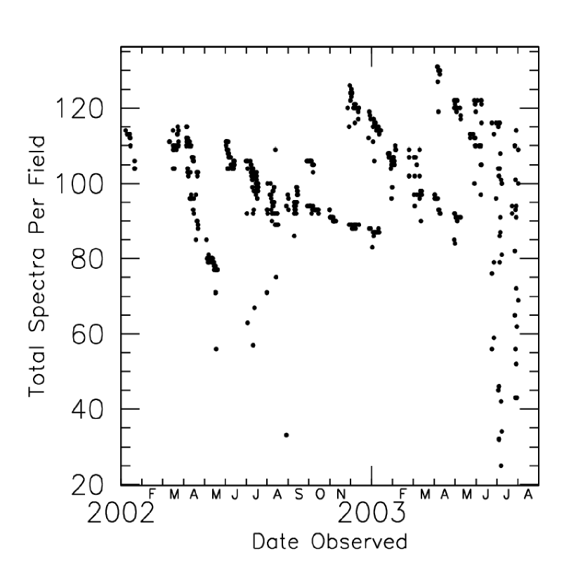
Figure 2: Total number of spectra obtained per field between January 2002 and June 2003. The upper envelope shows the maximum number of fibres available at any one time. It tracks the loss of fibres over time, and how Field plate #1 was taken out of service for January-February 2003 for a major fibre repair. The large scatter seen from the end of June 2003 is due to a change in observing strategy, from field choice maximising fibre allocation to one aimed at completing areas of sky.

Figure 3 shows the relationships between the full source list (top), those that remained unobserved at the time of the version D tiling allocation (middle), and the optimal tile placement to cover these (bottom).

Tests of the two-point correlation function were made on the sample selected through the final tiling allocation, to see what systematic effects might arise from its implementation. Mock catalogues were generated, with correlation function as observed by the 2dF Galaxy Redshift Survey (Hawkins et al. 2003), these were tiled as the real data and the resulting 2-point correlation function determined and compared with the original. This revealed an undersampling on scales up to $\sim 1$ $\,h\,{\rm Mpc}^{-1}$, clearly the result of the fibre button proximity limit. No bias was seen on larger scales.

Theoretical tiling completenesses of around 95% were achievable for all except the lowest priority samples, and variations in uniformity were confined to $<5$%. However, fibre breakages have meant that 6dFGS has consistently run with many fewer fibres than anticipated, impacting on the completeness of the lower priority samples in particular. With a fixed timeline for the survey (mid 2005) and a fixed number of fields to observe, there is little choice in the matter.

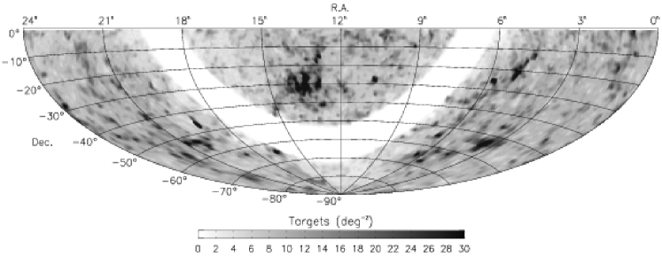
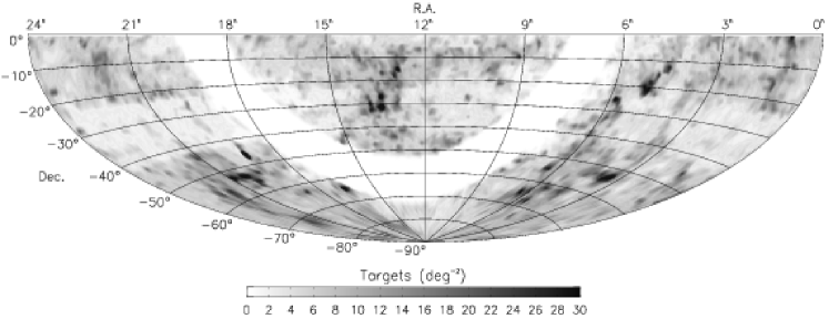
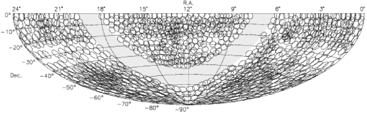
Figure 3: (top) Sky distribution of all targets in the source catalogues. (middle) Distribution of unobserved sources at the time of the version D tiling allocation in February 2003. Note how most of the fields observed between the versions A and D were confined to the central strip ($-23^{\circ}$ to $-42^{\circ}$ declination). (bottom) Optimal distribution of tiles based on the unobserved sources at the time of version D.

3.7 Fibre Assignment

Within each tile, targets are assigned to fibres by the same CONFIGURE software used by the 2dF Galaxy Redshift Survey. This iteratively tries to find the largest number of targets assigned to fibres, and the highest priority targets. Early configurations (until mid-2003) were usually tweaked by hand to improve target yield, after that date a revised version of CONFIGURE was installed with much improved yields and little or no further tweaking was in general made.

4 SURVEY IMPLEMENTATION

4.1 Observational Technique

Field acquisition with 6dF is carried out using conventional guide-fibre bundles. Four fibre buttons are fitted with coherent bundles of seven fibres rather than a single science fibre. Fibre diameter is 100$\mu$m (6.7″) and the guide fibres are in contact at the outer cladding to give a compact configuration $\sim$20 arcsec in diameter. These fibres are 5 m long and feed the intensified CCD acquisition camera of the telescope. The use of acquisition fibres of the same diameter as the science fibres is sub-optimal, but in practice the four guide-fibre bundles give good alignment, particularly as guide stars near the edge of the field are always chosen.

Guide stars are selected from the Tycho-2 catalogue (Hoeg et al. 2000), and have magnitudes typically in the range $8<V<11$. Field acquisition is straightforward in practice, and the distortion modelling of the telescope’s focal surface is sufficiently good that a field rotation adjustment is not usually required, other than a small standard offset.

Each field is observed with both V and R gratings, these are later spliced to reconstruct a single spectrum from these two observations. Integrations are a minimum of 1 hr for the V spectrum and 0.5 hr for the R spectrum, although these times are increased in poor observing conditions. This gives spectra with typical S/N around 10 pixel^-1, yielding $>$90% redshift completeness.

This observing strategy typically allows 3-5 survey fields to be observed on a clear night, depending on season. With 75% of the UKST time assigned to 6dFGS, and an average clear fraction of 60%, we typically observe about 400 fields per year. The observational strategy is to divide the sky into three declination strips. Initially, the survey has concentrated on the $\delta=-30^{\circ}$ declination strip (actually $-42^{\circ}<\delta<-23^{\circ}$); the equatorial strip ($-23^{\circ}<\delta<0^{\circ}$) will be done next, and then finally the polar cap ($\delta<-42^{\circ}$).

Observations started in June 2001, though final input catalogues and viable reduction tools were not available until 2002. Early data suffered from various problems, including poorer spectrograph focus due to misalignment within the camera; poorer quality control; and use of preliminary versions of the 2MASS data, leading to many observed sources being dropped from the final sample. The 2001 data are not included in this data release.

Initial observations were carried out at mid-latitudes for observational convenience, with the actual band corresponding to one of the Additional Target samples. Excursions from this band were made to target other Additional Target areas, where separate telescope time had been allotted to such a program, but the observations could be fruitfully folded in to 6dFGS.

The observing sequence conventionally begins with R data (to allow a start to be made in evening twilight). With the telescope at access park position, a full-aperture flat-field screen is illuminated with calibration lamps. First of these is a set of quartz lamps to give a continuum in each fibre. This serves two purposes; (a) the loci of the 150 spectra are defined on the CCD, and (b) the differences between the extracted spectra of the smooth blackbody lamp allow flatfielding of the signatures introduced into the object spectra by pixel-to-pixel variations and fibre-fibre chromatic throughput variations. Then the wavelength-calibration lamps are exposed, HgCd + Ne for the R data and HgCd + He for the V data. After the R calibration exposure, the field is acquired and the 3$\times$10-min red frames obtained. Once they are completed, the grating is changed remotely from the control room and the 3$\times$20-min V frames obtained. At the end of the sequence, the V wavelength calibration and flat-field exposures are made.

With the change of field comes a change of slit-unit (because of the two 6dF field plates), so all the calibrations must be repeated for the next field. Usually, the reverse waveband sequence is followed, i.e., beginning with V and ending with R. This process continues throughout the night, as conditions allow.

4.2 Reduction of Spectra

The reduction of the spectra uses a modified version of the 2DFDR package developed for the 2dF Galaxy Redshift Survey. Unlike 2dF data, tramline fitting is done completely automatically, using the known gaps in the fibres to uniquely identify the spectra with their fibre number. Because of computing limitations, TRAM rather than FIT extractions are performed. FIT extractions would reduce crosstalk between fibres, but this is already small for 6dF compared with 2dF. Scattered light subtraction is not in general performed, unless there is specific reason for concern, such as during periodic oil-contamination episodes within the dewar. Again, scattered light performance is better with 6dF in general than with 2dF.

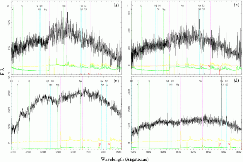
Figure 4: Examples of galaxy spectra from the 6dFGS exhibiting a range of types and redshift quality $Q$: ($a$) $Q=3$ ABS at $z=0.04601$. ($b$) $Q=3$ EMI at $z=0.03377$. ($c$) $Q=4$ ABS at $z=0.05645$. ($d$) $Q=4$ EMI at $z=0.05344$. Here, EMI refers to emission-line redshifts (and qualities), and ABS refers to absorption line determinations. Major absorption and emission-line features in the spectra have been labelled.

The extracted spectra for each field are combined, usually weighted by S/N to cope with variable conditions. The S/N is computed at this stage, and a S/N per pixel of 10 in each of V and R frames usually indicates a satisfactorily observed field. All data are then fluxed using 6dF observations of the standard stars Feige 110 and EG274. This fluxing is inevitably crude, in that the same fixed average spectral transfer function is assumed for each plate for all time. Differences in the transfer function between individual fibres are corrected for by the flat-fielding.

The resulting R and V spectra for each source are then spliced together, using the overlapping region to match their relative scaling. In order to avoid a dispersion discontinuity at the join in each spectrum, we also rescrunch the lower dispersion R data onto an exact continuation of the V wavelength dispersion.

4.3 Spectral Quality

Most spectra have no problems, in the sense that: (1) the S/N is reasonable given the magnitude of the source; (2) both V and R frames are available; and (3) there were no problems in the reduction. However, there are significant caveats of which all users should be aware.

• Many fields were observed in marginal conditions, and have reduced overall S/N as a result. Our philosophy has been to extract what good spectra we can from these fields, and recycle the rest for reobservation. A field was only reobserved in its entirety where the data was valueless.

• Many fields were observed with three or occasionally even two guide fibres, with consequent lower and more variable S/N.

• Some fibres have poor throughputs due to misalignment or poor glueing within the button, and variations of factors of two are normal.

• Many fibres, throughout the duration of the survey, have suffered various damage in use, short of breakage. Very often, this has resulted in strong fringing in the spectral response of the fibre, due to an internal fracture acting as a Fabry-Perot filter. This did not often flat-field out completely.

• The CCD is in any case a thinned blue-sensitive chip; as a result, red data suffers increasing levels of fringing towards longer wavelengths, and this does not always flat-field out.

• Fibre breakages during configuring, or between blue and red observations, or severe differences in acquisition, can lead to occasional missing or mis-spliced red or blue data.

• Some fields have missing red data.

• Though scattered light is not a major problem in general, data at the blue end of the spectra can be corrupted, because the actual counts are so low. In extreme cases, the spectra can become negative. The overall quality of the fluxing is untested, and should be treated with extreme caution.

• All VPH data suffer from a faint but variable, spurious, spectral feature at wavelengths around 4440 Å (10 pixel region) in the V grating, and 6430 and 6470 Å (10 pixel regions) in the R. The reason, after extensive investigation, was determined to be a ghost caused by dispersed light reflected back off the grating and recollimated by the camera, being undispersed in first order reflection mode by the VPH grating, and refocused onto the chip as a somewhat out-of-focus (10-20 pixel diameter), undispersed, image of the fibre, with an intensity 0.1-1% of the summed dispersed light. Circumventing this problem requires tilting the fringes within the grating (so they are no longer parallel with the normal to the grating) by a degree or two, to throw the ghost image just off the chip.

4.4 Redshift Measurement

Accurate redshift measurement is a fundamental componenent of both the $z$ and $v$-surveys. We started with the semi-automated redshifting RUNZ software used for the 2dF Galaxy Redshift Survey (Colless et al. 2001b), kindly provided by Will Sutherland. Extensive modifications were made in order to accept 6dF data. The version used for 2dF determined quasi-independent estimators of the redshift from emission and absorption features; this improved the reliability of the redshift estimates, while reducing their accuracy. Since the line identication of the higher S/N and higher dispersion 6dF spectra was usually not in doubt, we decided in general not to patch out emission features in determining cross-correlation redshifts; and in general the cross-correlation redshift was used in preference to the emission-line redshift.

Figure 5: Distribution of signal-to-noise for each class of redshift quality ($Q=1$ to 4) for the 6dFGS. The $Q=5$ sources are too few (24) to show.

Each automated redshift is checked visually to decide whether the software has made an accurate estimate or been misled by spurious spectral features. Such features are typically due to fibre interference patterns or poor sky subtraction and are difficult to identify through software, although easily recognisable to a human operator. The operator checks the automated redshift by comparing it to the original spectrum, the location of night-sky line features and the cross-correlation peak. In some cases, manual intervention in the form of re-fitting of spectral features or of the correlation peaks makes for a new redshift. In the majority of cases, however, the automated redshift value is accepted without change. The final redshift value is assigned a quality, $Q$, between 1 to 5 where $Q=3,4,5$ for redshifts included in the final catalogue. $Q=4$ represents a reliable redshift while $Q=3$ is assigned to probable redshifts; $Q=2$ is reserved for tentative redshift values and $Q=1$ for spectra of no value. $Q=5$ signifies a ‘textbook’ high signal-to-noise spectrum, although in practice is used rarely for the 6dFGS. Figure 4 shows a few examples of galaxy spectra across the range of redshift quality, for both emission and absorption-line spectra.

The same visual assessment technique was employed for the 2dF Galaxy Redshift Survey and greatly increased the reliability of the final sample: repeat measurements on a set of $\sim 15\,000$ 2dF spectra by two operators were discrepant in only 0.4% of cases (Colless et al. 2001b). Figure 5 shows the relationship between redshift quality $Q$ and mean signal-to-noise of the spectra that yielded them. The vast majority (76%) of the 6dFGS redshifts have $Q=4$ from spectra with a median signal-noise of 9.4  pixel^-1. The $Q=5$ sources are too few (24) to show. For $Q=3$ redshifts the median signal-to-noise ratio drops to 5.3  pixel^-1, indicating minimum of range of redshift-yielding spectra. In both cases, note the long tail to higher signal-to-noise values. The median signal-to-noise ratio for $Q=2$ redshifts (6.3  pixel^-1) is slightly higher than that for $Q=3$ (5.3  pixel^-1). This is due to the significant number of Galactic sources such as stars and planetary nebulae, which produce high signal-to-noise spectra, but are assigned $Q=2$ on account of their zero redshift.

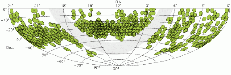
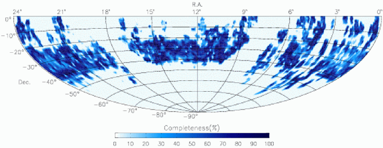
Figure 6: (top) Location of the observed fields contributing redshifts to the First Data Release. (bottom) Redshift completeness on the sky, combining the 6dF First Data Release redshifts with the literature sources.

5 FIRST DATA RELEASE

5.1 Statistics and Plots

Between January 2002 and July 2003 the 6dF Galaxy Survey Database compiled 52 048 spectra from which 46 474 unique redshifts were derived. The numbers of spectra with redshift quality $Q\geq 3$ were 43 945 for the full set and 39 649 for the unique redshifts. Of the 174 442 total galaxies in the target sample, 28 014 had existing literature redshifts: 19 570 from the ZCAT compilation (Huchra et al. 1999) and 8 444 from the 2dF Galaxy Survey (Colless et al. 2001b). Of the 113 988 $K_{s}$-selected sources, there are 32 156 6dF-measured redshifts of redshift quality $Q\geq 3$, plus a further 21 151 existing literature redshifts. Table 3 summarises these values for the individual sub-samples as they appear in the 6dFGS Database.

Table 3: Status of the 6dFGS target samples, as listed in the database.

id	survey	total	$cz\leq 600$	$cz>600$	6df $z$	lit $z$	6df$>600$	Q345	Q1	Q2	Q3	Q4	Q5	no $z$
1	2MASS $K_{s}<12.75$	113988	1750	53051	33650	21151	32983	32156	1312	1494	2708	29433	15	59187
3	2MASS $H<13.05$	3282	18	853	526	345	512	492	33	34	58	434	0	2411
4	2MASS $J<13.75$	2008	17	552	333	236	319	304	14	29	28	276	0	1439
5	DENIS $J<14.00$	1505	11	259	124	146	117	111	26	13	27	84	0	1235
6	DENIS $I<14.85$	2017	96	191	150	137	63	63	18	87	10	53	0	1730
7	SuperCOSMOS $r_{F}<15.6$	9199	137	3310	1539	1908	1439	1407	46	132	104	1302	1	5752
8	SuperCOSMOS $b_{J}<16.75$	9749	35	3718	1973	1780	1961	1900	76	73	173	1726	1	5996
78	Durham/UKST extension	466	2	73	10	65	8	8	1	2	6	2	0	391
90	Shapley supercluster	939	9	323	282	50	273	250	22	32	48	202	0	607
113	ROSAT All-Sky Survey	2913	99	535	395	239	300	223	231	172	53	170	0	2279
116	2MASS red AGN Survey	2132	9	252	129	132	121	81	106	48	45	36	0	1871
119	HIPASS ($>4\sigma$)	821	8	268	135	141	130	121	11	14	29	92	0	545
125	SUMSS/NVSS radio sources	6843	321	709	654	376	347	322	89	332	51	270	1	5813
126	IRAS FSC ($6\sigma$)	10707	258	2872	1360	1770	1218	1105	303	255	198	906	1	7577
129	Hamburg-ESO Survey QSOs	3539	73	197	220	50	150	56	204	164	19	37	0	3269
130	NRAO-VLA Sky Surv. QSOs	4334	342	146	483	5	142	62	303	421	42	20	0	3846
	Total	174442	3185	67309	41963	28531	40083	38661	2795	3302	3599	35043	19	103948

Column Headings:
$cz\leq 600$ — object has a redshift (either 6dF-measured with quality $>1$ or from the literature) less than or equal to 600 km s^-1.

$cz>600$ — object has a redshift (either 6dF-measured with quality $>1$ or from the literature) greater than 600 km s^-1.

6df $z$ — total number of 6dF-measured redshifts with quality $Q>1$.

lit $z$ — total number of literature redshifts.

6df$>600$ — number of 6dF-measured redshifts greater than 600 km s^-1with quality $Q>1$.

Q345 — total number of (6dF-measured) sources with redshift quality $Q=3,4$ or 5.

Q1, Q2, Q3, … — total number of sources with redshift quality $Q=1$, $Q=2$, $Q=3$, etc.

no $z$ — number of sources in the database with neither a 6dF (quality $Q>1$) nor literature redshift.

Data from 524 fields have contributed to the first data release. As shown in Fig. 6 (top), the majority of these occupy the central declination strip between $-42^{\circ}<\delta<23^{\circ}$. Overall there are 1564 on the sky: 547 in the equatorial strip, 595 in the central strip, and 422 in the polar region. Figure 6 (bottom) shows the corresponding distribution of redshift completeness on the sky for the $K$-band sample. The redshift completeness, $R$, is that fraction of galaxies in the parent catalogue of 174 442 with acceptable ($Q\geq 3$) redshifts in a given area of sky, from whatever source,

$$R = \frac{N_{z}(\mn@boldsymbol{\theta})}{N_{p}(\mn@boldsymbol{\theta})}$$ (2)

$$= \frac{N_{{\rm lit}}(\mn@boldsymbol{\theta})+N_{{\rm 6dF}}(\mn@boldsymbol{\theta})}{N_{{\rm lit}}(\mn@boldsymbol{\theta})+N_{{\rm 6dF}}(\mn@boldsymbol{\theta})+N_{\rm Gal}(\mn@boldsymbol{\theta})+N_{\rm f}(\mn@boldsymbol{\theta})+N_{\rm r}(\mn@boldsymbol{\theta})}$$

Here, $N_{p}(\mn@boldsymbol{\theta})$ is the number of galaxies from the parent catalogue (per unit sky area) at the location $\mn@boldsymbol{\theta}$, and $N_{z}(\mn@boldsymbol{\theta})$ is the number with redshifts, either from 6dF ($N_{{\rm 6dF}}(\mn@boldsymbol{\theta})$) or the literature ($N_{{\rm lit}}(\mn@boldsymbol{\theta})$). Sources in the parent catalogue that have been redshifted and excluded are either stars, planetary nebulae/ISM features (both assigned $Q=2$), or failed spectra ($Q=1$). In Eqn. 2 their numbers are denoted by $N_{\rm Gal}(\mn@boldsymbol{\theta})$ and $N_{\rm f}(\mn@boldsymbol{\theta})$. The remaining sources are those yet to be observed, $N_{\rm r}(\mn@boldsymbol{\theta})$. Of the first $\sim 41\,000$ sources observed with 6dF, around 3% were stars, 1% were other Galactic sources, and 11% failed to yield a redshift.

The field completeness is the ratio of acceptable redshifts in a given field to initial sources, and hence is only relevant to targets observed with 6dF. It also excludes Galactic features like stars and ISM. Figure 7 shows the distribution of field completeness from the first 524 fields and its cumulate. This demonstrates that the redshift success rate of 6dF is good, with both the median and mean completeness around 90%.

Figure 7: Galaxy redshift completeness by field, where completeness is the number of 6dF redshifts over the total 6dF redshifts and failures. The dashed line indicates the cumulative fraction according to the right-hand axis.

Observe the large difference between the high field completeness values of Fig. 7 and the lower redshift completeness in Fig. 6 (bottom). This is due to the high degree of overlap in the 6dFGS field allocation. The large variance in the density of targets has meant that most parts of the sky need to be tiled two or more times over. This is not at all obvious in Fig. 6 (top) which superimposes all fields, giving the impression of a single layer of tiles. While much of the central strip contains observed and redshifted fields, it also contains other fields in this same region, as yet unobserved.

The distribution of 6dFGS redshifts exhibits the classic shape for magnitude-limited surveys of this kind (Fig. 8). The median survey redshift, $\langle cz\rangle=16\,008$  km s^-1 ($\bar{z}=0.055$), is less than half that of the 2dFGRS or SDSS surveys.

Figure 8: Distribution of redshifts for the 6dF First Data Release galaxies with redshift quality $Q\geq 3$ and $cz>600$  km s^-1. The mean redshift for the survey ($\langle cz\rangle=16\,008$  km s^-1) is indicated with a vertical solid line.

Figure 9 shows the radial distribution of galaxies across the southern sky, projected across the full range of southerly declinations ($\delta=0$ to $-90^{\circ}$). Projecting in this way has the drawback of taking truly separate 3D space structures and blending them on the 2D page. Figure 10 shows the same data plotted $\Delta\delta=10^{\circ}$ declination slices and a magnified view of the lowest redshift galaxies within $-40^{\circ}<\delta<-30^{\circ}$.

Variations in galaxy density apparent in Figs. 9 and 10 are due the incomplete coverage of observed fields and the projection of the Galactic Plane. No 6dFGS galaxies lie within galactic latitude $|\,b\,|\leq 10^{\circ}$. The 6dFGS is also clumpier than optically-selected redshift surveys such as 2dFGRS and SDSS. This is because the near-infrared selection is biased towards early-type galaxies, which cluster more strongly than spirals.

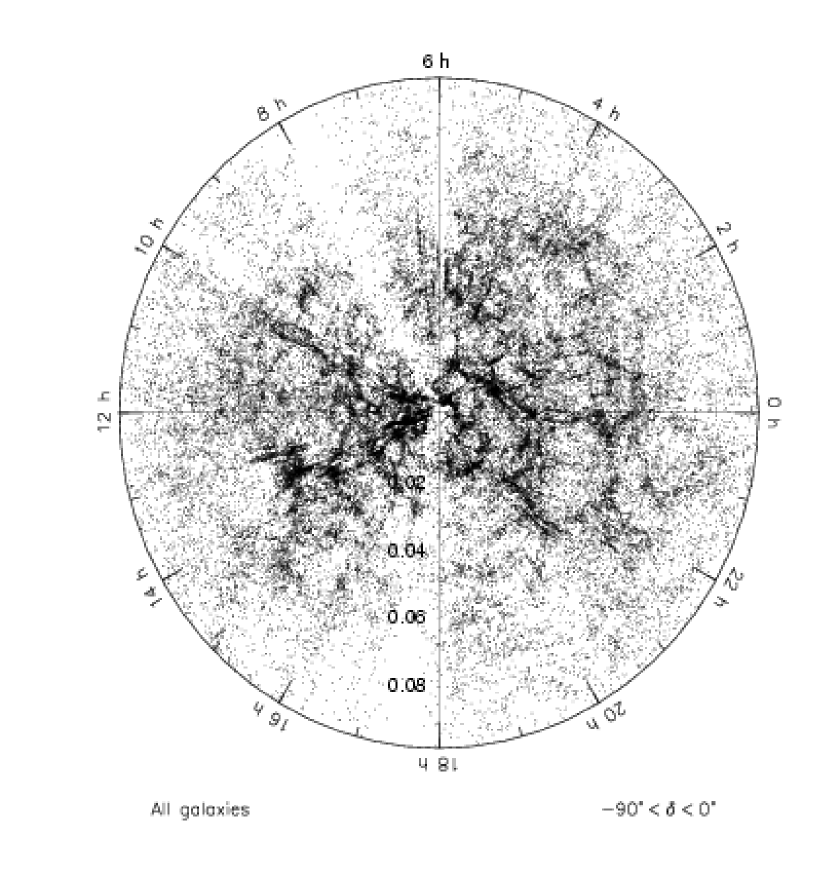
Figure 9: Spatial redshift distribution combining the 6dF and literature redshifts. The redshift slice projects through all southerly declinations, $\delta<0^{\circ}$. The sparse sampling around 8 and 17 hr is due to non-coverage in the Galactic Plane. Variations elsewhere in the sky are due to different sky regions having different observational completenesses at the time of this First Data Release.

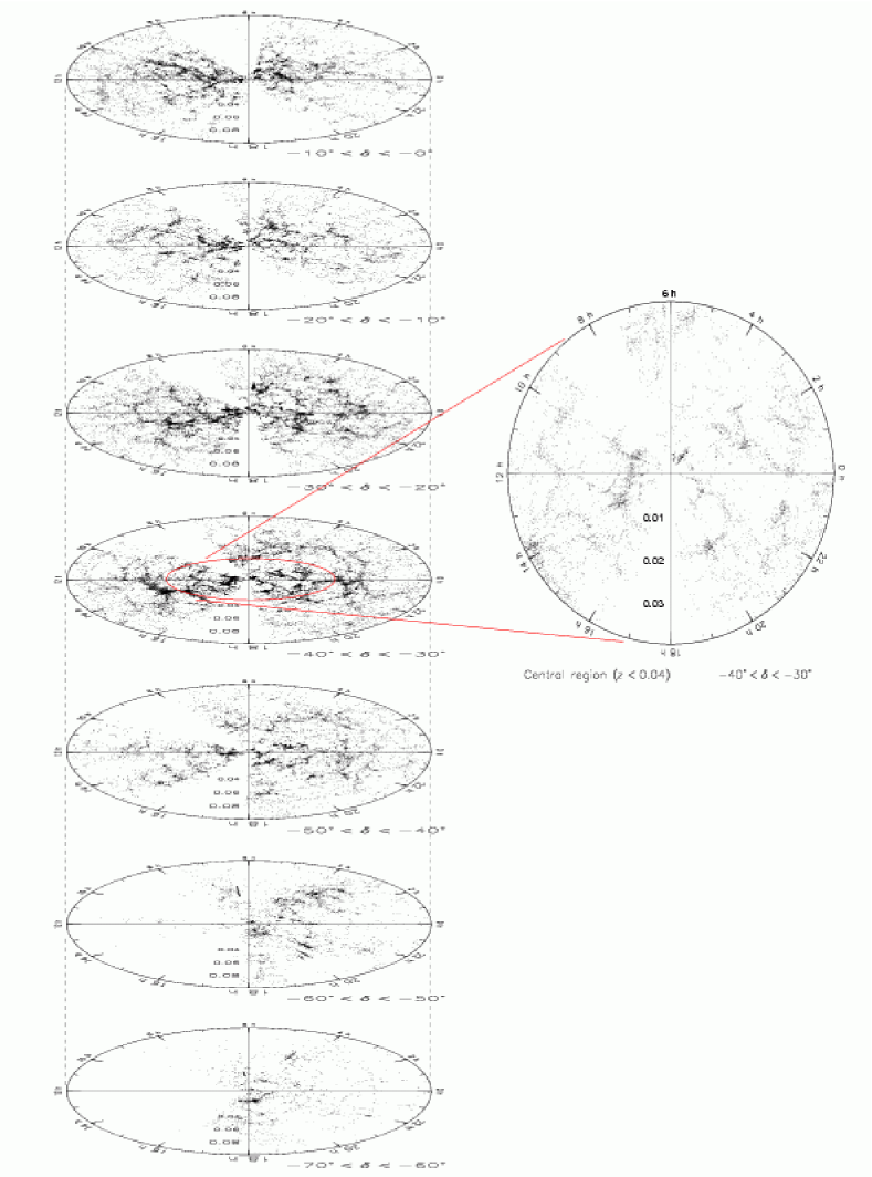
Figure 10: Spatial redshift distribution divided into discs, each spanning a $10^{\circ}$ range in declination. The inset shows an expanded view of the central region of the $-40^{\circ}<\delta<-30^{\circ}$ slice.

The 6dFGS provides the largest sample of near-infrared selected galaxies to determine the fraction of mass in the present-day universe existing in the form of stars. To this end, Jones et al. (2004) are deriving the $J$, $H$ and $K_{\rm s}$-band luminosity functions from the first 75 000 redshifts of the 6dF Galaxy Survey, combining data from both before and after the First Data Release. Using the near-infrared luminosity functions and stellar population synthesis models, the galaxy stellar-mass function for the local universe can be estimated. When this is integrated over the full range of galaxy masses, the total mass of the present-day universe in stars can be expressed in units of the critical density.

5.2 6dFGS Online Database

Data from the 6dF Galaxy Survey are publicly accessible through an online database at http://www-wfau.roe.ac.uk/6dFGS/, and maintained by the Wide Field Astronomy Unit of the Institute for Astronomy, University of Edinburgh. An early data release of around 17 000 redshifts was made in December 2002, along with the opening of the web site and tools for catalogue access. This paper marks the First Data Release of 52 048 total redshifts measured between January 2002 and July 2003. The design of the database is similar to that used for the 2dF Galaxy Redshift Survey in that parameterised data are stored in a relational database. Each TARGET object is also represented by a multi-extension FITS file which holds thumbnail images of the object and the spectra. The database is accessed/queried using Structured Query Language (SQL). A combined 6dF-literature redshift catalogue is provided in a separate single master catalogue.

The 6dFGS database is housed under Microsoft’s relational database software, SQL Server 2000. The data are organised in several tables (Table 4). The master target list used to configure 6dFGS observations is represented by the TARGET table. Spectral observations are stored in the SPECTRA table. The input catalogues that were merged to make up the master target list are also held in individual tables (TWOMASS, SUPERCOS etc.). The TARGET table forms the hub of the database. Every table is interlinked via the parameters targetid and targetname. These parameters are unique in the master TARGET table but are not necessarily unique in the other tables, (e.g. SPECTRA) as objects can and have been observed more than once. The SPECTRA table holds all the observational and redshift related data. Parameters are recorded for both the V and R frames (with a lot of the values being the same for both frames), and redshift information is derived from the combined VR frame. The TWOMASS table contains the $K$, $J$ and $H$-selected samples originating from the 2MASS extended source catalogue. The $K$-selected sample represents the primary 6dFGS input catalogue. Table 4 lists the programme details for the other contributing samples.

Initially every FITS file, representing each target (targetname.fits), holds thumbnail images of the target. As data are ingested into the database the reduced spectra are stored as additional FITS image extensions. Table 5 summarises the content within each FITS extension. The first 5 extensions contain the thumbnail images and each have a built-in World Coordinate System (WCS). The optical $B$ and $R$ images come from SuperCOSMOS scans of blue ($b_{\rm\scriptscriptstyle J}$) and red ($r_{\rm\scriptscriptstyle F}$) survey plates. The 2MASS $J$, $H$ and $K$ images were extracted from datacubes supplied by IPAC. Note that although some objects in TARGET do not have 2MASS images, the corresponding extensions still exist in the FITS file but contain small placeholder images. The remaining extensions contain the spectra. Each 6dFGS observation will usually result in a further 3 extensions, the V grating spectrum, the R spectrum and the combined/spliced VR spectrum.

Table 4: Tables of data in the 6dFGS Database

Table name	Description	Programme
		ID Numbers
TARGET	the master target list	progid
SPECTRA	redshifts and observational data	$-$
TWOMASS	2MASS input catalogue $K$, $H$, and $J$	1, 3, 4
SUPERCOS	SuperCOSMOS bright galaxies $b_{J}$ and $r_{F}$	7, 8
FSC	sources from the IRAS FAINT Source Catalogue	126
RASS	candidate AGN from the ROSAT All-Sky Survey	113
HIPASS	sources from the HIPASS HI survey	119
DURUKST	extension to Durham/UKST galaxy survey	78
SHAPLEY	galaxies from the Shapley supercluster	90
DENISI	galaxies from DENIS $I<14.85$	6
DENISJ	galaxies from DENIS $J<13.85$	5
AGN2MASS	candidate AGN from the 2MASS red AGN survey	116
HES	candidate QSOs from the Hamburg/ESO Survey	129
NVSS	candidate QSOs from NVSS	130
SUMSS	radio source IDs from SUMSS and NVSS	125

The V and R extensions are images with 3 rows. The 1st row is the observed reduced SPECTRUM, the 2nd row is the associated variance and the 3rd row stores the SKY spectrum as recorded for each data frame. Wavelength information is provided in the header keywords CRVAL1, CDELT1 and CRPIX1, such that

$${\rm wavelength\,(\AA)} = {\tt CRVAL1}-({\tt CRPIX1}-{\rm pixel\,number})$$ (3)

$$\times\,{\tt CDELT1}.$$

Additional WCS keywords are also included to ensure the wavelength information is displayed correctly when using image browsers such as Starlink’s GAIA or SAOimage DS9.

The VR extension also has an additional 4th row that represents the WAVELENGTH axis, which has a continuous dispersion, achieved through the continuation of the V dispersion into the R half from rescrunching.

Table 5: Contents of each extension in the database FITS files

FITS	Contents
Extension
1st	SuperCOSMOS $b_{\rm\scriptscriptstyle J}$ image ($1\times 1$ arcmin)
2nd	SuperCOSMOS $r_{\rm\scriptscriptstyle F}$ image ($1\times 1$ arcmin)
3rd	2MASS $J$ image (variable size)
4th	2MASS $H$ image (variable size)
5th	2MASS $K$ image (variable size)
6th	V-spectrum extension
7th	R-spectrum extension
8th	combined VR-spectrum extension
$n$th	additional V, R, and VR data

Access to the database is through two different Hypertext Mark-up Language (HTML) entry forms. Both parse the user input and submit an SQL request to the database. For users unfamiliar with SQL, the menu driven form provides guidance in constructing a query. The SQL query box form allows users more comfortable with SQL access to the full range of SQL commands and syntax. Both forms allow the user to select different types of output (HTML, comma separated value (CSV) or a TAR save-set of FITS files).

There are online examples of different queries using either the menu or SQL form at http://www-wfau.roe.ac.uk/6dFGS/examples.html. More information about the database is available directly from the 6dFGS database website.

6 CONCLUSIONS

The 6dF Galaxy Redshift Survey (6dFGS) is designed to measure redshifts for approximately 150 000 galaxies and the peculiar velocities of 15 000. The survey uses the 6dF multi-fibre spectrograph on the United Kingdom Schmidt Telescope, which is capable of observing up to 150 objects simultaneously over a $5.7^{\circ}$-diameter field of view. The 2MASS Extended Source Catalog (Jarrett et al. 2000) is the primary source from which targets have been selected. The primary sample has been selected with $K_{\rm tot}\leq 12.75$, where $K_{\rm tot}$ denotes the total $K$-band magnitude as derived from the isophotal 2MASS $K$ photometry. Additional galaxies have been selected to complete the target list down to $(H,J,r_{F},b_{J})=(13.05,13.75,15.6,16.75)$. Thirteen miscellaneous surveys complete the total target list.

The survey covers the entire southern sky (declination $\delta<0^{\circ}$), save for the regions within $|\,b\,|\leq 10^{\circ}$ of the Galactic Plane. This area is has been tiled with around 1500 fields that effectively cover the southern sky twice over. An adaptive tiling algorithm has been used to provide a uniform sampling rate of 94%. In total the survey covers some 17 046 deg² and has a median depth of $\bar{z}$=0.05. There are three stages to the observations, which initially target the declination strip $-42^{\circ}<\delta<-23^{\circ}$, followed by the equatorial region $-23^{\circ}<\delta<0^{\circ}$, and conclude around the pole, ($\delta<-42^{\circ}$).

Spectra are obtained through separate V and R gratings and later spliced to produce combined spectra spanning 4000 – 8400 Å. The spectra have 5 – 6 Å FWHM resolution in V and 9 – 12 Å resolution in R. Software is used to estimate redshifts from both cross-correlation with template absorption-line spectra, and linear fits to the positions of strong emission lines. Each of these automatic redshift estimates is checked visually and assigned a quality $Q$ on a scale of 1 to 5, where $Q\geq 3$ covers the range of reliable redshift measurements. The median signal-to-noise ratio is 9.4  pixel^-1 for redshifts with quality $Q=4$, and 5.3  pixel^-1 for $Q=3$ redshifts.

The data in this paper constitute the First Data Release of 52 048 observed spectra and the 46 474 unique extragalactic redshifts from this set. The rates of contamination by Galactic and failed spectra are 4% and 11% respectively. Data from the 6dF Galaxy Survey are publicly available through an online database at http://www-wfau.roe.ac.uk/6dFGS/, searchable through either SQL query commands or a online WWW form. The main survey web site can be found at http://www.mso.anu.edu.au/6dFGS.

References

- (1) Blanton, M.R. et al., 2001, AJ, 121, 235
- (2) lanton, M.R. et al., 2003, AJ, 125, 2276
- (3) Branchini, E. et al., 1999, MNRAS, 308, 18
- (4) Burkey, D., 2004, PhD dissertation, in prep.
- (5) Burkey, D. & Taylor, A., 2004, MNRAS, submitted
- (6) Campbell, L.A. et al., 2004, MNRAS, in press
- (7) Cole S. et al., (2dFGRS team), 2001, MNRAS, 326, 255
- (8) Colless, M.M. et al., 2001a, MNRAS, 321, 277
- (9) Colless, M.M. et al., (2dFGRS team), 2001b, MNRAS, 328, 1039
- (10) Cross, N. et al., (2dFGRS team), 2001, MNRAS, 324, 825
- (11) da Costa, L.N. et al., 2000, ApJ, 537, L81
- (12) De Propris, R. et al., (2dFGRS team), 2002, MNRAS, 329, 87
- (13) Djorgovski, S. & Davis, M., 1987, ApJ, 313, 59
- (14) Dressler, A. et al., 1987, ApJ, 313, 42
- (15) Efstathiou, G. et al., (2dFGRS team), 2002, MNRAS, 330, 29
- (16) Folkes, S. et al., (2dFGRS team), 1999, MNRAS, 308, 459
- (17) Giovanelli, R. et al., 1998, AJ, 116, 2632
- (18) Goto T. et al., 2003, PASJ, 55, 739
- (19) Hambly, N.C. et al., 2001, MNRAS, 326, 1279
- (20) Hawkins, E. et al., (2dFGRS team), 2003, MNRAS, 346, 78
- (21) Hoeg, E. et al., 2000, A&A, 355, L27
- (22) Huchra, J. et al., ApJS, 121, 287
- (23) Hudson, M.J. et al., 1999, ApJ, 512, L79
- (24) Jarrett, T.-H. et al., 2000, AJ 120, 298
- (25) Jones, D.H. et al., 2004, in prep.
- (26) Lahav, O. et al., (2dFGRS team), 2002, MNRAS, 333, 961
- (27) Lauer, T.R. & Postman, M., 1994, ApJ, 425, 418
- (28) Lewis, I.J. et al., 2002, MNRAS, 333, 279
- (29) Lynden-Bell, D. et al., 1988, ApJ, 326, 19
- (30) Madgwick, D.S. et al., (2dFGRS team), 2002, MNRAS, 333, 133
- (31) Metropolis, N. et al., 1953, J. Chem. Phys., 21
- (32) Norberg, P. et al., 2002, MNRAS, 336, 907
- (33) Parker, Q.A. et al., 1998, in Fiber Optics in Astronomy III, ASP Conf Series 152, p80
- (34) Parker, Q.A & Watson, F.G., 1995, in Fiber Optics in Astronomical Applications, Proc SPIE v2476, ed. S. Barden, p34
- (35) Peacock, J.A. et al., (2dFGRS team), 2001, Nature, 410, 169
- (36) Percival W.J. et al., (2dFGRS team), 2001, MNRAS, 327, 1297
- (37) Saunders, W. et al., 2000, MNRAS, 317, 55
- (38) Saunders W. et al., 2001, AAO Newsletter, 97, 14
- (39) Scaramella, R. et al., Nature, 338, 562
- (40) Szalay, A. et al., 2003, ApJ, 591, 1
- (41) Verde, L. et al., (2dFGRS team), 2002, MNRAS, 335, 432
- (42) Watson, F.G et al., 2000, in Optical and IR Telescope Instrumentation and Detectors, Proc SPIE vol 4008, eds. M. Iye, A.F. Moorwood, p123
- (43) Wegner, G.A. et al., 1999, MNRAS, 305, 259
- (44) York, D.G. et al., 2001, AJ 120, 1579
- (45) Zehavi, I. et al., (SDSS team), 2002, ApJ, 571, 172