Dissipation of Magnetic Flux in Primordial Gas Clouds

Abstract

We report the strength of seed magnetic flux of accretion disk surrounding the PopIII stars. The magnetic field in accretion disk might play an important role in the transport of angular momentum because of the turbulence induced by Magneto-Rotational Instability (MRI). On the other hand, since the primordial star-forming clouds contain no heavy elements and grains, they experience much different thermal history and different dissipation history of the magnetic field in the course of their gravitational contraction, from those in the present-day star-forming molecular clouds. In order to assess the magnetic field strength in the accretion disk of PopIII stars, we calculate the thermal history of the primordial collapsing clouds, and investigate the coupling of magnetic field with primordial gas. As a result, we find that the magnetic field strongly couple with primordial gas cloud throughout the collapse, i.e. the magnetic field are frozen to the gas as far as initial field strength satisfies $B\lesssim 10^{-5}(n_{\rm H}/10^{3}~{}{\rm cm^{-3}})^{0.55}~{}{\rm G}$.

1 INTRODUCTION

PopIII stars are considered to have very important impacts on the thermal history and the chemical evolution of the universe. Recent observations of the polarization of Cosmic Microwave Background (CMB) photons by WMAP(Wilkinson Microwave Anisotropy Probe) (Kogut et al. 2003) revealed that the optical depth of the universe by Thomson scattering is fairly large ($\tau=0.17\pm 0.04$). This result tells that reionization epoch is earlier ($z=17\pm 5$) than expected from the observations on Gunn-Peterson trough (Becker et al. 2001; Fan et al. 2002; White et al. 2003). On the other hand, the results of theoretical calculations of structure formation (Sokasian et al. 2003) indicate that such early reionization seems to be difficult solely by the Pop II stars, but it might be possible if the ionizing photons from PopIII stars with top heavy initial mass function (IMF) is taken into account. Thus, the mass (or IMF) of PopIII star have great significance on the reionization epoch of the universe. In addition, some amount of metals are found at high redshift intergalactic matter by the observation of high redshift QSO absorption line systems(Songaila 2001; Ma 2002; Vladilo 2002). This means significant fraction of baryons are already processed in the stars by $z=5$ (Songaila 2001). PopIII stars also should be responsible for such metal pollution of the early universe, and the abundance pattern of heavy elements depends on the mass of PopIII stars. Thus, typical mass (or IMF) of the PopIII stars is a key quantity also for the chemical evolution of the universe.

In order to assess the typical mass of PopIII stars, typical scale of the prestellar core (or fragments of primordial gas) should be evaluated as a first step. Several authors have studied on this issue by simple one-zone approach before middle of ’90s (Matsuda, Sato & Takeda 1969; Hutchins 1976; Carlberg 1981; Palla, Salpeter & Stahler 1983; Susa, Uehara & Nishi 1996; Uehara et al. 1996; Puy & Signore 1996). Recently, multi-dimensional numerical simulations of fragmentation of primordial gas have been performed intensively by several authors(Nakamura & Umemura 1999; Bromm, Coppi & Larson 1999; Abel, Bryan & Norman 2000; Nakamura & Umemura 2001; Bromm, Coppi & Larson 2002), and they find that the mass of PopIII prestellar core is quite massive ($\sim 10^{3-4}M_{\odot}$).

Further evolution of prestellar core was investigated by Omukai & Nishi (1998), and it is found that the collapse proceeds in a run-away fashion and converges to Larson-Penston similarity solution (Larson 1969; Penston 1969) with $\gamma\simeq 1.1$. They also find the mass accretion rate is also very large compared to the present-day forming stars, although spherical symmetry is assumed in their numerical calculation. In reality, however, prestellar cores have some amount of angular momentum, which prevent the mass from accreting onto the protostars. Consequently, accretion disks surrounding the protostars are expected, and some mechanisms that transport their angular momentum are required in order to enable the mass accretion onto protostars.

There are a few possibilities of the angular momentum transport such as gravitational torque by the nonaxisymmetric structures in the accretion disk, the interaction among the fragments of the disk (Stone et al. 2000; Bodenheimer et al. 2000), and the turbulent viscosity triggered by Magneto-Rotational Instability (MRI) (Hawley & Balbus 1992; Sano, Inutsuka & Miyama 1998; Sano & Inutsuka 2001). All of these mechanisms are regarded to be important for present-day star formation. Thus, it is worth to investigate these processes for primordial case. Among these possibilities, we concentrate on the last one, the MRI induced turbulence.

In order to activate MRI, the initial magnetic field strength in the accretion disk should be larger than a critical value. Otherwise the magnetic field is dissipated before the field is amplified by MRI (Tan & McKee 2004; Tan & Blackman 2004). Thus, it is important to assess the “initial” magnetic field strength in the accretion disk. As was discussed by Nakano & Umebayashi (1986) for preset-day case, magnetic field could be dissipated while prestellar core collapses. However, the dissipation processes strongly depend on the components of the gas as well as the the temperature evolution in the course of the collapse. On the other hand, the temperature of the collapsing primordial gas is much higher than that of the present-day case (Omukai 2000), which might bring about different dissipation history of the magnetic field.

In this paper, we investigate the dissipation of magnetic field in collapsing primordial gas cloud. Consequently, we obtain the initial magnetic field strength in the accretion disk of PopIII stars. In the next section, formulations are described. In §3, results of our calculations are shown, and the importance of MRI in PopIII star formation is discussed in §4. Final section is devoted to summary.

2 CALCULATIONS

We consider the collapse of spherical clouds without metals and dusts, but with slight magnetic fields. Then, we calculate the time evolution of the central density, chemical composition and dissipation of magnetic flux from the gravitationally collapsing core. The initial strength of magnetic fields when primordial clouds begin to contract is given as unknown parameter.

2.1 Dynamics

We assume that the dynamics is described by the free-fall relation,

$$\frac{d\rho}{dt}=\frac{\rho}{\tau_{\rm ff}},$$ (1)

where $\rho$ is the density of the collapsing core and $\tau_{\rm ff}=(3\pi/32G\rho)^{1/2}$ is the free-fall time. In fact, as described in Omukai (2000), thermal evolution of the core in 1D hydrodynamic simulation is well described by such one zone model. On the other hand, we also have to evaluate the dissipation of magnetic field in the accretion phase, and it is not the same as the case of collapsing core. In this case, the temperature of the accretion flow would rise faster than those in the core, because of shock heating. Thus, the magnetic field is expected to be frozen to the gas also in the accretion flow, if the frozen condition is satisfied in the collapsing core.

It is also worth noting that this free-fall approximation is also marginally valid for the case of quasi-hydrostatic core found in the simulation by Abel, Bryan & Norman (2000, 2002). In fact, panel C of Fig.3 in Abel, Bryan & Norman (2000) tells that the cooling time is as short as the free-fall time. Thus, the system evolves with time scale $\tau_{\rm ff}\simeq\tau_{\rm cool}$.

In order to describe thermal processes, we approximate the equation of state to be polytrope with index $\gamma=1.1$,

$$p=K\rho^{\gamma},$$ (2)

where $K$ is the constant coefficient. The reason to adopt the polytrope of $\gamma=1.1$ is that in past work the thermal evolution of primordial collapsing core is investigated in detail by Omukai (2000), where the temperature grows with $\gamma\sim 1.1$ in considering heating/cooling processes.

Since we are interested in the collapsing gas cloud, the magnetic energy density needs to be less than the gravitational energy density of the cloud core. The critical field strength $B_{\rm cr}$ is defined by the equation $B_{\rm cr}^{2}/4\pi R\simeq\rho GM/R^{2}$. Since the radius of the core should be on the order of Jean’s length, $B_{\rm cr}$ is given by the following equation,

$$B_{\rm cr} \simeq (3G)^{1/2}M_{\rm J}/R_{\rm J}^{2}$$ (3)

$$= (4/3)^{1/2}\pi^{3/2}c_{\rm s}\rho^{1/2}\propto\rho^{0.55},$$

where $R_{\rm J}$, $M_{\rm J}$, and $c_{\rm s}$ are the Jean’s length, the Jean’s mass, and the sound velocity, respectively.

2.2 Dissipation of Magnetic Fields

There are two processes for the dissipation of magnetic fields. The first one is Ohmic loss, and the other is ambipolar diffusion. We assess the degree of dissipation defined by the ratio of the drift velocity $v_{{\rm B}x}$ of the field lines from the gas to the free-fall velocity, as was introduced in Nakano & Umebayashi (1986). In Nakano & Umebayashi (1986), the drift velocity involves both the Ohmic dissipation and the ambipolar diffusion processes. There are two important quantities which characterize these diffusion processes. They are $\tau_{\nu}$ and $\omega_{\nu}$ which denote the viscous damping time of the relative velocity of charged particle $\nu$ to the neutral particles, and the cyclotron frequency of the charged particle $\nu$, respectively. Then, $\tau_{\nu}$ is expressed as

$$\tau_{\nu}=\frac{\rho_{\nu}}{\mu_{\rm\nu n}n_{\nu}n_{\rm n}\langle\sigma v\rangle_{\rm\nu n}},$$ (4)

where $\mu_{\rm\nu n}$ is the reduced mass, $n_{\nu}$, $n_{\rm n}$, and $\rho_{\nu}$ are, the mean number density for the charged particle $\nu$, the neutral particle ${\rm n}$, and the mass density of charged particle $\nu$, respectively. The averaged momentum-transfer rate coefficient for a particle $\nu$ colliding with a neutral particle is expressed by $\langle\sigma v\rangle_{\rm\nu n}$ .

The momentum-transfer cross section of an ion with a neutral particle is given by the Langevin rate coefficient (Osterbrock 1961). For an electron, it is found experimentally by Hayashi (1981) that the cross sections at low energies are much smaller than the Langevin rate coefficient and are nearly equal to a geometrical cross section. We use the empirical formulae for the momentum-transfer rate coefficients (Kamaya & Nishi 2000; Sano, Miyama, Umebayashi, & Nakano 2000).

According to Nakano & Umebayashi (1986), the drift velocity can be given by

$$v_{{\rm B}x}=\frac{A_{1}}{A}\frac{1}{c}(\mbox{\boldmath$j$}\times\mbox{\boldmath$B$})_{x},$$ (5)

where

$$A=A_{1}^{2}+A_{2}^{2},$$ (6)

$$A_{1}=\sum_{\nu}\frac{\rho_{\nu}\tau_{\nu}\omega_{\nu}^{2}}{1+\tau_{\nu}^{2}\omega_{\nu}^{2}},$$ (7)

$$A_{2}=\sum_{\nu}\frac{\rho_{\nu}\omega_{\nu}}{1+\tau_{\nu}^{2}\omega_{\nu}^{2}},$$ (8)

$B$ is the mean magnetic field in the primordial cloud, the suffix $x$ means $x$ direction component in local Cartesian coordinates where the $z$ direction is taken as the direction of $B$. In calculating the drift velocity $v_{{\rm B}x}$ according to equation (5) we replace $(1/c)(\mbox{\boldmath$j$}\times\mbox{\boldmath$B$})_{x}$ with the mean magnetic force $B^{2}/4\pi R$, where $B$ is the mean field strength in the cloud, $R$ is the radius of the cloud.

The magnetic field is mainly dissipated by the Ohmic loss when $|\tau_{\nu}\omega_{\nu}|<1$ for main charged particles. In such a situation we have the approximate expression from equations (5), (6), (7) and (8) that

$$v_{{\rm B}x}\sim\frac{c^{2}}{4\pi\sigma_{\rm c}R},$$ (9)

where $\sigma_{\rm c}$ the electrical conductivity,

$$\sigma_{\rm c}=\sum_{\nu}\frac{q_{\nu}^{2}\tau_{\nu}n_{\nu}}{m_{\nu}},$$ (10)

$q_{\nu}$ and $m_{\nu}$ are the electrical charge and the mass for a charged particle $\nu$, respectively. Thus the drift velocity is independent of $B$. On the other hand, when $|\tau_{\nu}\omega_{\nu}|>1$, the ambipolar diffusion is a main process of dissipation. In such a case we obtain

$$v_{{\rm B}x}\sim\frac{\tau_{\rm i}}{\rho_{\rm i}}\frac{B^{2}}{4\pi R},$$ (11)

where the suffix i expresses the ion particles. Note that the drift velocity is proportional to $B^{2}$ in this case.

Tan & Blackman (2004) have evaluated the drift velocity of magnetic field in the quasi-hydrostatic core found in Abel, Bryan & Norman (2000, 2002), when its density is a certain value. However, this system is highly non-equilibrium, and the ionization degree gets smaller and smaller as the collapse proceeds. Thus, its is not trivial at all whether the frozen condition is satisfied or not at much higher density. Therefore, we have to perform detailed non-equilibrium calculations of chemical reaction network, in order to obtain the correct ionization degree in the collapsing gas.

2.3 Chemistry

In order to investigate the evolution of ionized fraction during the collapse in detail, we solve non-equilibrium chemical reaction network of primordial gas that involves not only H element, but also D, He, and Li. Furthermore, we introduce following 24 species: ${\rm e^{-}}$, ${\rm H^{+}}$, H, ${\rm H^{-}}$, ${\rm H_{2}}$, ${\rm H_{2}^{+}}$, ${\rm H_{3}^{+}}$, D, ${\rm D^{+}}$, $\rm D^{-}$, HD, ${\rm HD^{+}}$, ${\rm H_{2}D^{+}}$, He, ${\rm He^{+}}$, ${\rm He^{++}}$, ${\rm HeH^{+}}$, Li, ${\rm Li^{+}}$, ${\rm Li^{++}}$, ${\rm Li^{3+}}$, ${\rm Li^{-}}$, LiH, and ${\rm LiH^{+}}$. We employ the latest reaction rate coefficients appearing in the following papers, Galli & Palla (1998), Omukai (2000), Stancil, Lepp & Dalgarno (1998), Flower (2002) and Lepp, Stancil & Dalgarno (2002). As for the radiative recombination, we use the rate coefficients based on Spitzer (1978).

2.4 Initial Conditions

We employ two different initial conditions A and B. For model A, we set $n_{\rm H,ini}=10^{3}\ {\rm cm^{-3}}$ and $T_{\rm ini}=250\ {\rm K}$ for initial conditions of prestellar core. We use the fraction of the chemical composition in the early universe given by Galli & Palla (1998) as the initial condition for the cloud. This model is on the evolutionary track ($Z=0$, fiducial model) in Omukai (2000). On the other hand, as was shown by Palla, Salpeter & Stahler (1983) and Omukai (2000), the paths in $n_{\rm H}-T$ plane rapidly converge to an identical trajectory from various initial conditions. Remark the almost hydrostatic prestellar core found in the numerical simulations in Abel, Bryan & Norman (2000) is also very close to the above trajectory. Thus, this choice of initial condition is quite natural for the formation of PopIII stars.

On the other hand, there is a case which do not converges rapidly to the trajectory, which was pointed out by Uehara & Inutsuka (2000) and Nakamura & Umemura (2002). In this case, the gas is initially heated up to 10⁴ K during the collapse of rather massive host galaxy, and H₂ is formed efficiently utilizing the residual electrons as catalysts (e.g. Susa et al. 1998). Afterwards, HD is formed from H₂, and the gas is cooled down to $\sim$100 K. Furthermore, the gas temperature is kept at relatively low level ($\sim 100$ K) in the course of the collapse. We employ this case as model B, in which we set the initial condition ($n_{\rm H,ini}=10^{3}\ {\rm cm^{-3}},T_{\rm ini}=100\ {\rm K}$), and the initial fractional abundances are taken from the results of Nakamura & Umemura (2002).

The initial magnetic field strength for the primordial star-forming environment has been investigated by many authors (e.g. Pudritz & Silk 1989; Kulsrud et al. 1997; Widrow 2002; Langer, Puget & Aghanim 2003). However, the initial field generation is still a controversial question. Thus, the initial magnetic field strength is given as the model parameter in our calculations.

3 RESULTS

3.1 Ionization degree

Figure 1 shows the fractional abundance of various species, e, ${\rm H}^{+}$, H, ${\rm H}_{2}$, ${\rm H_{3}^{+}}$, Li, and ${\rm Li}^{+}$ for model A. At low density, $n_{\rm H}\lesssim 10^{11}\ {\rm cm}^{-3}$, the ionization degree decreases as density increases because of the recombination of the electrons with the protons. However, since the ${\rm Li}^{+}$ recombination rate is smaller than that of ${\rm H}^{+}$, the reduction of the ionization degree is almost quenched at $n_{\rm H}\sim 10^{12}\ {\rm cm^{-3}}$. Moreover, the ionization degree increases at the higher density because the collisional ionization is activated by high temperature. Note that the ionization degree is very small, but there is a minimal value $\sim 10^{-12}$. Figure 2 shows the results for model B. In this case, the fraction of electrons evolve in a similar way. There is a minimal value $\sim 10^{-12}$, at which the electrons are provided by Li.

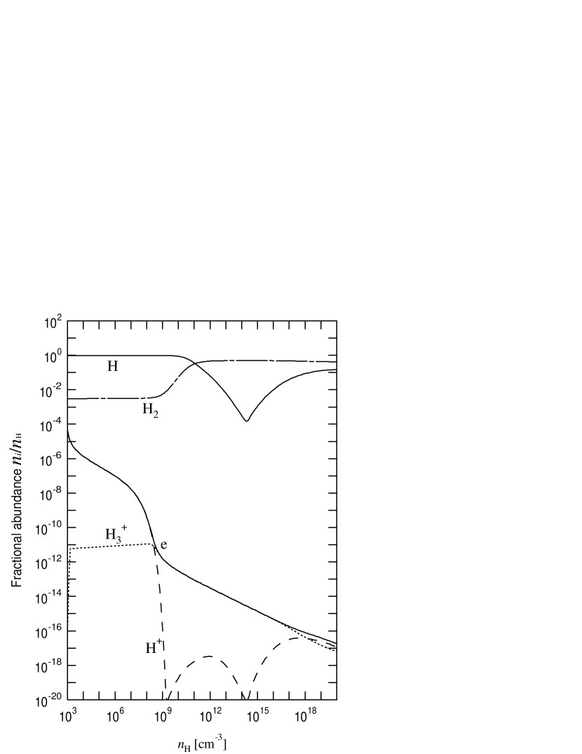
Figure 4: Same as Figure 2 except that this model is calculated without Li.

In order to clarify the importance of Li, we perform control runs without Li, ${\rm Li^{+}}$, ${\rm Li^{++}}$, ${\rm Li^{3+}}$, ${\rm Li^{-}}$, LiH, and ${\rm LiH^{+}}$, for both initial conditions A and B. The results of these runs are shown in Figures 3 and 4. In the case of model A, even without Li, ionized fraction do not gets smaller than $\sim 10^{-12}$(Figure 3). Therefore, presence of Li is not so important in this case. However, for the model B, the result is much different from the other case. In the presence of Li, electron fraction is kept around $10^{-12}$ even at $n_{\rm H}>10^{11}\ {\rm cm^{-3}}$. But in the absence of Li, electron fraction gets much smaller than $10^{-12}$ (Figure 4). Thus, Li is quite important in the low temperature model. We will come back to this point in the next subsection.

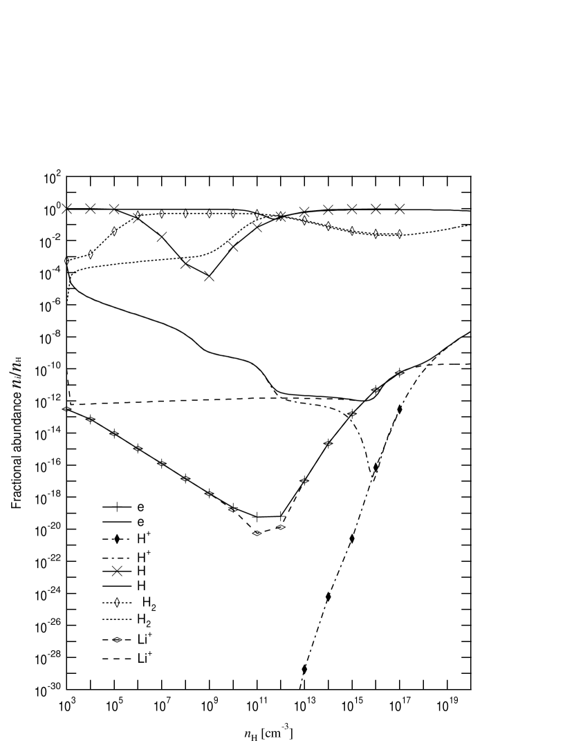
Figure 5: The fractions of various chemical species after the time integration assuming fixed density and temperature over $10^{3}\ {\rm Gyrs}$ are superimposed on Figure 1. Curves with markers represent the fractions after long time integration, and the unmarked curves represent the non-equilibrium fractions.

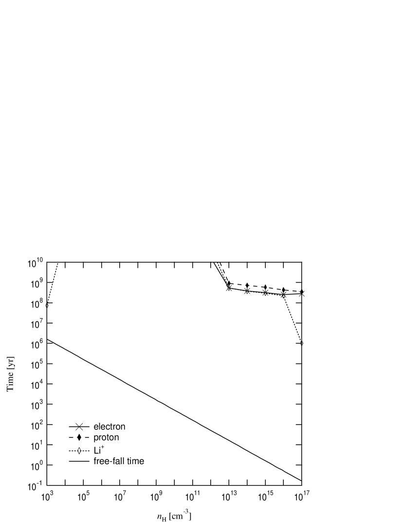
Figure 6: Time scale of equilibration is shown for several species.

We also emphasize the significance of non-equilibrium treatment of chemical reactions. Figure 5 shows the fractions of various chemical species after the time integration assuming fixed density and temperature over $10^{3}\ {\rm Gyrs}$ (a hundred times larger than the age of the universe). As a result, for $n_{\rm H}\gtrsim 10^{13}\ {\rm cm^{-3}}$, the fractions of chemical species converge to equilibrium values, although they are still not in equilibrium for lower densities. It is clear that results from non-equilibrium calculation is very different from those in chemical equilibrium. Especially, the non-equilibrium fraction of electron is much larger than the equilibrium value. The time scales of equilibration are also shown in figure 6, and they are always much longer than the local free-fall time. Thus, non-equilibrium calculations are indispensable to evaluate the ionization degree of collapsing primordial gas.

3.2 Drift velocity of magnetic field

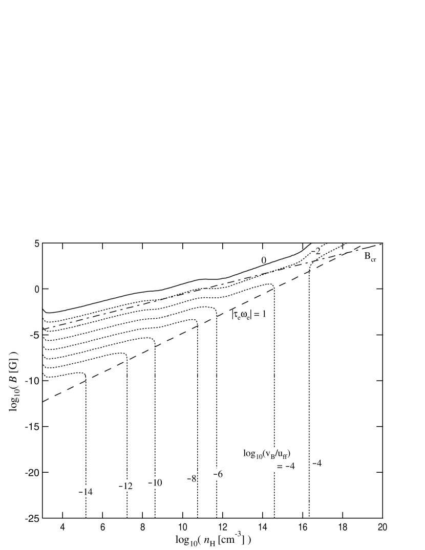
Figure 7: The drift velocity $v_{{\rm B}x}$ of the magnetic field as a function of the density $n_{\rm H}$ and the field strength $B$ for a collapsing cloud for model A. The dotted curves represent the contours of constant $v_{{\rm B}x}$ normalized by the free-fall velocity $u_{\rm ff}$ and its logarithmic values are labelled on those curves. The solid curve shows the locus along which $v_{{\rm B}x}=u_{\rm ff}$ is satisfied. The dashed line represents the locus $|\tau_{\nu}\omega_{\nu}|=1$ for electrons. The dot-dashed line represents the critical field $B_{\rm cr}$ given by equation (3).

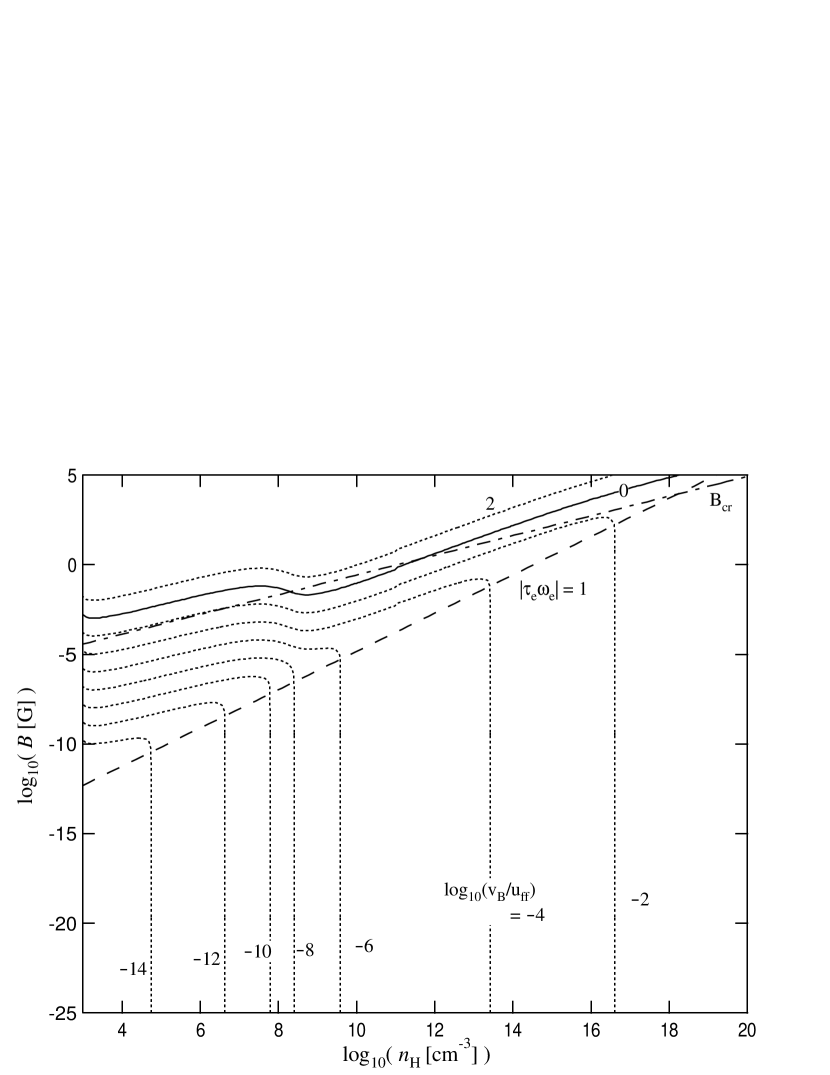
Figure 8: Same as Figure 7 except that the initial temperature is 100K (model B).

We calculate the drift velocity of magnetic field using the results of the time dependent ionization degree in Figures 1-4. The results are shown in Figures 7-10 . The dotted curves in Figures 7-10 show the contours of the logarithmic value of the drift velocity normalized by the free-fall velocity, $v_{{\rm B}x}/u_{\rm ff}$ on $n_{\rm H}$-$B$ plane. The solid curve represents the locus along which $v_{{\rm B}x}=u_{\rm ff}$ is satisfied. Here $u_{\rm ff}$ denotes the free-fall velocity.

The condition $|\tau_{\rm e}\omega_{\rm e}|=1$ holds for electrons at the field strength

$$B_{\rm e}=\frac{c\mu_{\rm en}n_{\rm n}\langle\sigma v\rangle_{\rm en}}{e}.$$ (12)

The field strength $B_{\rm e}$ is also shown by the dashed line. When the magnetic field is stronger than $B_{\rm e}$, i.e. $|\tau_{\rm e}\omega_{\rm e}|>1$, the ambipolar diffusion is the dominant process for the field dissipation. On the other hand, when the magnetic field is weaker than $B_{\rm e}$, i.e. $|\tau_{\rm e}\omega_{\rm e}|<1$, magnetic flux is lost due to the Ohmic dissipation.

The dot-dashed line represents the critical field $B_{\rm cr}$. As we mentioned previously, since we are interested in the collapsing cloud, our calculations are appropriate in the region where the field strength satisfies $B<B_{\rm cr}$. It is clear from Figures 7 and 8 that the frozen-in condition $v_{{\rm B}x}<u_{\rm ff}$ is almost alway satisfied as far as $B$ is less than the critical field strength $B_{\rm cr}$. Therefore, the magnetic field is always frozen to the gas as long as we consider the collapsing clouds for both of the initial conditions A and B.

Since the field is frozen to the cloud, the magnetic flux is conserved during the contraction, i.e.

$$B = 10^{-5}\left(\frac{B_{\rm ini}}{10^{-11}\ {\rm G}}\right)\left(\frac{n_{\rm H,ini}}{10^{3}\ {\rm cm^{-3}}}\right)^{-2/3}$$ (13)

$$\times\left(\frac{n_{\rm H}}{10^{12}\ {\rm cm^{-3}}}\right)^{2/3}{\rm G}.$$

Following the formula of disk radius $r_{\rm d}$ (equation 17) in Tan & McKee (2004), we can assess the density when the disk is formed:

$$n_{\rm d}=2.9\times 10^{12}\left(\frac{f_{\rm Kep}}{0.5}\right)^{-6}\left(\frac{M}{10\ M_{\odot}}\right)^{-20/7}{\rm cm^{-3}}.$$ (14)

Here $M$ denote the total mass within the radius of the disk, $f_{\rm Kep}$ is the ratio of circular velocity and Keplarian velocity at the sonic point of the accretion flow. Remark that $n_{\rm d}$ is not the density of the accretion disk. It is evaluated by the simple formula $3M/\left(4\pi r_{d}^{3}\mu m_{\rm p}\right)$, that is the averaged density within the radius $r_{\rm d}$. Thus, this density could be compared with the density of the core calculated in our model. Combining equations (13) and (14), we obtain the magnetic field strength in the accretion disk:

$$B = 2.0\times 10^{-5}\left(\frac{B_{\rm ini}}{10^{-11}\ {\rm G}}\right)\left(\frac{n_{\rm H,ini}}{10^{3}\ {\rm cm^{-3}}}\right)^{-2/3}$$ (15)

$$\times\left(\frac{f_{\rm Kep}}{0.5}\right)^{-4}\left(\frac{M}{10\ M_{\odot}}\right)^{-40/21}{\rm G}.$$

We also evaluated the diffusion velocities in the runs without Li. Figures 9 and 10 represents the results for models A and B. As expected from the results found in the previous subsection, the diffusion velocity in model A is not so different from the results with Li, however, in model B, magnetic field is lost by the Ohmic loss at $n_{\rm H}\gtrsim 10^{16}{\rm cm^{-3}}$. Of course, this is not the realistic calculation, but we can learn the significance of Li from this results.

4 Discussion

The condition for which the MRI can grow at the PopIII accretion disk is investigated by Tan & Blackman (2004). This condition requires that the MRI growth timescale is shorter than the diffusion timescale. Thus, there is the minimum field strength in the disk for the MRI to be driven. According to Tan & Blackman (2004), this minimum field strength in the disk becomes

$$B = 1.1\times 10^{-4}{\rm G}\left(\frac{m_{*}}{10\ M_{\odot}}\right)^{1/4}\left(\frac{T}{10^{4}\ {\rm K}}\right)^{-3/4}\left(\frac{\ln\Lambda}{10}\right)^{1/2}$$ (16)

$$\times\left(\frac{\rho_{\rm disk}}{5\times 10^{-10}\ {\rm g\;cm^{-3}}}\right)^{1/2}\left(\frac{r}{600\ R_{\odot}}\right)^{-3/4},$$

where $m_{*}$ is the stellar mass, $r$ is the radius from the cloud center, $\rho_{\rm disk}$ denotes the density of the accretion disk and $\ln\Lambda$ is the Coulomb logarithm. Characteristic values of these parameters are taken from Figure 3 in Tan & Blackman (2004).

Hence, it is concluded that if the initial field strength in prestellar core is at least $\gtrsim 10^{-10}\ {\rm G}$ at $n_{\rm H}=10^{3}\ {\rm cm^{-3}}$, the transport of angular momentum could be driven by the turbulence due to the MRI in the accretion disk.

In fact, there are the models for the generation of initial seed magnetic field in the universe (Pudritz & Silk 1989; Kulsrud et al. 1997; Widrow 2002; Langer, Puget & Aghanim 2003). Among these models, Langer, Puget & Aghanim (2003) propose the generation mechanism of magnetic field based on the radiation force around very luminous objects such as QSOs. According to their study, the magnetic field $\sim 10^{-11}-10^{-12}\ {\rm G}$ is generated in the inter galactic matter. Consequently, field strength is amplified to $\sim 10^{-7}-10^{-8}\ {\rm G}$ when the clouds collapses to $n_{\rm H}=10^{3}\ {\rm cm^{-3}}$, which is the initial condition of our analysis. Thus, in this case, the MRI can be driven and it could be the possible mechanism of angular momentum transport. On the other hand, most of the other seed field generation mechanism predict $B\lesssim 10^{-19}\ {\rm G}$, which is too small to drive MRI. Thus, MRI may not be important for the formation of very first stars, since the number of sources which provide anisotropic radiation field should be very small at the epoch of very first stars.

5 SUMMARY

In this paper, the dissipation of the magnetic field in the collapsing primordial gas cloud is investigated using a simple analysis. As a result, we find that that magnetic field is frozen to the gas as far as the initial field strength satisfies $B\lesssim 10^{-5}(n_{\rm H}/10^{3}~{}{\rm cm^{-3}})^{0.55}~{}{\rm G}$. This condition holds when the magnetic field does not affect the dynamics of the gravitational contraction. It is also found that seed magnetic field induced by radiation force is strong enough to activate MRI in the accretion disk surrounding PopIII stars. The MRI induced turbulence might play an important role in transporting the angular momentum in PopIII accretion disk.

Figure 1: The evolution of fractional abundance of main species, e, ${\rm H}^{+}$, H, ${\rm H}_{2}$, ${\rm H_{3}^{+}}$, Li, and ${\rm Li}^{+}$, are plotted for model A. Vertical axis denotes the fractional abundance of the above each species and horizontal axis is the density of the cloud.

Figure 2: Same as Figure 1 except that the initial temperature is 100K (model B).

Figure 3: Same as Figure 1 except that this model is calculated without Li.

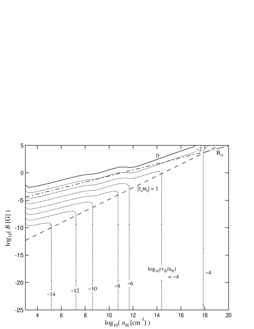
Figure 9: Same as Figure 7 except that this model is calculated without Li.

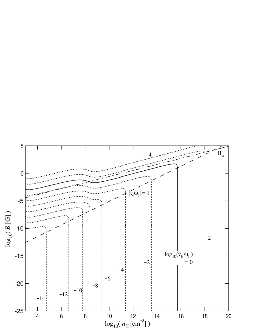
Figure 10: Same as Figure 8 except that this model is calculated without Li.

References

- Abel, Bryan & Norman (2000) Abel, T., Bryan, G. L., & Norman, M. L. 2000, ApJ, 540, 39
- Abel, Bryan & Norman (2002) Abel, T., Bryan, G. L., & Norman, M. L. 2002, Science, 295, 93
- Becker et al. (2001) Becker, R. H. et al. 2001, AJ, 122, 2850
- Bodenheimer et al. (2000) Bodenheimer, P., Burkert, A., Klein, R., & Boss, A. P. 2000, Protostars and Planets IV 2000, eds. V. Mannings, A. P. Boss, and S. S. Russel, U. of Arizona Press, 675
- Bromm, Coppi & Larson (1999) Bromm, V., Coppi, P. S., & Larson, R. B. 1999, ApJ, 527, L5
- Bromm, Coppi & Larson (2002) Bromm, V., Coppi, P. S., & Larson, R. B. 2002, ApJ, 564, 23
- Carlberg (1981) Carlberg, R. G. 1981, MNRAS, 197, 1021,
- Fan et al. (2002) Fan, X. et al. 2002, AJ, 123, 1247
- Flower (2002) Flower, D. R. 2002, MNRAS, 333, 763
- Galli & Palla (1998) Galli, D., & Palla, F. 1998, A&A, 335, 403
- Hawley & Balbus (1992) Hawley, J. F., & Balbus, S. A. 1992, ApJ, 400, 595
- Hayashi (1981) Hayashi, M. 1981, Inst. Plasma Phys. Japan Int. Rep. IPPJ-AM-19
- Hutchins (1976) Hutchins, J. B. 1976, ApJ, 205, 103
- Kamaya & Nishi (2000) Kamaya, H., & Nishi, R. 2000, ApJ, 543, 257
- Kim & Diamond (2002) Kim, E., & Diamond, P. H. 2002, ApJ, 578, L113
- Kogut et al. (2003) Kogut, A. et al. 2003, ApJS, 148, 161
- Kulsrud et al. (1997) Kulsrud, R. M., Cen, R., Ostriker, J. P., & Ryu, D. 1997, ApJ, 480, 481
- Langer, Puget & Aghanim (2003) Langer, M., Puget, J., & Aghanim, N. 2003, Phys. Rev. D, 67, 43505
- Larson (1969) Larson, R. 1969, MNRAS, 145, 271
- Lepp, Stancil & Dalgarno (2002) Lepp, S., Stancil, P. C., & Dalgarno, A. 2002, J. Phys. B, 35, R57
- Ma (2002) Ma, F. 2002, MNRAS, 335, L99
- Matsuda, Sato & Takeda (1969) Matsuda, T., Sato, H., & Takeda, H. 1969, Prog. Theor. Phys., 42, 219
- Nakamura & Umemura (1999) Nakamura, F., & Umemura, M. 1999, ApJ, 515, 239
- Nakamura & Umemura (2001) Nakamura, F., & Umemura, M. 2001, ApJ, 548, 19
- Nakamura & Umemura (2002) Nakamura, F., & Umemura, M. 2002, ApJ, 569, 549
- Nakano & Umebayashi (1986) Nakano, T., & Umebayashi, T. 1986, MNRAS, 218, 663
- Omukai (2000) Omukai, K. 2000, ApJ, 534, 809
- Omukai & Nishi (1998) Omukai, K., & Nishi, R. 1998, ApJ, 508, 141
- Oh (2002) Oh, S. P. 2002, MNRAS, 336, 1021
- Osterbrock (1961) Osterbrock, D. E. 1961, ApJ, 134, 270
- Palla, Salpeter & Stahler (1983) Palla, F., Salpeter, E. E., & Stahler, S. W. 1983, ApJ, 271, 632
- Penston (1969) Penston, M. V. 1969, MNRAS, 144, 425
- Pudritz & Silk (1989) Pudritz, R. E., & Silk, J. 1989, ApJ, 342, 650
- Puy & Signore (1996) Puy, D., & Signore, M. 1996, A&A, 305, 371
- Sano, Inutsuka & Miyama (1998) Sano, T., Inutsuka, S., & Miyama, S. M. 1998, ApJ, 506, L57
- Sano, Miyama, Umebayashi, & Nakano (2000) Sano, T., Miyama, S. M., Umebayashi, T., & Nakano, T. 2000, ApJ, 543, 486
- Sano & Inutsuka (2001) Sano, T., & Inutsuka, S. 2001, ApJ, 561, L179
- Songaila (2001) Songaila, A. 2001, ApJ, 561, L153
- Sokasian et al. (2003) Sokasian, A., Yoshida, N., Abel, T., Hernquist, L., & Springel, V. 2003, preprint, astro-ph/0307451
- Spitzer (1978) Spitzer, L. 1978, Physical Processes in the Interstellar Medium, (New York: Wiley Interscience) p.107
- Stancil, Lepp & Dalgarno (1998) Stancil, P. C., Lepp, S., & Dalgarno, A. 1998, ApJ, 509, 1
- Stone et al. (2000) Stone, J., Gammie, C., Balbus, S., & Hawley, J. Protostars and Planets IV 2000, eds. V. Mannings, A. P. Boss, and S. S. Russel, U. of Arizona Press, 589
- Susa, Uehara & Nishi (1996) Susa, H., Uehara, H., & Nishi, R. 1996, Prog. Theor. Phys., 96, 1073
- Susa et al. (1998) Susa, H., Uehara, H., Nishi, R., & Yamada, M. 1998, Prog. Theor. Phys., 100, 63
- Tan & Blackman (2004) Tan, J. C., & Blackman, E. G. 2004, accepted to ApJ, astro-ph/0307455
- Tan & McKee (2004) Tan, J. C., & McKee, C. F. 2004, accepted to ApJ, astro-ph/0307414
- Uehara et al. (1996) Uehara, H., Susa, H., Nishi, R., Yamada, M., & Nakamura T. 1996, ApJ, 473, L95
- Uehara & Inutsuka (2000) Uehara, H., & Inutsuka, S. 2000, ApJ, 531, L91
- Vladilo (2002) Vladilo, G. 2002, A&A, 391, 407
- White et al. (2003) White, R. L., Becker, R. H., Fan, X., & Strauss, M. A. 2003, AJ, 126, 1
- Widrow (2002) Widrow, L. M. 2002, Rev. Mod. Phys., 74, 775