Electron Acceleration around the Supermassive Black Hole at the Galactic Center

Abstract

The recent detection of variable infrared emission from Sagittarius A*, combined with its previously observed flare activity in X-rays, provides compelling evidence that at least a portion of this object’s emission is produced by nonthermal electrons. We show here that acceleration of electrons by plasma wave turbulence in hot gases near the black hole’s event horizon can account both for Sagittarius A*’s mm and shorter wavelengths emission in the quiescent state, and for the infrared and X-ray flares, induced either via an enhancement of the mass accretion rate onto the black hole or by a reorganization of the magnetic field coupled to the accretion gas. The acceleration model proposed here produces distinct flare spectra that may be compared with future coordinated multi-wavelength observations. We further suggest that the diffusion of high energy electrons away from the acceleration site toward larger radii might be able to account for the observed characteristics of Sagittarius A*’s emission at cm and longer wavelengths.

1 Introduction

The observation of stellar motions within light-days of Sagittarius A*, a compact radio source at the Galactic Center (Balick & Brown, 1974), has provided compelling evidence that this source is the radiative manifestation of a $\sim$ four million solar mass black hole (Schödel et al., 2002; Ghez et al., 2003). The recently detected infrared emission and flare activity have provided an additional evidence that this source is powered by a hot gas accreting onto the black hole (Baganoff et al., 2001; Goldwurm et al., 2003; Baganoff, 2003; Porquet et al., 2003; Zhao et al., 2004; Ghez et al., 2003). The quasi-periodic near-infrared variability may be an indication that the gas flared up before spiraling into the black hole (Genzel et al., 2003). It is now generally agreed that the radio and infrared emission, and the flares, are likely produced by nonthermal high energy electrons (Liu & Melia 2001; Genzel et al. 2003; see also Mahadevan 1998). However, the exact nature of the mechanism responsible for the acceleration of the electrons has not been addressed. This has given rise to diverse interpretations of the observations with assumed spectra of the accelerated electrons (Markoff et al., 2001; Liu & Melia, 2002a; Nayakshin et al., 2003; Yuan et al., 2003).

In this letter, we show that the mechanism producing high-energy particles in solar flares works equally well in hot plasmas near the black hole. The solar flare model is based on a second order Fermi acceleration process or a stochastic acceleration (SA) of particles by interacting resonantly with plasma waves or turbulence (PWT) generated via an MHD dissipation process (see e.g. Miller & Ramaty 1987; Hamilton & Petrosian 1992; Petrosian & Liu 2004). In Sagittarius A*, nonthermal particles can be produced by the turbulence expected to be induced by the magneto-rotational instability in the accretion torus (Balbus & Hawley 1991; Melia, Liu & Coker 2001). The radiation emitted at the acceleration site can explain the quiescent state mm and shorter wavelength observations. Solar flares are energized by the process of magnetic reconnection during the dynamical evolution of the coronal magnetic field. Similar processes in Sagittarius A* can release energy in a small region and produce what we call a local event. A global flare can be induced by an MHD fluctuation in the accretion torus or an enhancement of the accretion rate onto the black hole. The emission spectra from these two energization mechanisms are quite different, and can explain the distinct flare behaviors.

In § 2, we outline the theory of SA. Its application to Sagittarius A* is presented in § 3. The main results of this letter are summarized in § 4, where we also discuss consequences of energetic electrons escaping the acceleration site. If such electrons can diffuse toward larger radii, they may account for Sagittarius A*’s emission at cm and longer wavelengths and has the potential to explain the observed linear and circular polarization characteristics, and variabilities of this source.

2 Stochastic Electron Acceleration

In the theory of SA (Petrosian & Liu, 2004), particles are accelerated from a background plasma to higher energies by interacting resonantly with PWT. The particle distribution and the consequent emission spectrum are determined by the acceleration ($D_{\rm EE}$) and scattering ($D_{\mu\mu}$) rates due to the PWT, the energy loss rate ${\dot{E}}_{\rm L}$, and the spatial diffusion time $T_{\rm esc}$. These rates and time are determined by the magnetic field $B$, density $n$ and particle distribution of the background plasma, the spectrum and intensity of the turbulence, and the size of the acceleration site $R$.

The wave modes in a plasma are described by the dispersion relation $\omega=\omega({\bf k})$, which depends primarily on the plasma parameter $\alpha=\omega_{\rm pe}/\Omega_{\rm e}=(4\pi m_{\rm e}n)^{1/2}c/B\,,$ the ratio of the electron plasma frequency $\omega_{\rm pe}=(4\pi ne^{2}/m_{\rm e})^{1/2}$ to the nonrelativistic electron gyrofrequency $\Omega_{\rm e}=eB/m_{\rm e}c$, where $m_{\rm e}$, $c$ and $e$ are the electron mass, the speed of light, and the elemental charge unit, respectively. Electrons with Lorentz factor $\gamma$, velocity $v$, and pitch angle cosine $\mu$ couple strongly with the wave satisfying the resonance condition: $\omega=k_{||}v\mu+\gamma^{-1}\,,$ where $\omega$ and $k_{||}$ are the wave frequency and wave vector parallel to the large scale magnetic field (only the first harmonic of the gyrofrequency is considered here). Electrons with higher energies resonate with waves with smaller wave numbers ($k$) corresponding to larger spatial scales.

In the following discussion, we adopt a turbulence spectrum characterized by a broken power law with a lower wavenumber cutoff at $k_{\rm min}$, corresponding to the scale where the turbulence is generated ($<R$), and a break wavenumber $k_{\rm max}$ above which the wave dissipation is fast. We will study the SA by a PWT propagating parallel to the large scale magnetic field. The characteristic interaction time $\tau_{\rm p}$ is given by $\tau_{\rm p}^{-1}=(\pi/2)\Omega_{\rm e}(8\pi{\cal E}_{\rm tot}/B^{2})(q-1)k_{\rm min}^{q-1}\,,$ where $q>1$ is the turbulence spectral index in the inertial range and ${\cal E}_{\rm tot}$ is the total turbulence energy density. Relativistic electrons interacting with waves in a plasma with $\alpha>(m_{\rm e}/m_{\rm p})^{1/2}\simeq 1/43$, where $m_{\rm p}$ is the proton mass, will have an isotropic distribution because of the short scattering time $\tau_{\rm sc}=1/D_{\mu\mu}$. In such plasmas electrons can gain energy by interacting with the waves and lose energy either via Coulomb collisions with background plasma particles (at lower energies) or by radiative processes (at higher energies). The electrons also diffuse spatially and leave the region on a characteristic time $T_{\rm esc}\sim R^{2}/\beta^{2}c^{2}\tau_{\rm sc}$. The spatially integrated electron distribution $N(E)$, as a function of the kinetic energy $E$, satisfies the well known diffusion-convection equation:

$${\partial N\over\partial t}={\partial^{2}\over\partial E^{2}}(D_{EE}N)+{\partial\over\partial E}[({\dot{E}}_{\rm L}-A)N]-{N\over T_{\rm esc}}+Q\,,$$ (1)

where $D_{EE}$ and $A$ are obtained from the wave-particle interaction rates and $Q$ is a source term. In Sagittarius A*, where the photon energy density is at least one order of magnitude lower than the magnetic field energy density, the radiative loss of relativistic electrons is dominated by synchrotron process, for which

$$\tau_{\rm loss}=E/\dot{E}_{\rm L}={\gamma-1\over 4\pi r_{\rm o}^{2}cn(\ln{\Lambda}/\beta+4\beta^{2}\gamma^{2}/9\alpha^{2})}\,,$$ (2)

where $\ln{\Lambda}\simeq 20$ and the first and second term in the denominator give the Coulomb collision and synchrotron loss rate, respectively.

3 Application to Sagittarius A*

To determine the exact turbulence spectrum, one needs to solve the coupled kinetic equations of the waves and particles and their solutions depend on the wave generation, cascade, dissipation processes and the distribution of the background particles (see e.g. Miller, LaRosa & Moore 1996). The lack of a well established theory for the MHD turbulence renders such a treatment unpractical. As an approximation, we set $k_{\rm min}=2\pi\eta/R$ with $\eta>1$, where the characteristic variation length of the large scale magnetic field $R/\eta$ is related to the turbulence generation length scale. To estimate $k_{\rm max}$, we note that the wave damping is efficient when the waves start to resonate with the background particles. From the resonance condition, one has $k_{\rm max}\sim\Omega_{\rm e}/(c<\gamma>)$, where $<\gamma>$ is the mean Lorentz factor of the background electrons, which is expected to be $\sim 50$ near the black hole of Sagittarius A*. For $k_{\rm min}\leq k\leq k_{\rm max}$ the turbulence most likely has a Kolmogorov spectrum with an index $q=5/3$ and above $k_{\rm max}$ the index changes to 4.0, a typical value obtained from MHD simulations (Hawley et al., 1995; Vestuto et al., 2003). MHD simulations (Hawley et al., 1995; Hirose et al., 2004) also suggest that the magnetic field energy density is about a few percent of the energy density of the background gas, which means that $\alpha\sim 1$ (note that $\alpha^{2}=0.5nm_{\rm e}c^{2}/[B^{2}/8\pi]$), and that ${\cal E}_{\rm tot}\lesssim B^{2}/8\pi$. The accretion flow in Sagittarius A* is collisionless; it is not clear how the particle distribution of the accretion plasma evolves from large to small radii, where it enters the acceleration site of strong dissipation and PWT. We make the reasonable assumption that the source electrons have a relativistic Maxwellian distribution. We therefore have ${\cal E}_{\rm tot}=ank_{\rm b}T$ with $a\ll 1$ as a model parameter. The exact spatial diffusion time (or $T_{\rm esc}$) depends on the structure of the magnetic field (Hirose et al., 2004) and the scattering rate. We set $T_{\rm esc}=\tau_{\rm tr}^{2}/\tau_{\rm sc}+\tau_{\rm tr}$, where the transit time $\tau_{\rm tr}=\eta R/v$ determines the escape time when the scattering time $\tau_{\rm sc}\gg\tau_{\rm tr}$ (Petrosian & Donaghy, 1999; Petrosian & Liu, 2004).

During big flares, the physical conditions are expected to undergo dramatic changes, which may affect the turbulence spectrum and the energy partition among the gas, turbulence, and magnetic field. These processes are not well understood. For the purpose of illustration, we will make the following reasonable assumption to reduce the number of parameters. We set $\eta=2$, $k_{\rm max}=0.02\,\Omega_{\rm e}/c=1.2\times 10^{-5}(B/G)$ cm^-1, $\alpha=1$ and $a=0.008$. This leaves only three independent parameters; here we choose $R$, $n$ and $\tau_{\rm p}$. All other quantities can be derived from them.

To calculate the emission predicted by the model, one also needs to specify the geometry of the source. We will assume that the source is uniform and spherically symmetric with a radius $R$, which may or may not be centered on the black hole. (Note that although the actual geometry is inferred to be Keplerian for a global acceleration region—see, e.g., Melia et al. 2001a—its differences from the simplified geometry adopted here are expected to change the required model parameters only slightly. This is a fair assumption for local fluctuations.) For flares induced by an enhanced accretion rate, the density $n$ can increase dramatically while $R$ and $\tau_{\rm p}$ may not change much at all. For local MHD fluctuations, all three parameters can experience significant changes (Hawley et al., 1995).

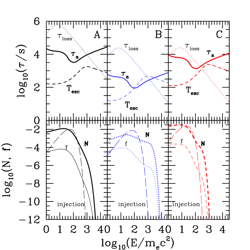
Figure 1: Top Panels: The time scale for acceleration $\tau_{\rm a}=E/A$ (solid lines), escape (dashed lines) and loss $\tau_{\rm loss}=E/\dot{E}_{\rm L}$ (dotted lines) for Models A (left panel), B (middle panel) and C (right panel). The model parameters are given in Table 1. The loss term is dominated by Coulomb collisions below the peak and by synchrotron losses above it. Bottom Panels: The normalized electron distributions N (thick lines) at the acceleration site and the corresponding escape fluxes $f=N/T_{\rm esc}$ (thin lines). The long dashed lines show the source Maxwellian electron distribution. See text for details.

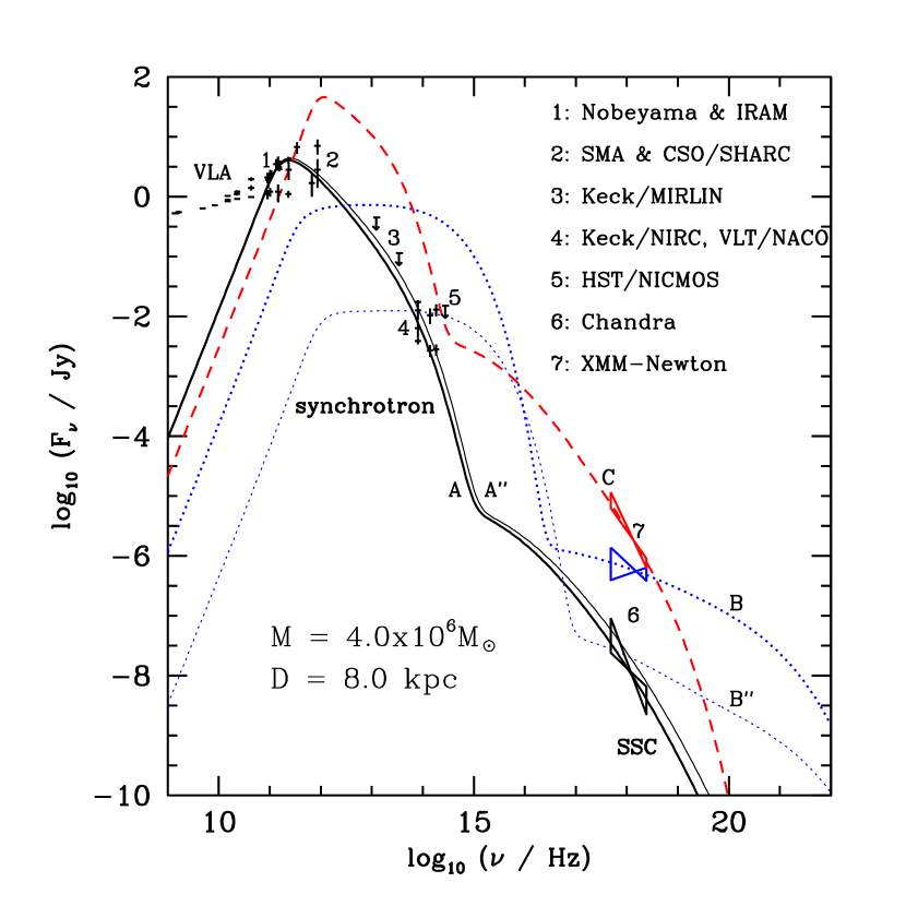
Figure 2: Model fits to the broadband spectrum of Sagittarius A*. The data are gathered from observations made at different epochs (the instruments are indicated in the figure by the numbers). In the radio and infrared bands, the upper set of data show Sagittarius A*’s peak flux densities during the brightest flares observed so far, while at the same frequencies, the lower data points correspond to its emission in the quiescent state. The middle set of data in the radio are the averaged flux densities. The upper butterfly in the X-ray band gives the peak flux density for the flare observed by XMM-Newton on October 3 2002. The middle one gives the peak flux density for the 10-27-2000 flare observed by Chandra. The lower one corresponds to the averaged X-ray emission in the quiescent state. The upper limits are also for the quiescent state emission. The spectrum produced by each of the five models in Table 1 is indicated by a continuous curve. See text and the caption of Table 1 for details of the models.

In Table 1, we summarize parameters of several models that account for Sagittarius A*’s spectrum in its various states (Figure 2). The corresponding time scales and normalized electron distributions in the steady state are shown in Figure 1 for Models A (left panel), B (middle panel) and C (right panel). The valleys in the acceleration and the peaks in the escape time correspond to the spectral break $k_{\rm max}$ of the turbulence. The loss time $\tau_{\rm loss}\equiv E/\dot{E}_{\rm L}$ peaks at an energy, which only depends on the plasma parameter $\alpha$ (see eq. [2]). In the lower panels of the figure, we also show the source thermal electron distribution and the flux $f=N/T_{\rm esc}$ of escaping electrons. It is crucial to note that the acceleration time for Model B (Model C) is shorter than the duration of X-ray flares with a hard (soft) spectrum. We can therefore use the steady state electron distribution to calculate the synchrotron and synchrotron self-Comptonization (SSC) photon spectra of the models. These are compared with Sagittarius A*’s spectra in its various states in Figure 2, where the data are gathered from observations made at different epochs (Falcke et al., 1998; Zhao et al., 2003; Miyazaki et al., 1999, 2003; Serabyn et al., 1997; Dowell, 2003; Cotera et al., 1999; Stolovy et al., 2003; Baganoff et al., 2003).

Model A explains Sagittarius A*’s emission at frequencies above $100$ GHz in the quiescent state. The mm to infrared emission is produced via synchrotron processes, whereas the optical to gamma-ray emission is produced by SSC (see Melia et al. 2000). Global fluctuations in the PWT will vary $\tau_{\rm p}$ and result in a different spectrum. For example, by increasing $\tau_{\rm p}^{-1}$ by $5\%$, we obtain Model A^′′, which predicts a weak flare with a soft spectrum. The flux densities in the infrared and X-ray bands increase by $\sim 80\%$. Such a flare is clearly detectable in the infrared by VLT and Keck, but not by the existing X-ray instruments due to its low flux. If the flare only lasted for a few hours, neither Chandra nor XMM-Newton would be able to detect it. Actually, Sagittarius A*’s quiescent state X-ray spectrum is obtained by averaging over a long observation period (Baganoff et al., 2003), which will smooth out contribution from such weak flares. This aspect of the model therefore may explain why the occurrence frequency of infrared flares is more than twice that of X-ray flares (Genzel et al., 2003).

Model B (B^′′) reproduces X-ray (and probably infrared) flares with hard spectra. Compared with Model A (A^′′), it has a much smaller radius, which suggests that this is a localized (as opposed to global) event. The quiescent state emission of Model A presumably still exists during this type of flare. If the plasma is in a Keplerian motion (see Melia et al. 2001), one would expect to detect quasi-periodic variability, as has been seen in the infrared (Genzel et al., 2003), and apparently now in X-rays as well (Aschenbach et al. 2004). Note that in the energy range $80\lesssim\gamma\lesssim 2000$ the acceleration time is shorter than the escape time (middle panel of Figure 1). This means that the acceleration of electrons in this range is more efficient than at lower energies, resulting in a harder electron distribution and corresponding harder photon spectrum. These spectra are cut off sharply where $\tau_{\rm loss},T_{\rm esc}<\tau_{\rm a}$. Such flares are likely produced by a local fluctuation (possibly a reconfiguration or reconnection of the magnetic field), which produces strong PWT, trapping electrons within the acceleration site more efficiently. This model explains the 10-27-2000 flare observed by Chandra and predicts strong infrared emission accompanying the X-ray flare. Model B^′′ is obtained by decreasing $R$ by a factor of $13$ while keeping $nR\propto(\tau_{\rm a}T_{\rm esc})^{1/2}/\tau_{\rm loss}$ and $R/\tau_{\rm p}\propto(T_{\rm esc}/\tau_{\rm a})^{1/2}$ the same as in Model B, so that the spectrum does not change significantly. This model predicts weaker infrared and X-ray flares, but the spectra are harder, which may explain the weak X-ray flares observed by Chandra (Baganoff, 2003), and the recently observed infrared flares (Genzel et al., 2003; Ghez et al., 2003).

In Model C, which explains the 10-3-1002 XMM-Newton flare, the synchrotron loss dominates at very low energy ($\gamma\sim 200$). The corresponding electron distribution and X-ray spectrum are steeper. Given the required high density and large volume for this model, this type of event is likely induced by an enhancement of the accretion rate onto the black hole. Future multi-wavelength observations will be able to test the high flux of sub-mm and IR radiation predicted by this model.

4 Summary and Discussions

Based on the theory of stochastic particle acceleration, we have built a model to account for Sagittarius A*’s emission at mm and shorter wavelengths. The quiescent state emission is attributed to electrons accelerated by turbulence in a magnetized accretion torus and flares can be produced via two distinct mechanisms. The IR and X-ray flares with harder spectrum are likely induced by a local MHD process, such as magnetic reconnection. Global fluctuations generally produce flares with IR and X-ray spectral indexes close to their corresponding value in the quiescent state. The model not only accounts for the varied spectra of the flares, but also explains their relative occurrence rate observed at IR and X-ray.

Radio emission at longer wavelengths cannot be produced within such a small emission region (Liu & Melia, 2001). This is not surprising, given that the radio emission is variable on a longer time scale of tens of hours to one week, suggesting that this radiation is produced at larger radii than what we have been considering here (Zhao et al., 2004, 2003; Zhao & Goss, 1993; Bower et al., 2002). Very interestingly, our model suggests a significant outflow of high-energy electrons (Liu & Melia, 2002b), which may very well be the particles that eventually produce Sagittarius A*’s cm spectrum via synchrotron emission on a spatially larger scale. In the quiescent state (Model A), the power carried away by electrons with $\gamma>100$ (electrons with lower energy may be trapped by the gravitational potential of the black hole and will not diffuse to larger radii) is about $2\times 10^{37}$ ergs s^-1, which is more than enough to power the observed radio emission, whose luminosity is about $10^{34-35}$ ergs s^-1. (Note that in this model, the mass accretion rate is $\sim 10^{18-19}$g s^-1, for which a few percent of the dissipated gravitational energy is carried away by the outwardly diffusing electrons; see the caption of Table 1.) For the XMM-Newton flare on October 3 2002 (Model C), the total energy carried away by the escaping high-energy electrons is about $7\times 10^{40}$ ergs which for a few days can sustain the radio flare observed 13 hours after the X-ray event (Zhao et al., 2004). This picture also explains the weak correlation between the Chandra X-ray flares and the radio emission from Sagittarius A* (Baganoff, 2003), because the flux of high energy electrons produced during these flares is much smaller than that for the XMM-Newton flare; no strong enhancement of radio emission is expected following a Chandra-type of X-ray flare.

One of the intriguing properties of Sagittarius A*’s radio emission is that it is circularly polarized below $100$ GHz, even though no linear polarization has been observed there (Bower et al., 2002). However, in the mm and sub-mm range only strong linear polarization is observed (Aitken et al., 2000; Bower et al., 2003). The mm/sub-mm polarization is likely associated with the structure of the magnetic field at small radii (Agol, 2000; Melia et al., 2000; Bromley et al., 2001), which is consistent with the spectral formation at these wavelengths discussed in this paper. The observed circular polarization may be due to anisotropy of the escaping electrons as they are transported along magnetic field lines toward larger radii under the influence of synchrotron losses (McTiernan & Petrosian, 1990). Relativistic electrons beamed along magnetic field lines produces synchrotron emission with significant circular polarization while the degree of linear polarization can be suppressed by irregularities in the source magnetic field (Epstein, 1973; Epstein & Petrosian, 1973). Work to demonstrate this feature self-consistently is in progress, and the results will be reported elsewhere. The model we have presented here shows promise in being able to account not only for the spectral characteristics of Sagittarius A*, but also for its polarization characteristics and time variation properties.

Finally, we emphasize that although we suggested that $\eta$, $k_{\rm max}/\Omega_{\rm e}$, $\alpha$, and $a$ may not change significantly over time, and have fixed them in all the models discussed above, given the dramatic changes of the physical conditions during a flare state, these parameters may also vary slightly, giving rise to different emission spectra than those presented here. Indeed, if the infrared upper limits reported by Hornstein et al. (2002) are confirmed, one then needs to decrease the high frequency cutoff of the synchrotron emission by adjusting these parameters. This will be investigated in a more comprehensive study of particle acceleration in Sagittarius A*.

Table 1: Models and Parameters.

Models	$R$($r_{S}$)	$\tau_{\rm p}^{-1}$ (s-1)	$n$ ($10^{7}$cm-3)	$B$ (Gauss)	$k_{\rm b}T$ ($m_{\rm e}c^{2}$)	$Q$ ($10^{42}$s-1)
A (A′′)	2.5	0.74 (0.78)	0.76	8.8	26.0 (27.3)	3.2 (3.0)
B (B′′)	0.22 (0.017)	26.7 (345)	19.0 (240)	44 (160)	34.2 (20.5)	0.11 (0.014)
C	1.9	1.78	18.0	43	10.5	49

References

- Agol (2000) Agol, E. 2000, ApJ, 538, L121
- Aitken et al. (2000) Aitken, D. et al. 2000, ApJ, 534, L173
- Aschenbach et al. (2004) Aschenbach, B. et al. 2004, A&A, in press
- Baganoff et al. (2001) Baganoff, F. K. et al. 2001, Nature, 413, 45
- Baganoff (2003) Baganoff, F. K. 2003, (HEAD) AAS Abstr. 3.02, 35
- Baganoff et al. (2003) Baganoff, F. K. et al. 2003, ApJ, 591, 891
- Balbus & Hawley (1991) Balbus, S. A., & Hawley, J. F. 1991, ApJ, 376, 214
- Balick & Brown (1974) Balick, B., & Brown, R. L. 1974, ApJ, 194, 265
- Bower et al. (2002) Bower, G. C., Falcke, H., Sault, R. J., & Backer, D. C. 2002, ApJ, 571, 843
- Bower et al. (2003) Bower, G. C. Wright, Melvyn C. H. Falcke, H., & Backer, D. C. 2003, ApJ, 588, 331
- Bromley et al. (2001) Bromley, B., Melia, F., and Liu, S. 2001, ApJ, 555, L83
- Cotera et al. (1999) Cotera, A. et al. 1999, ASP Conf. Ser., 186, 240
- Dowell (2003) Dowell, C. D. 2003, private communication
- Epstein (1973) Epstein, R. I. 1973, ApJ, 183, 593
- Epstein & Petrosian (1973) Epstein, R. I., & Petrosian, V. 1973, ApJ, 183, 611
- Falcke et al. (1998) Falcke, H. et al. 1998, ApJ, 499, 731
- Hirose et al. (2004) Hirose, S., Krolik, J. H., De Villiers, J. P., & Hawley, J. F. 2004, ApJ, in the press.
- Genzel et al. (2003) Genzel R. et al. 2003, Nature, 425, 934
- Ghez et al. (2003) Ghez, A. M. et al. 2003, ApJ, (submitted)
- Ghez et al. (2003) Ghez, A. M. et al. 2003, ApJ, (submitted); preprint at astro-ph/0306127
- Goldwurm et al. (2003) Goldwurm, A. et al. 2003, ApJ, 584, 751
- Hamilton & Petrosian (1992) Hamilton, R. J., & Petrosian, V. 1992, ApJ, 398, 350
- Hawley et al. (1995) Hawley, J. F., Gammie, C. F., & Balbus, S. A. 1995, ApJ, 440, 742
- Hornstein et al. (2002) Hornstein, S. D. et al. 2002, ApJ, 577, L9
- Liu & Melia (2001) Liu, S., & Melia, F. 2001, ApJ, 561, L77
- Liu & Melia (2002a) Liu, S., & Melia, F. 2002a, ApJ, 566 L77
- Liu & Melia (2002b) Liu, S., & Melia, F. 2002b, ApJ, 573, L23
- Mahadevan (1998) Mahadevan, R. 1998, Nature, 394, 651
- Markoff et al. (2001) Markoff, S., Falcke, H., Yuan, F., & Biermann, P. L. 2001, AJ, 379, L13
- McTiernan & Petrosian (1990) McTiernan, J. M., & Petrosian, V. 1990, ApJ, 524
- Melia et al. (2000) Melia, F., Liu, S., & Coker, R. 2000 ApJ, 545, L117
- Melia et al. (2001) Melia, F., Liu, S., & Coker, R. 2001, ApJ, 553, 146
- Miller, LaRosa, & Moore (1996) Miller, J., LaRosa, T. N., & Moore, R. L. 1996, ApJ, 461, 445
- Miller & Ramaty (1987) Miller, J., & Ramaty, R. 1987, Solar Physics 113, 195
- Miyazaki et al. (1999) Miyazaki, A., Tsutsumi, T., & Tsuboi, M. 1999, Adv. Space Res., 23, 977
- Miyazaki et al. (2003) Miyazaki, A., Tsutsumi, T., & Tsuboi, M. 2003, Astron. Nachr. 324, S1, 363
- Nayakshin et al. (2003) Nayakshin, S., Cuadra, J., & Sunyaev, R. 2003, A&A, 413, 173
- Petrosian & Donaghy (1999) Petrosian, V., & Donaghy, T. 1999, ApJ, 527, 945
- Petrosian & Liu (2004) Petrosian, V., & Liu, S. 2004, ApJ, (submitted); preprint at astro-ph/0401585
- Porquet et al. (2003) Porquet, D. et al. 2003, A&A, 413, L17
- Schödel et al. (2002) Schödel, R. et al. 2002, Nature, 419, 694
- Serabyn et al. (1997) Serabyn, E. et al. 1997, ApJ, 490, L77
- Stolovy et al. (2003) Stolovy, S., Melia, F., McCarthy, D., & Yusef-Zadeh, F. 2003, Astron. Nachr., 324, S1, 419
- Vestuto et al. (2003) Vestuto, J. G., Ostriker, E. C., & Stone, J. M. 2003, ApJ, 590, 858
- Yuan et al. (2003) Yuan, F., Quataert, E., & Narayan, R. 2003, ApJ, 598, 301
- Zhao et al. (2004) Zhao, J. H., Herrnstein, R. M., Bower, G. C., Goss, W. M., & Liu, S. 2004, ApJ, 603, L85
- Zhao et al. (2003) Zhao, J. H. et al. 2003, ApJ, 586, L29
- Zhao & Goss (1993) Zhao, J. H., & Goss, W. M. 1993, Sub-arcsecond radio astronomy (Cambridge: Cambridge Univ. Press), 38