Extragalactic UHE proton spectrum and prediction for iron-nuclei flux at $10^{8}-10^{9}$ GeV

Abstract

We investigate the problem of transition from galactic cosmic rays to extragalactic ultra high energy cosmic rays. Using the model for extragalactic ultra high energy cosmic rays and observed all-particle cosmic ray spectrum, we calculate the galactic spectrum of iron nuclei in the energy range $10^{8}-10^{9}$ GeV. The flux and spectrum predicted at lower energies agree well with the KASCADE data. The transition from galactic to extragalactic cosmic rays is distinctly seen in spectra of protons and iron nuclei, when they are measured separately. The shape of the predicted iron spectrum agrees with the Hall diffusion.

, ,

1 Introduction

There are now convincing evidences that ultra high energy cosmic rays (UHECR) in the energy range $1\times 10^{18}-8\times 10^{19}$ eV are extragalactic protons. These evidences include: (i) Measurement by HiRes detector [1] of $x_{\rm max}$ in EAS longitudinal development favours protons as primaries at $E\geq 1\times 10^{18}$ eV (see Fig. 1), (ii) The energy spectra measured by Akeno-AGASA [2], Fly’s Eye [3], HiRes [4] and Yakutsk [5] detectors clearly show the dip [6] (see Fig.2) , which is a signature of interaction of extragalactic protons with CMB radiation, (iii) The beginning of the GZK cutoff up to $E\approx 8\times 10^{19}$ eV is seen in all data, including that of AGASA (see Fig. 2).

Figure 1: The HiRes data [1] on mass composition (preliminary). The measured $x_{\rm max}$ at $E\geq 1\times 10^{18}$ eV are in a good agreement with QGSJet-Corsika prediction for protons.

It is interesting to note that the excess, detected by AGASA [7] at $E\sim 10^{18}$ eV from directions to the galactic sources, Galactic Center and Cygnus, may be naturally interpreted as evidence of diffuse extragalactic flux at $E\geq 1\times 10^{18}$ eV. Indeed, if transition from galactic to extragalactic diffuse flux occurs due to failure of magnetic confinement in the Galaxy, the unconfined flux from the galactic sources should become visible above energy of the transition.

On the other hand, not all experimental data agree with pure proton composition at $E\geq 1\times 10^{18}$ eV. While data of HiRes-MIA[8] and Yakutsk [9] support such composition, the data of other detectors, such as Fly’s Eye [10], Haverah Park [11] and Akeno [12] favour the mixed composition at $E\geq 1\times 10^{18}$ eV. The indirect confirmation of the proton composition at $E\geq 1\times 10^{18}$ eV comes from the KASCADE data [13], which show disappearance of the heavy nuclei from the CR flux at much lower energies.

UHECR have a problem with the highest energy events. First of all, 11 AGASA events at $E\geq 1\times 10^{20}$ eV comprise significant excess (not seen by HiRes) over predicted flux (see Fig. 2). This excess may be interpreted as the new component of UHECR, probably due to one of the top-down scenarios (see [14]). Even if to exclude the AGASA data from analysis, the problem with particles at $E>1\times 10^{20}$ eV remains. There are three events with $E>1\times 10^{20}$ eV observed by other detectors, namely, one Fly’s Eye event with $E\approx 3\times 10^{20}$ eV, one HiRes event with $E\approx 1.8\times 10^{20}$ eV and one Yakutsk event with $E\approx 1.0\times 10^{20}$ eV. The attenuation length of protons with energies $(2-3)\times 10^{20}$ eV is only 20 - 30 Mpc. With correlations of UHECR directions with AGN (BL Lacs) observed at $(4-8)\times 10^{19}$ eV [15], the AGN must be observed in the direction of these particles. If to exclude the correlations with AGN from analysis, the propagation in the strong magnetic fields becomes feasible [16]. Nevertheless, also in this case the lack of the nearby sources in the direction of highest energy events (e. g. at $E\sim 3\times 10^{20}$ eV) remains a problem for reasonable local field $H\sim 1$ nG. Indeed, the deflection angle $\theta\sim l_{\rm att}/r_{H}=3.7^{\circ}H_{\rm nG}$ is small, and the source should be seen within this angle.

Figure 2: Comparison of calculated spectra for non-evolutionary model (see the text) with observational data. There is a good agreement of a dip centered at $E\sim 1\times 10^{19}$ eV with all data. The dip is produced due to pair-production $p+\gamma_{\rm CMB}\to p+e^{+}+e^{-}$ on CMB radiation. AGASA excess needs for its explanation another component of UHECR (shown by dashed curve), which can be due to one of the top-down scenarios [14].

Another problem with UHECR exists at its low energy edge. The transition from galactic to extragalactic cosmic rays may occur at position of the second knee. The energy of the second knee varies from $4\times 10^{17}$ eV to $8\times 10^{17}$ eV in different experiments (Fly’s Eye – $4\times 10^{17}$ eV [3], Akeno – $6\times 10^{17}$ eV [17], HiRes – $7\times 10^{17}$ eV [4] and Yakutsk – $8\times 10^{17}$ eV [5]). This energy is close to $E\sim 1\times 10^{18}$ eV, where according to the HiRes data [8] protons start to dominate the flux. On the other hand, KASCADE data [13] show disappearance of galactic cosmic rays at much lower energy. In Fig. 3 one can see that positions of the proton, helium, carbon and iron knees can be tentatively accepted as $2.5\times 10^{15}$ eV,  $5.5\times 10^{15}$ eV,  $1.8\times 10^{16}$ eV,  and $7.0\times 10^{16}$ eV, respectively (see arrows in Fig. 3).

How the gap between the knee for iron nuclei and the beginning of the extragalactic component is filled? Why the transition reveals itself in the form of hardly noticeable feature in all-particle spectrum?

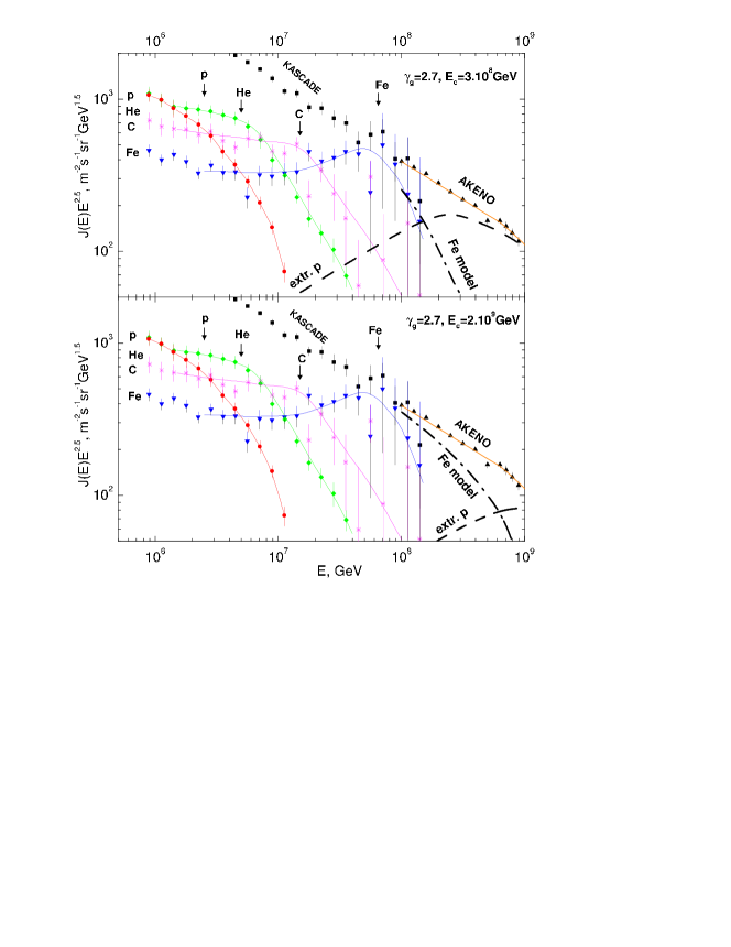
Figure 3: The calculated spectra of extragalactic protons (thick dashed curve labeled “extr. p”) and of galactic iron nuclei (dash-dotted thick curve labeled “Fe model”) in comparison with the Akeno and KASCADE data. The values of $\gamma_{g}$ and $E_{c}$ used in the calculations are indicated in each panel. The all-particle spectrum of Akeno is shown by filled triangles and by solid curve. The sum of the curves “extr. p” and “Fe model” is exactly equal to all-particle spectrum of Akeno, given by curve “AKENO”. The data of KASCADE for different nuclei are shown as : protons – by filled circles, helium – by diamonds, carbon – by stars, and iron – by inverted triangles. The thin full curves smoothly connect the data points. The arrows labeled by p, He, C and Fe show the positions of corresponding knees, calculated as $E_{Z}=ZE_{p}$, with $E_{p}=2.5\times 10^{6}$ GeV. One can notice the satisfactory agreement between calculated and observed positions of the knees.

2 The model

We will construct here the phenomenological model, which predicts the spectrum of iron nuclei in the energy range $8\times 10^{7}-1\times 10^{9}$ GeV. Following Ref. [6], we will calculate the spectrum of extragalactic protons in the energy range $10^{8}-10^{12}$ GeV. Subtracting this proton spectrum from the observed all-particle spectrum (we shall use Akeno-AGASA data), we obtain residual spectrum, which, inspired by the KASCADE data, we assume to be comprised by iron nuclei. This spectrum will be compared with that measured by KASCADE. The justification of this model consists in confirmation of the dip in the calculated proton spectrum by observations. One of the results is description of transition from galactic to extragalactic cosmic rays. The predicted physical quantity is the flux of iron nuclei and their spectrum at $10^{8}-10^{9}$ GeV.

2.1 Spectrum of extragalactic protons

We will calculate the extragalactic proton spectrum, following Ref. [6], in the model with the following assumptions.

We assume the generation spectrum of a source

$$Q_{g}(E_{g},z)=\frac{L_{p}(z)}{\ln\frac{E_{c}}{E_{\rm min}}+\frac{1}{\gamma_{g}-2}}q_{\rm gen}(E_{g}),$$ (1)

with

$$q_{\rm gen}(E_{g})=\left\{\begin{array}[]{ll}1/E_{g}^{2}{}&{\rm at}~{}~{}E_{g}\leq E_{c}\\ E_{c}^{-2}(E_{g}/E_{c})^{-\gamma_{g}}{}&{\rm at}~{}~{}E_{g}\geq E_{c}\end{array}\right.$$ (2)

The diffuse spectrum is calculated as

$$J_{p}(E)=\frac{c}{4\pi}~{}\frac{{\mathcal{L}}_{0}}{\ln\frac{E_{c}}{E_{min}}+\frac{1}{\gamma_{g}-2}}\int_{0}^{z_{max}}dtq_{\rm gen}\left(E_{g}(E,z),E\right)\frac{dE_{g}}{dE},$$ (3)

where ${\mathcal{L}}_{0}=n_{s}L_{p}$ is emissivity (with $n_{p}$ and $L_{p}$ being the comoving density of the sources and luminosity, respectively), $E_{g}(E,z)$ is generation energy of a proton at epoch $z$, $dE_{g}/dE$ is given in Refs. [18, 19] as

$$\frac{dE_{g}(z_{g})}{dE}=(1+z_{g})exp\left\{\frac{1}{H_{0}}\int_{0}^{z_{g}}dz\frac{(1+z)^{2}}{\sqrt{\Omega_{m}(1+z)^{3}+\Omega_{\Lambda}}}\left(\frac{db_{0}(E^{\prime})}{dE^{\prime}}\right)_{E^{\prime}=(1+z)E_{g}(E,z)}\right\},$$ (4)

where $b_{0}(E)$ is the proton energy loss $dE/dt$ at $z=0$, and $dt$ is given as

$$dt=\frac{dz}{H_{0}(1+z)\sqrt{\Omega_{m}(1+z)^{3}+\Omega_{\Lambda}}},$$ (5)

with $H_{0},\Omega_{m},$ and $\Omega_{\Lambda}$ being the Hubble constant, relative cosmological density of matter and that of vacuum energy, respectively.

In calculation of the flux according to Eq. (3) we use the non-evolutionary model, taking ${\mathcal{L}}_{0}$ not dependent on redshift $z$. Since we are interested in energies $E\geq 1\times 10^{8}$ GeV the maximum redshift appears in Eq. (3) automatically due to sharp increase of $E_{g}(z)$ at large $z$. The control calculations with $z_{\rm max}=4$ give the the identical results. Notice that in evolutionary models the calculated flux is sensitive to $z_{\rm max}$.

The calculated spectrum is displayed in Fig. 2 with $E_{c}=1\times 10^{9}$ GeV and $\gamma_{g}=2.7$ in comparison with observational data. In the further calculations we fix $\gamma_{g}=2.7$ as the best fit to the observational data displayed in Fig. 2 and consider $E_{c}$ as a free parameter.

2.2 Galactic iron spectrum and transition from galactic to extragalactic cosmic rays

In Fig. 4 we show the iron galactic spectrum found as subtraction of the extragalactic proton spectrum calculated above, from all-particle spectrum (Akeno-AGASA). The transition from galactic to extragalactic cosmic rays occurs at crossing of proton and iron spectra, which is very noticeable and occurs at energies $1.5\times 10^{8}$ GeV, $3.6\times 10^{8}$ GeV and $6.2\times 10^{8}$ GeV for the curves 1-$1^{\prime}$,  2 - $2^{\prime}$  and 3 - $3^{\prime}$, respectively.

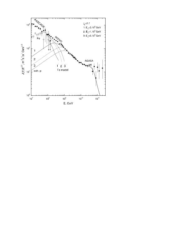
Figure 4: Calculated spectrum of extragalactic protons (curves $1,~{}2,~{}3$) and of galactic iron spectra (curves $1^{\prime},2^{\prime},3^{\prime}$) compared with all-particle spectrum from Akeno and AGASA experiments. The galactic iron spectrum is obtained by subtraction of the calculated proton spectrum from the all-particle spectrum. The pairs of curves $1$ and $1^{\prime}$, $2$ and $2^{\prime}$, $3$ and $3^{\prime}$ correspond to $E_{c}$ equal to $3\times 10^{8}$ GeV, $1\times 10^{9}$ GeV, and $2\times 10^{9}$ GeV, respectively. The intersections of the curves $1-1^{\prime}$, $2-2^{\prime}$ and $3-3^{\prime}$ give the transition from galactic (iron) to extragalactic (protons) components, which occurs at $1.5\times 10^{8}$ GeV,  $3.6\times 10^{8}$ GeV and $6.2\times 10^{8}$ GeV, respectively. The KASCADE data are shown by filled squares for all-particle fluxes and by open circles - for iron nuclei fluxes.

In Fig. 5 the fraction of iron nuclei in the total flux is shown as function of energy. Notice, that in our model in energy range $(1-10)\times 10^{8}$ GeV the total flux is comprised only by protons and iron. The Haverah Park data [11] confirm that it can be the case. The analysis of the Haverah Park data has been performed for energy-independent composition, however comparison of the obtained composition (34% of protons and 66% of iron) with our average value favours large $E_{c}$.

Figure 5: Fraction of iron nuclei in the total flux as function of energy.

The flux of iron nuclei calculated here fit well the KASCADE data at energy $E\sim 10^{8}$ GeV and below (see Fig. 3).

Why there is no pronounced feature in the total spectrum which corresponds to transition from galactic to extragalactic component? Such feature is inevitably faint when both components have approximately equal spectrum exponents. This is our case: the Akeno spectrum up to $7\times 10^{7}$ GeV is characterised by $\gamma=3.0$, while at higher energies - by $\gamma=3.25$. However, one can see from Fig. 3 that intersection of extragalactic proton spectrum (“extr. p”) and galactic iron spectrum (curve “Fe-model”) is characterised by quite prominent feature. Therefore, measuring the spectra of iron and protons separately, one can observe the transition quite distinctively.

2.3 Visibility of galactic sources at $E\gtrsim 1\times 10^{9}$ GeV

We argued above that at energy $E>E_{c}\sim 1\times 10^{9}$ GeV the extragalactic flux dominates. However, as the AGASA observations show [7] at these energies the excess of events in the direction of some galactic sources is observed. We shall show in this section that visibility of galactic sources at $E>E_{c}$ is a natural prediction of our model.

If galactic sources accelerate particles to energies higher than $1\times 10^{9}$ GeV their “direct” flux can be seen, while the produced diffuse flux should be small because of short confinement time in the galaxy. If generation spectrum is dominated by protons, the “direct”flux must be seen as the protons, while the diffuse galactic flux is presented by the heaviest nuclei.

We shall argue here that galactic point sources should be observed as the extensive sources, as it occurs in the AGASA observations [7].

Propagation of the protons from the galactic sources takes place in quasi-diffusive regime with the large diffusion coefficient. The protons arrive at an observer along a trajectory in the regular galactic magnetic field, while the small-angle scattering in the random magnetic field provides the angular distribution of protons in respect with the main direction along the trajectory. Because of the large proton energy, the scattering occurs mainly on the basic scale of the turbulent (random) magnetic field $l_{c}\sim 100$ pc. The scattering angle $\theta$ corresponds to $\langle\theta^{2}\rangle=l_{c}^{2}/r_{L}^{2}$, where $r_{L}$ is the Larmor radius in the basic magnetic field. Using $\langle B_{\perp}^{2}\rangle=(2/3)\langle B^{2}\rangle$ for the field perpendicular to a particle trajectory one obtains

$$\langle\theta^{2}\rangle=\frac{2}{3}e^{2}l_{c}^{2}\langle B^{2}\rangle/E^{2},$$ (6)

where $e$ is electric charge of the proton.

After $n$ scattering in the random magnetic field the angle with respect to the direction of the regular trajectory becomes [21, 22]    $\langle\phi^{2}\rangle=\frac{1}{3}n\langle\theta^{2}\rangle$ .

Using $n=r/l_{c}$, where $r$ is a distance to the source along the regular trajectory, one finally obtains

$$\langle\phi^{2}\rangle=\frac{2}{9}e^{2}rl_{c}\langle B^{2}\rangle/E^{2},$$ (7)

similar to formulae used in Ref. [23, 24].

The distribution of arriving particles over the angles is the normal Gaussian, with dispersion $\sigma=\sqrt{\langle\phi^{2}\rangle}$. For a distance $r=10$ kpc, $B=1~{}\mu$G and $E=1\times 10^{9}$ GeV one obtains $\sigma=25^{\circ}$ in a good agreement with the AGASA observations.

At larger energies and smaller distances the sources are seen as the point-like ones.

3 Discussion and conclusions

One of the assumptions of our model is that at high energies $E>1\times 10^{8}$ GeV only iron nuclei as galactic component survive. This assumption is inspired first of all by the KASCADE data (see Fig. 3) which show how light nuclei gradually disappear from the spectrum with increasing the energy. This result is in the accordance with other experiments, e.g. [20], which also demonstrate that the mean atomic weight $\langle A\rangle$ (and hence $\langle Z\rangle$) increases with energy.

The good agreement of calculated iron spectrum with that measured by KASCADE at $E\leq 10^{8}$ GeV might be delusive. The published spectra are still preliminary and they are slightly different in different publications. In effect, it is more proper to speak only about rough agreement of calculated spectrum with one measured by KASCADE. On the other hand, we have a free parameter $E_{c}$ with help of which we can fit our spectrum to the KASCADE data. Such fit would restrict our predictions for the Fe/p ratio at higher energies (see Fig. 5).

In principle there are three classes of models explaining the knee (for a review and references see [25]):
(i) Rigidity-dependent exit of cosmic rays from the Galaxy, e. g. [26, 27, 28].
(ii) Rigidity-dependent acceleration [29, 30, 31].
(iii) Interaction-produced knee [32, 33].
For more references see [25].

As far as the spectra are concerned, the first two classes can result in identical conclusions. For example the spectra of nuclei in Ref. [29] with acceleration in presupernova winds have the same rigidity dependence as in the models of class (i). We shall restrict ourselves in further discussion by models of class (i).

The data of KASCADE (Fig. 3) are compatible with rigidity dependent knees for different nuclei, as it must be in models (i) and as it might be in models (ii).

The positions of the proton, helium, carbon and iron knees in the KASCADE data can be tentatively accepted as $2.5\times 10^{6}$ GeV,  $5.5\times 10^{6}$ GeV,  $1.8\times 10^{7}$ GeV,  and $7.0\times 10^{7}$ GeV, respectively (see arrows in Fig. 3). The accuracy of the knee positions is not good enough and is different for different knees. While position of the proton knee, $E_{p}\approx 2.5\times 10^{6}$ GeV, agrees with many other measurements (see [25] for a review), the position (and even existence) of the iron knee is uncertain. The energies given above should be considered not more than indication. The future Kascade-Grande[34] data will clarify the situation with the iron knee. However, it is interesting to note that the positions of the nuclei knees, taken above from the KASCADE data, coincide well with simple rigidity model of particle propagation in the Galaxy. In this model $E_{Z}=ZE_{p}$, where Z is a charge of a nucleus. Taking $E_{p}=2.5\times 10^{6}$ GeV, one obtains for helium, carbon and iron knees $E_{\rm He}=5.0\times 10^{6}$ GeV,  $E_{\rm C}=1.5\times 10^{7}$ GeV and $E_{\rm Fe}=6.5\times 10^{7}$ GeV, respectively, in a good agreement with the KASCADE data cited above (see Fig. 3).

In the rigidity-dependent models (i) one can predict the spectrum shape below and above the knee. Below the knee, in the case of the Kolmogorov spectrum of random magnetic fields the diffusion coefficient $D(E)\propto E^{1/3}$, and the generation index for galactic cosmic rays is $\gamma_{g}=2.7-0.33\approx 2.35$. If above the knee $D(E)\propto E^{k}$, the spectral index $\gamma=\gamma_{g}+k$. At extremely high energy, when the Larmor radius $r_{L}$ becomes much larger than the basic scale of magnetic field coherence $l_{c}$, the diffusion reaches the asymptotic regime with $D(E)\propto E^{2}$. In this case $\gamma=4.35$. The critical energy is $E_{cr}=ZeB_{0}l_{c}=2.4\times 10^{9}$ GeV for iron (Z=26), where $l_{c}=100$ pc and the regular magnetic field on the basic scale is $B_{0}\sim 1\mu$G. Therefore, the asymptotic regime with $\gamma=4.35$ is valid at $E\gg 2.4\times 10^{9}$ GeV and in the energy region of interest the intermediate regime with non-power law spectrum may occur.

Below the knee the longitudinal diffusion (along the regular field $\vec{B}_{0}$) dominates. It is provided by condition of strong magnetizing. At higher energy the role of transverse diffusion might be important. An example of it can be given by the Hall diffusion [26, 22], associated with the drift of particles across the regular magnetic field. In this case above the knee $E>ZE_{p}$,   $D(E)\propto E$ and $\gamma=3.35$.

In our model the iron spectra are different for the cases $1^{\prime}$  ($E_{c}=3\times 10^{8}$  GeV), $2^{\prime}$  ($E_{c}=1\times 10^{9}$  GeV) and $3^{\prime}$  ($E_{c}=2\times 10^{9}$  GeV) (see Fig. 4). In fact all spectra are not power-law, but in the effective power-law approximation they can be roughly characterised by $\gamma\approx 3.9$ for spectrum $1^{\prime}$,  $\gamma\approx 3.4$  for spectrum $2^{\prime}$ and $\gamma=3.3$ for spectrum $3^{\prime}$. These spectra, especially $2^{\prime}$ and $3^{\prime}$ are consistent with the Hall diffusion, which predicts $\gamma=3.35$.

If galactic sources accelerate particles to energy higher than $1\times 10^{9}$ GeV, they should be observed in extragalactic background by the “direct” flux. Due to multiple scattering of protons in the galactic magnetic field the sources look as extensive ones with the typical angular size $\sim 20^{\circ}$ at distance $\sim 10$ kpc.

In conclusion, the model for UHE proton propagation (Section 2) combined with measured all-particle spectrum (taken as Akeno-AGASA data) predicts the galactic iron spectrum in energy range $1\times 10^{8}-1\times 10^{9}$ GeV. The predicted flux agrees well at $E\sim 8\times 10^{7}$ GeV and below with the KASCADE data. The transition from galactic to extragalactic cosmic rays occurs in the energy region of the second knee and is distinctly seen if iron and proton spectra are measured separately. In all-particle spectrum this transition is characterised by a faint feature because spectral indices of galactic component at $E<1\times 10^{9}$ GeV and extragalactic component at $E>1\times 10^{9}$ GeV are close to each other ($\Delta\gamma=0.25$). The spectrum of iron nuclei in $1\times 10^{8}-1\times 10^{9}$ GeV energy range agrees with the Hall diffusion.

4 Acknowledgments

We thank transnational access to research infrastructures (TARI) program through the LNGS TARI grant contract HPRI-CT-2001-00149. This work is partially supported by Russian grants RFBR 03-02-16436a, RFBR 04-02-16757 and LSS - 1782.2003.2.
We thank V. Ptuskin and our collaborators in TARI project R. Aloisio and A. Gazizov for valuable discussions.

References

- [1] P. Sokolsky, “The High Resolution Fly’s Eye - Status and Preliminary Results on Cosmic Ray Composition above eV”, Proc. of SPIE Conf on Instrumentation for Particle Astrophysics, Hawaii, (2002); G. Archbold and P. V. Sokolsky (for the HiRes Collaboration), Proc. of 28th International Cosmic Ray Conference, 405 (2003).
- [2] M. Takeda et al (AGASA collaboration), Astroparticle Phys. 19, 447 (2003).
- [3] D. J. Bird et al, Ap.J. 441, 144 (1995). D. J. Bird et al (Fly’s Eye collaboration), Ap. J., 424, 491 (1994).
-
[4]
T. Abu-Zayyad et al (HiRes collaboration) 2002a,
astro-ph/0208243;
T. Abu-Zayyad et al (HiRes collaboration) 2002b, astro-ph/0208301. -
[5]
A. V. Glushkov et al (Yakutsk collaboration),
JETP Lett. 71, 97 (2000);
A. V. Glushkov and M. I. Pravdin, JETP Lett. 73, 115 (2001). - [6] V. S. Berezinsky, A. Z. Gazizov, and S. I. Grigorieva, Proc. of Int. Workshop ”Extremely High Energy Cosmic Rays” (eds M. Teshima and T. Ebisuzaki) Universal Academy Press Inc., Tokyo, Japan, 63 (2003), astro-ph/0302483.
- [7] N. Hayashida et al (AGASA collaboration), Astroparticle Physics 10, 303 (1999).
-
[8]
T. Abu-Zayyad et al, Astrophys. J. 557, 686 (2001);
T. Abu-Zayyad et al, Phys. Rev. Lett., 84, 4276 (2000). - [9] A. V. Glushkov et al (Yakutsk collaboration), JETP Lett. 71, 97 (2000).
- [10] D. Bird et al, Phys Rev. Lett.,71, 4276 (1993).
- [11] M. Ave et al, Astroparticle Phys., 19, 61 (2003).
-
[12]
K. Shinozaki et al, Proc. of 28th International
Cosmic Ray Conference (ICRC), 1, 401 (2003).
K. Shinozaki et al, Ap.J. 571, L117 (2002);
T. Doi et al, Proc. 24th ICRC (Rome) 2, 685 (1995). -
[13]
K.-H. Kampert et al (KASCADE-Collaboration), Proceedings of 27th ICRC,
volume ”Invited, Rapporteur, and Highlight papers of ICRC”, 240 (2001);
J. R. Hoerandel et al (KASCADE Collaboration), Nucl. Phys. B (Proc. Suppl.) 110, 453 (2002). - [14] R. Aloisio, V. Berezinsky, M.Kachelriess, hep-ph/0307279.
- [15] P. G. Tinyakov and I. I. Tkachev, JETP Lett., 74, 445 (2001).
-
[16]
G. Sigl, M. Lemoine, P. Biermann, Astroparticle Phys.,
10, 141 (1999);
D. Harari, S. Mollerach, E. Roulet, JHEP 0207, 006 (2002);
H. Yoshiguchi et al, Ap.J., 586, 1211 (2003). - [17] M. Nagano et al, J. Phys. G. Nucl. Part. Phys., 18, 423 (1992).
- [18] V. S. Berezinsky and S. I. Grigorieva, Astron. Astroph., 199, 1 (1988).
-
[19]
V. S. Berezinsky, A. Z. Gazizov, and S. I. Grigorieva,
2002a, hep-ph/0204357;
V. S. Berezinsky, A. Z. Gazizov, and S. I. Grigorieva, 2002b, astro-ph/0210095. - [20] K. Rawlins (for SPASE and AMANDA collaborations), Proc. of 28th International Cosmic Ray Conference, 173 (2003).
- [21] C. Alcock and S. Hatchett, Ap.J., 222, 456 (1978).
- [22] D. Harari, S. Mollerach, E. Roulet and F. Sanchez, JHEP 0203, 045 (2002).
- [23] E.Waxman and J. Miralda-Escude, Ap.J., 472, L 89 (1999).
- [24] G.Sigl, F.Miniati, T.Ensslin, astro-ph/0401084
-
[25]
J. R. Hoerandel, Astroparticle Phys. 19,
193 (2003);
Hoerandel J. R. et al (KASCADE Collaboration), astro-ph/0311478. - [26] V. S. Ptuskin et al, Astron. and Astroph. 268, 726 (1993).
- [27] A. A. Lagutin, Yu. A. Nikulin , V. V. Uchaikin, Nucl. Phys. B (Proc. Suupl.), 97, 267 (2001).
- [28] J. Candia, E. Roulet, L. N. Epele, JHEP 0212, 033 (2002).
- [29] P. L. Biermann et al, 2003, astro-ph/0302201
- [30] E. G. Berezhko, L. T. Ksenofontov, JETP 89, 391 (1999).
- [31] A. D. Erlykin and A. W. Wolfendale, J. Phys. G.: Nucl. Part. Phys., 27, 1005 (2001).
-
[32]
W. Tkachyk, Proc. 27th Int. Cosmic Ray Conf.,
Hamburg, 5, 1979 (2001);
S. Karacula and W. Tkachyk, Astroparticle Phys., 1, 229 (1993). - [33] J. Candia, L. N. Epele, E. Roulet, Astropart. Phys., 17, 23 (2002).
- [34] K.-H. Kampert et al. (the KASCADE-Grande Collaboration), Proceedings of ”XII International Symposium on Very High Energy Cosmic Ray Interactions”, CERN, Geneva, Switzerland 15-20 July 2002, astro-ph/0212347