The Spectra and Variability of X-ray Sources in a Deep Chandra Observation of the Galactic Center

Abstract

We examine the X-ray spectra and variability of the sample of X-ray sources with $L_{\rm X}\approx 10^{31}-10^{33}$ erg s^-1 identified within the inner 9′ of the Galaxy by Muno et al. (2003a). Very few of the sources exhibit intra-day or inter-month variations. We find that the spectra of the point sources near the Galactic center are very hard between 2–8 keV, even after accounting for absorption. When modeled as power laws the median photon index is $\Gamma=0.7$, while when modeled as thermal plasma we can only obtain lower limits to the temperature of $kT>8$ keV. The combined spectra of the point sources is similarly hard, with a photon index of $\Gamma=0.8$. Strong line emission is observed from low-ionization, He-like, and H-like Fe, both in the average spectra and in the brightest individual sources. The line ratios of the highly-ionized Fe in the average spectra are consistent with emission from a plasma in thermal equilibrium. This line emission is observed whether average spectra are examined as a function of the count rate from the source, or as a function of the hardness ratios of individual sources. This suggests that the hardness of the spectra may in fact be to due local absorption that partially-covers the X-ray emitting regions in the Galactic center systems. We suggest that most of these sources are intermediate polars, which (1) often exhibit hard spectra with prominent Fe lines, (2) rarely exhibit either flares on short time scales or changes in their mean X-ray flux on long time scales, and (3) are the most numerous hard X-ray sources with comparable luminosities in the Galaxy.

1 Introduction

Recent deep Chandra observations of the inner 9′ around the super-massive black hole at the Galactic center have revealed over 2000 individual point-like X-ray sources (Muno et al., 2003a). The sources have luminosities between $10^{31}$ and $10^{33}$ erg s^-1(for a distance of 8 kpc to the Galactic center; see McNamara et al., 2000), and thus they probably represent some combination of young stellar objects, Wolf-Rayet and early O stars, interacting binaries (RS CVns), cataclysmic variables (CVs), young pulsars, and black holes and neutron stars accreting from binary companions (low- and high-mass X-ray binaries; LMXBs and HMXBs). However, the spectra of the Galactic center sources are very hard in the energy range of 2–8 keV. Spectra that are similarly hard have only been observed previously from magnetically accreting CVs (mCVs) and HMXB pulsars. Moreover, seven of the hard sources exhibit X-ray modulations with periods between 300 s and 4.5 h, which also suggests that they are magnetized white dwarfs or neutron stars (Muno et al., 2003c). These basic observations are a good first step toward determining the natures of the point sources. However, if their natures can be determined conclusively, the large number of sources in the field would make it possible to study two important pieces of astrophysics: (1) the history of star formation at the Galactic center, and (2) the physics of X-ray production in accreting stellar remnants.

How stars form at the Galactic center is still a mystery, because the strong tidal forces and milliGauss magnetic fields there should prevent all but the most massive molecular clouds from collapsing. Nonetheless, it appears that star formation has occurred recently, because three massive stellar clusters younger than $10^{7}$ years old lie within $\approx 30$ pc of the Galactic center: IRS 16, the Arches, and the Quintuplet (Krabbe et al., 1995; Paumard et al., 2001; Figer et al., 1999). However, it is still a matter of debate as to whether the star formation is continuous or episodic, and whether it occurs only in localized regions or is relatively uniform throughout the Galactic center. Figer et al. (2004) addressed this question by modeling the evolution of the population of luminous infrared stars, and concluded that the star formation is probably continuous. The X-ray sources at the Galactic center could provide an additional, independent constraint on the star formation history there, because they should be dominated by accreting stellar remnants.

The size of the sample of X-ray sources — an order of magnitude larger than the numbers of known LMXBs, HMXBs, and magnetic CVs — also makes it a valuable database for studying the physics of X-ray production. Several outstanding questions could be addressed with the current data. If the sample contains large numbers of magnetic CVs, it could be used to determine the duty cycle of bright accretion states (e.g., Garnavich & Szkody, 1988) and the fraction of such systems that exhibit hard spectral components (e.g. Ramsay et al., 2004a). If there is a significant number of neutron star HMXBs, it may be possible to determine whether material accreted at rates far below the Eddington limit can penetrate the neutron star’s magnetosphere and reach its surface (Negueruela et al., 2000; Campana et al., 2002a; Orlandini et al., 2003). Finally, the large sample of Galactic center X-ray sources would be useful for identifying systems with unusual properties. Previous hard X-ray surveys of the Galactic plane have identified several slowly-rotating accreting neutron stars and white dwarfs (Kinugasa et al., 1998; Torii et al., 1999; Oosterbroek et al., 1999; Sakano et al., 2000; Sugizaki et al., 2000), magnetic CVs with extremely strong emission lines from He-like Fe (Misaki et al., 1996; Ishida et al., 1998; Terada et al., 1999), and accreting stellar remnants with high intrinsic absorption (Patel et al., 2004; Matt & Guainazzi, 2003; Walter et al., 2003). These systems could represent resting points for stellar remnants that have not been observed previously, and are therefore important for calculating the formation rate of such remnants in the Galaxy.

In this paper, we take a further step toward the above goals by using the properties of the X-ray emission from the point sources near the Galactic center (Muno et al., 2003a) to constrain better their natures. In Sections 2.1–2.3, we examine the spectra of the point sources both individually and averaged together, in order to determine the temperatures of the emitting regions. In Section 2.4, we search for short-term variability, which is often seen from coronal X-ray sources, and long-term variability, which is common in some accreting X-ray sources. In Section 3, we compare the properties of the observed sources with those of known classes of X-ray source. Finally, in Section 4, we briefly explore the future prospects for definitively identifying the natures of these sources.

2 Observations and Data Analysis

Twelve separate pointings toward the Galactic center have been carried out using the Advanced CCD Imaging Spectrometer imaging array (ACIS-I) aboard the Chandra X-ray Observatory (Weisskopf et al., 2002) in order to monitor Sgr A^∗ (Table 1). The ACIS-I is a set of four 1024-by-1024 pixel CCDs, covering a field of view of 17′ by 17′. When placed on-axis at the focal plane of the grazing-incidence X-ray mirrors, the imaging resolution is determined primarily by the pixel size of the CCDs, 0$\farcs$492. The CCDs also measure the energies of incident photons within a calibrated energy band of 0.5–8 keV, with a resolution of 50–300 eV (depending on photon energy and distance from the read-out node). The CCD frames are read out every 3.2 s, which provides the nominal time resolution of the data.

The methods we used to create a combined image of the field, to identify point sources, and to compute the photometry for each source are described in Muno et al. (2003a) and Townsley et al. (2003). In brief, for each observation we corrected the pulse heights of the events for position-dependent charge-transfer inefficiency (Townsley et al., 2002b), excluded events that did not pass the standard ASCA grade filters and Chandra X-ray center (CXC) good-time filters, and removed intervals during which the background rate flares to $\geq 3\sigma$ above the mean level. The final total live time was 626 ks. In order to produce a single composite image, we then applied a correction to the absolute astrometry of each pointing using three Tycho sources detected strongly in each Chandra observation (compare Baganoff et al., 2003), and re-projected the sky coordinates of each event to the tangent plane at the radio position of Sgr A^∗. The image (excluding the first half of ObsID 1561, during which the $10^{-10}$ erg cm^-2 s^-1 transient GRS 1741.9$-$2853 was observed; see Muno et al. 2003c) was searched for point sources using wavdetect (Freeman et al., 2002) in three energy bands: 0.5–8 keV, 0.5–1.5 keV, and 4–8 keV. We used a significance threshold of $10^{-7}$, which corresponds to the chance probability of detecting a spurious source within a beam defined by the point spread function (PSF). We detected a total of 2357 X-ray point sources. Of these, 281 were detected in the soft band (124 exclusively in the soft band), and so are located in the foreground of the Galactic center. The remaining sources, of which 1792 were detected in the full band, and 1832 in the hard band (441 exclusively in the hard band) are most likely located near or beyond the Galactic center.

We computed photometry for each source in the 0.5–8.0 keV band using the acis_extract routine from the Tools for X-ray Analysis (TARA). We extracted event lists for each source for each observation, using a polygonal region generally chosen to match the contour of 90% encircled energy from the PSF, although smaller regions were used if two sources were nearby in the field. We used a region defined by the PSF for 1.5 keV photons for foreground sources, and a larger extraction area corresponding to the PSF for 4.5 keV photons for Galactic center sources. A background event list was extracted for each source from a circular region centered on the point source, excluding from the event list (i) counts in circles circumscribing the 95% contour of the PSF around any point sources and (ii) the bright, filamentary structures noted by Park et al. (2004). The background region was unique for each observation. It was chosen to include a fraction of $\approx 1200$ total counts, where the number of counts from each observation was scaled to the fraction of the total exposure time. The photometry for the complete sample of sources is listed in the electronic version of Table 3 from Muno et al. (2003a).

We then extracted spectra and background estimates for each of the sources from the same regions from which we computed the photometry. We summed the source and background spectra from all 12 observations. Then, we grouped the source spectra between 0.5–8.0 keV so that each spectral bin contained at least 20 total counts. Next, we computed the effective area function at the position of each source for each observation. This was corrected to account for the fraction of the PSF enclosed by the extraction region and for the time-varying hydrocarbon build-up on the detectors. We estimated the detector response for each source in each observation using position-dependent response files that accounted for the corrections we made to undo partially the charge-transfer inefficiency (Townsley et al., 2002a). Finally, to create composite functions

Figure 1: Example spectra of four bright sources, illustrating the signal-to-noise available from the Chandra observations. The top panels have the spectrum in units of detector counts s^-1 keV^-1 as a function of energy in keV, so that the varying effective area of the detector is convolved with the spectrum. The solid histograms represent the best-fit spectra. The bottom panels show the residuals to the fit, in units of the difference between the model and the data divided by the uncertainties on the data. Panel a displays a Galactic center source with a $\Gamma=0.2$ power-law spectrum. Panel b illustrates a Galactic center source with a spectrum consistent with a $kT=2~{}keV$ plasma. We note that this source is far off axis, so its PSF is $\approx 50$ times larger than for the other sources in the figure. As a result, the relative fraction of background counts is larger, and the uncertainty on the net counts also larger. Panel c exhibits a foreground source that can be modeled with a two-temperature thermal plasma. Panel d displays a Galactic center source with an Fe line at 6.7 keV with a 2 keV equivalent width, as well as lines from ionized Si, S, and Ar.

for the full data set, we averaged both the response and effective area functions, weighted by the number of counts detected from each source in each observation. Four example spectra are displayed in Figure 1.

We have confirmed that the spectra of the point sources were not contaminated by the diffuse X-ray emission in the field by repeating the analysis above for a subset of sources using an extraction region that enclosed only 50% of the PSF at 4.5 keV. The spectra were indistinguishable for the larger and smaller extraction regions, which confirms that we have successfully removed the background emission from the point-source spectra.

2.1 Spectra of Individual Sources

We modeled the X-ray spectra of those sources with at least 80 net counts, which provided four or more independent spectral bins. To provide a rough characterization of the spectrum, we used either a power-law or thermal plasma continuum absorbed at low energies by gas and dust. To model the thermal plasma, we used mekal in XSPEC (Mewe, Lemen, & van den Oord, 1986). We assumed that the elemental abundances were 0.5 solar, which is consistent with the values derived from the average spectra of the point sources (see Section 2.3.2), as well as the Fe abundances often observed from CVs (e.g., Done & Osborne, 1997; Fujimoto & Ishida, 1997; Ishida et al., 1997). We accounted for gas absorption using the model phabs, and the dust scattering using a modified version of the model dust

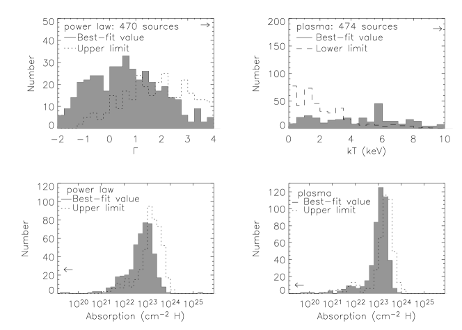
Figure 2: The distribution of the photon indices $\Gamma$, plasma temperatures $kT$, and absorption columns $N_{\rm H}$ derived from spectral fits to sources with at least 80 net counts. We have only included those sources that are consistent with the spectral models at the 95% confidence level. The filled histogram represents the best-fit values. The upper limits from the 90% uncertainty (single parameter of interest) on $\Gamma$ and $N_{\rm H}$ are indicated with the dotted histograms, and the lower limit on $kT$ with the dashed histogram. The arrows indicate the numbers of sources with best-fit values outside the ranges of the plots. Most of the sources have hard spectra: the median photon index is $\Gamma=0.7$, while we were only able to obtain lower limits on $kT$ from the plasma modes. The median absorption column is $6\times 10^{22}$ cm^-2.

in which we removed the assumption that the dust was optically thin. The column depth of dust was set to $\tau=0.485\cdot N_{\rm H}/(10^{22}{\rm cm}^{-2})$, and the halo size to 100 times the PSF size (Baganoff et al., 2003). In Table 2 we list the parameters of the best-fit spectral models: the column densities $N_{\rm H}$, either the power-law slope $\Gamma$ or the temperature $kT$, the observed and de-absorbed 2–8 keV fluxes, and the reduced $\chi^{2}$. The uncertainties are 90% confidence intervals ($\Delta\chi^{2}=2.71$). We also indicate sources from which the spectra should be viewed with caution, of which there are three categories: confused sources for which the radii of their PSF overlap those of a nearby source by more than 25%, sources that were near chip edges, and sources with variability (Section 2.4). About 25% of the sources are flagged in this manner.

We consider a spectrum to be adequately reproduced by a model if the chance probability of obtaining the derived value of $\chi^{2}$ is greater than 5%. Of the 566 sources that we modeled in this manner, the spectra of 470 could be modeled with an absorbed power law, and 469 could be modeled with an absorbed, collisionally-ionized plasma. Both spectral models were consistent with the data for 440 sources, because of limited statistics and the small bandpass over which photons are detected (for most sources, Galactic absorption prevents photons $<2$ keV from reaching the detector, while the effective area of the ACIS-I is small above 8 keV). Only 30 sources could be modeled with a power law but not a thermal plasma, while 29 sources could be modeled by a thermal plasma but not a power law. Finally, 67 spectra deviated from both continuum models at the 95% level. About 25 of these resemble statistical fluctuations, 30 are bright sources that appear to require multiple continuum components, and 12 exhibited strong iron emission between 6 and 7 keV.

For individual sources, the uncertainties on the spectral parameters are rather large. However, it is possible to draw some general conclusions about the population of X-ray sources from Table 2. In Figure 2, we plot the distributions of the best-fit absorption columns and photon indices or temperatures for all of those sources that Figure 3: Plot of the best-fit power-law spectral index ($\Gamma$) as a function of the observed 2–8 keV flux. Representative uncertainties on $\Gamma$ are indicated for a few points. There is no correlation between $\Gamma$ and the flux.

were adequately fit with the simple absorbed continuum model. As was mentioned in Muno et al. (2003a), 265 out of 470 of the point sources have power-law spectra with $\Gamma<1$, even after accounting for the absorption column. However, only 77 sources have 90% confidence limits for which $\Gamma<1$, and some of the apparent hardness of their spectra is due to line emission from Fe between 6–7 keV (see Section 2.2). Not surprisingly, the hard sources also have high best-fit temperatures under the thermal plasma model. However, because of the poor statistics and small bandpass, the temperatures are unconstrained in one-third of the sources, and there are only 21 sources with 90% lower limits on the temperatures that are $>10$ keV. The slopes of the spectra are not correlated with the intensities of the sources (Figure 2.1).

The median absorption column toward the the sources is $6\times 10^{22}$ cm^-2 for a power-law continuum, and $11\times 10^{22}$ cm^-2 for a thermal plasma continuum. The median value for the power-law continuum is identical to the column that is inferred from the $K$-band extinction toward Sgr A^∗ (see Tan & Draine, 2003, for a summary), while that for a thermal plasma continuum is twice as high. The difference between the median values results from the facts that (1) for a faint, hard source the values of $N_{\rm H}$ and the spectral slope cannot be determined independently, and (2) the thermal plasma continuum, can appear no harder than a $\Gamma\approx 1.5$ power law. Therefore, the thermal plasma models produce a higher median value of $N_{\rm H}$. Under either model, 30% of the sources are inferred to have a absorption column of $>10^{23}$ cm^-2. The one source that appears to be absorbed by more than $10^{24}$ cm^-2, CXOGC J174539.3–290027, is relatively faint, and the spectrum is poorly constrained.

Finally, we note that these spectra have been modeled assuming that all of the X-rays from a given source are absorbed by a single column of material. If we assume instead that a fraction of the X-ray emitting region is absorbed by a higher column (so-called “partial covering” models) an acceptable fit can be obtained for an arbitrary range of continuum shapes, because the bandpass over which we measure the spectrum is limited.

Figure 4: Comparisons of the chance probability that an iron line would be detected from sources, derived using Markov-Chain Monte Carlo simulations and using the $F$-distribution. The $F$-distribution generally over-estimates the chance probability of the line, which would cause the significance of a line to be under-estimated.

2.2 Iron Emission

Visual inspection of the 67 sources for which the simple continuum failed to reproduce their spectra indicates that $\approx 20$% exhibit residuals between 6–7 keV that may represent line emission from Fe. Therefore, we have performed a uniform search for Fe line emission from the brightest sources with hard spectra. We selected only those sources with more than 160 net counts, because we found that fainter sources were unlikely to provide more than one spectral bin between 6–7 keV. Likewise, we selected only those sources that were best-fit by absorbed power laws with $\Gamma<5$, because sources with steeper spectra were typically background-dominated above 6 keV. There were 183 sources that met both of these criteria. We modeled each source with an absorbed power law plus a Gaussian line that was fixed at either 6.4 keV to search for low-ionization (“neutral”) Fe emission, or at 6.7 keV to search for He-like Fe. The widths of the lines were fixed at 100 eV, to account for the fact that both the low-ionization and He-like lines are actually a blend of multiple transitions (e.g., Nagase et al., 1994).

To evaluate the significance of the added line, we computed a statistic $f$ from the reduction in $\chi^{2}$ provided by the more complex model:

$$f={{(\chi^{2}_{s}-\chi^{2}_{c})}\over{(\nu_{s}-\nu_{c})}}{{\nu_{s}}\over{\chi^{2}_{s}}},$$ (1)

where $\chi^{2}_{c}$ and $\chi^{2}_{s}$ are the values with and without the line, and $\nu_{c}$ and $\nu_{s}$ are the numbers of degrees of freedom for the fits ($\nu_{s}-\nu_{c}=1$, here). Unfortunately, because the null result of our more complex model, a line of zero flux, lies on a boundary of the parameter space we are considering (i.e., an emission line with negative flux is not physical, so the hard lower limit to the line flux is 0), $f$ is not distributed according to the $F-$distribution (Protassov et al., 2002). Therefore, we have simulated the expected distribution of $f$ for each of our sources using the Markov-Chain Monte Carlo technique described in Arabadjis et al. (2003). This technique allows us to evaluate the chance probability of observing a value of $f$ given (1) the statistical distributions of $N_{\rm H}$, $\Gamma$, and

Figure 5: The strength of line emission at left panels: 6.4 keV from low-ionization Fe, and right panels: 6.7 keV from He-like Fe. The top panels display histograms of the equivalent widths of the iron lines. The rightward-pointing arrow denotes the the four sources that may have iron emission with equivalent width $>2500$ keV. Most of these sources have very steep ($\Gamma>4.5$) spectra, and so the excess emission between 6–7 keV could represent either a hard continuum component, or poor background subtraction. However, the line from one of the sources with 6.4 keV iron emission with equivalent width $>2500$ eV appears to be real (CXOGC J174617.2–285449). The bottom panels illustrate how the measured equivalent widths are correlated with the photon flux from a source. Iron emission can only be detected in the fainter sources if it has a high equivalent width.

Figure 6: Combined spectrum of all Galactic center point sources with fewer than 500 net counts, before background subtraction. The background spectrum is taken to be that of the diffuse emission, and is indicated with the dashed curve.

the normalization from the fit, (2) the method used to group the spectral bins, and (3) the spectrum assumed for the background subtraction. Between 100–1000 simulations were computed for each source. We present in Figure 2.1 a comparison of the chance probabilities derived from the theoretical $F$-distribution and from the Monte Carlo simulations. In general, the theoretical $F$-distribution significantly under-estimates the significance of a line (the chance probability is deemed to be too large), although in 10% of the cases the theoretical distribution over-estimates the significance. This demonstrates the necessity of performing simulations in order to estimate the significance of an added line feature.

We have listed those sources with significant line emission in Table 3. We consider a line to be detected if it has less than a 1% chance probability of arising from random variations in the continuum, and if the fit produced $\chi^{2}_{c}/\nu_{c}<2$. In total, 35% (64 out of 181) of the sources that we examined have significant Fe line emission. We find that 25% of sources exhibit a significant line near 6.7 keV, while 16% of sources exhibit emission at 6.4 keV. There are 15 sources with significant lines at both 6.4 and 6.7 keV, but these tend to be faint sources in which it is not possible to constrain the line energy. We plot histograms of the equivalent widths and the equivalent widths as a function of the flux in Figure 5. For both species, the equivalent widths range from 200 eV to 5 keV. The median equivalent widths were 370 eV for the 6.4 keV Fe line, and 530 eV for the 6.7 keV Fe line. Six sources have lines with equivalent widths greater than 1 keV that appear upon visual inspection to be real. There are two systems with apparent equivalent widths $>10$ keV, but these have steep continuum spectra with $\Gamma>4.5$, and the excess emission between 6–7 keV represents either a hard continuum component or poor background subtraction. When line emission is not detected, the median 1-$\sigma$ upper limits to the line equivalent widths are 220 eV for He-like Fe, and 240 eV for low-ionization Fe.

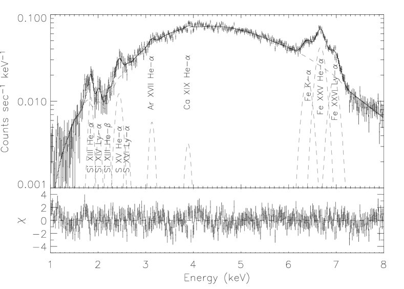
Figure 7: Combined, background-subtracted spectrum of the Galactic center point sources with fewer than 500 net counts. The best-fit model of a power-law plus 10 Gaussian lines is over-plotted. The expected centroid energies of lines from Si, S, Ar, Ca, and Fe are indicated.

2.3 Combined Spectra of Point Sources

In order to understand the average spectra of the Galactic center point sources, we summed the spectra of sub-groups of the individual point sources. We selected only those sources that were not detected below 1.5 keV with wavdetect, as these are most likely to lie near the Galactic center. We also excluded sources brighter than 500 net counts, because these sources provided individual spectra of good quality. We computed average effective area and response functions by averaging those from the individual sources, weighted by the number of counts from each source. We estimated the average background by extracting a spectrum from the rectangular region that traced the orientation of the ACIS-I detector during the 500 ks series of observations from 2002 May to June. We excluded from the background spectrum events that fell within circles circumscribing the 95% contour of the PSF around any point sources.

In Figure 2.2, we display the summed spectra of the Galactic center point sources with fewer than 500 net counts. The spectrum below 2 keV is dominated by the diffuse emission from the Galactic center. In Figure 2.2 we display the background-subtracted spectrum. The instrumental Ni line at 7.5 keV is absent from the spectrum, which indicates that the background subtraction was successful. Lines of Si, S, and Ar are also weak or absent in the spectrum of the point sources, in contrast to that of the diffuse emission (dashed line in Figure 2.2). Prominent lines from He-like and H-line Fe are evident at 6.7 and 6.9 keV, while weak, fluorescent K-$\alpha$ emission from low-ionization Fe is evident at 6.4 keV.

We modeled this spectrum using two approaches. First, we modeled the emission phenomenologically, using a power-law continuum and Gaussian line emission from Si, Figure 8: Ratio of the spectra of point sources with between 80 and 500 net counts to those with $<80$ net counts. The ratio is flat between 2.5–6 keV, which indicates that the continuum shapes are nearly identical. The deviations at 2.4 keV are due to stronger S emission in the brighter sources. The deviations between 6–7 keV are due to the range of strengths in the neutral, He-like, and H-like lines of Fe.

S, Ar, Ca, and Fe. The lines we included were chosen by examining whether lines from the strongest transitions from Table 1 in Mewe, Gronenschild, & van den Oord (1985) significantly improved the residuals when comparing the model to the data. For the final model, we placed lines at the energies expected for the He-like $n=2-1$ transitions of Si, S, Ar, Ca, and Fe; the He-like $n=3-1$ transitions of Si and S; the H-like $n=2-1$ transitions of Si, S, Ar, and Fe; and low-ionization Fe K-$\alpha$ at 6.4 keV. This model allowed us to measure and compare the equivalent widths of the lines. We also used a model consisting of two thermal plasma components, each of which was absorbed by a separate column of gas. This model is identical to the model used for the diffuse emission by Muno et al. (2004). We also note that this model is qualitatively similar to the multi-temperature, multi-absorber models typically used to model the accretion shocks in magnetized CVs (e.g. Ramsay et al., 2004a).

Several assumptions were required for the models to reproduce the data. First, we only applied the model between $1.0-8.0$ keV. Below this energy range the photon counts are dominated by foreground diffuse emission, while above this range the ACIS-I has a small effective area. Second, when modeling individual lines with Gaussians, the widths of the lines from He-like Si, S, and Fe and low-ionization Fe were allowed to be as large as $\approx 70$ eV to account for the fact that the lines are blends of several transitions that cannot be resolved with ACIS. Third, we allowed for a $\lesssim 1$% shift in the energy scale in each spectrum because of uncertainties in gain calibration of our CTI-corrected data. When fitting Gaussians to the He-like transitions and the 6.4 keV line of Fe, the line centroids were varied one-by-one until they achieved best-fit values, and then frozen. When using plasma models, the red-shift parameter was used to change the energy scale in a similar manner. Finally, a 3% systematic uncertainty was added in quadrature to the statistical uncertainty in order to account for uncertainties in the ACIS effective area.

To account for absorption in each model we assumed (1) Figure 9: Combined spectrum of Galactic center point sources with fewer than 500 net counts and sorted according to their hard color. Although the observed shape of the continuum varies strongly with hardness ratio, lines from He-like and H-like Fe are present in all three groups of sources. The ratios of the Fe lines are consistent with a $kT\approx 8$ keV plasma in all cases. This suggests that variations in the local absorption column toward the sources cause the variations in the apparent hardness of the Galactic center sources.

that the entire region was affected by one column of material that represents the average Galactic absorption (modeled with phabs in XSPEC) and (2) that a fraction of each region was affected by a second column that represents absorbing material that only partially-covers the X-ray emitting region (modeled with pcfabs). This partial-covering absorption model produces a low-energy cut-off that is less steep than that which would be produced by a single absorber. The model can roughly account for the fact that both the point sources and absorbing material are distributed along the line of sight. The mathematical form of the model was

$$e^{-\sigma(E)N_{\rm H}}([1-f_{\rm pc}]+f_{\rm pc}e^{-\sigma(E)N_{\rm pc,H}}),$$ (2)

where $\sigma(E)$ is the energy-dependent absorption cross-section, $N_{\rm H}$ is the absorption column, $N_{\rm pc,H}$ is the partial-covering column, and $f_{\rm pc}$ is the partial-covering fraction. Dust scattering was not included, because when modeling the spectrum its optical depth was degenerate with the partial-covering fraction $f_{\rm pc}$.

2.3.1 Phenomenological Model

Since the natures of these point sources are uncertain, the most straightforward way of modeling their spectrum is with an absorbed power-law continuum and Gaussian line emission. The average spectrum of sources with fewer than 500 net counts is displayed along with the model spectrum in Figure 2.2. The model parameters are listed in the first column of Table 4. After some initial tests, we found that $f_{\rm pc}$ was poorly constrained, but the best-fit values were near 0.95. We therefore fixed $f_{\rm pc}$ to this value. The remaining parameters were allowed to vary. The total absorption column, $N_{\rm H}+N_{\rm pc,H}\approx 9\times 10^{22}$ cm^-2, is slightly higher than the expected Galactic value. Simulations in XSPEC indicate that this is probably because we did not include dust scattering, which produces about 30% of the total absorption. The inferred continuum is flat, with photon index $\Gamma=0.8$, which is similar to the median value from the individual sources, $\Gamma=0.7$. Finally, the equivalent width of the He-like Fe line is 400 eV, which is similar to that observed from individual bright sources. The strength of the neutral Fe line is considerably lower than those detected from the individual sources, although this is not surprising since fewer of the individual sources exhibit 6.4 keV lines than do 6.7 keV lines (see Section 2.2).

We then examined how the average spectra of the point sources varied with flux. We compared the summed spectra of sources with fewer than 80 net counts to those with 80–500 net counts, because these two groups of sources produce nearly the same numbers of net counts ($\approx 7.5\times 10^{5}$). The best-fit parameters of our phenomenological model of these spectra are listed in the second two columns of Table 4. Both the absorption column and photon index were slightly larger in the bright sources. However, the continuum shape looks very similar by eye. To highlight this, in Figure 2.3 we plot the ratio of the averaged spectra of sources with 80–500 net counts to that of sources with $<80$ net counts. The only differences in the continuum spectra are above 7 keV, which may indicate that the faint sources produce slightly more high-energy flux. Differences in the equivalent widths of the line emission are also evident in Figure 2.3. The equivalent width of the Fe XXV He-$\alpha$ emission was 30% higher in the fainter sources (3.7$\sigma$), and the equivalent width of neutral Fe K-$\alpha$ was a factor of 2 lower in the faint sources (4.9$\sigma$). There is also a factor of 3 less S He-$\alpha$ emission in the faint sources (4.3$\sigma$). We also split the data into smaller flux intervals, and found similar results. Thus, the continuum spectra of the point sources change very little with intensity, but the S and Fe lines range over a factor of $\gtrsim 2$ in equivalent width.

We also examined the combined spectra as a function of the hard color, which provides a measure of the steepness of the spectrum. The hard color is defined as $HR=(h-s)/(h+s)$, where $h$ is the number of counts in a hard band from 4.7–8.0 keV, and $s$ is the number of counts in a softer band from 3.3–4.7 keV. We divided the data using three ranges in hard color, guided by the expected power-law index from simulations with PIMMS (Muno et al., 2003a): $HR>0.2$ for sources with $\Gamma\approx 0$ spectra, $-0.1<HR<0.2$ for sources with $\Gamma\approx 1.5$ spectra, and $HR<-0.1$ for sources with $\Gamma>2$ spectra. The spectra are plotted in Figure 2.3, and the best-fit parameters for the phenomenological model are listed in the last three columns of Table 4. We find that the sources with larger $HR$ have continuum spectra that are intrinsically flatter, at least given our model for the interstellar and intrinsic absorption. We also find significant changes in the line strengths, although there is no monotonic trend with $HR$.

2.3.2 Two-$kT$ Plasma Model

We next modeled the spectra of the point sources as originating from two thermal plasmas, each of which was absorbed by a separate component as parameterized in Equation 2, as well as emission from low-ionization Fe at 6.4 keV. The parameters of the best fit models to the average spectra for the groups of sources used in the previous section are all listed in Table 5. The values of $\chi^{2}_{\nu}$ are generally larger under the plasma models than under the phenomenological models, because the plasma models predict too little flux above 7 keV. However, the plasma models do provide a good qualitative description of the data. The weak lines from Si, S, and Ar require cool plasmas with $kT_{1}\approx 0.5$ keV; this component appears to be visible only in sources with $HR<-0.1$. The abundances of Si and S appear to be significantly below solar values in the soft sources, where the lines are most clearly detected. The He-like and H-like Fe lines require hotter plasmas with $kT_{2}\approx 8$ keV. The abundances of Fe are also generally about 50% solar, although they are consistent with the solar ones in the faintest and softest sources.

The temperatures of these plasma components are very similar to those inferred from the diffuse emission, because emission lines from the same set of ions are present in both spectra (Muno et al., 2004). However, in contrast to the diffuse emission, the cooler plasma in the point sources is heavily absorbed and contributes little to the observed flux.

More importantly, the presence of prominent He-like and H-like Fe emission from $kT=7-9$ keV plasma in all groups of sources suggests that the X-ray emission is produced by similar physical mechanisms.

2.4 Search for Variability

We searched for variability in the 0.5–8.0 keV bandpass from the entire sample of X-ray sources from Muno et al. (2003a), in order to identify flux changes that occurred within single observations, and long-term variations in the mean flux between observations.

2.4.1 Short-term Variability

Figure 10: Example light curves of variable sources in the field. To compute the resulting photon fluxes, the total counts received from each source as a function of time have been divided by the mean value of the detector effective area from each observation.

To search for short-term variability, we applied a Kolmogorov-Smirnov (KS) test to the un-binned arrival times of the events during each observation. Before performing the search, we removed events flagged as potential cosmic ray after-glows. We also excluded data received near the edges of the detector chips, and data from the first part of ObsID 1561 for sources that were within 5.5′ of the bright transient GRS 1741.9$-$2853 (Muno et al., 2003b). If the cumulative distribution of the arrival times differed

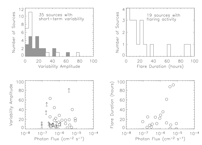
Figure 11: Summary of the amplitudes and durations of the variability in sources detected toward the Galactic center. The top left panel displays a histogram of the ratio of the maximum to the minimum flux from each variable source. Sources that were detectable at minimum are indicated with solid histogram, while lower limits on the variability amplitude are illustrated with the open histogram. The bottom left displays the variability amplitude (or lower limits thereto) as a function of the mean photon flux from the source. Not surprisingly, small-amplitude variability can only be detected if a source is bright. The top right panel displays a histogram of the durations of flare-like events. These range from $<1$ ks to nearly 100 ks. The bottom right panel illustrates that the observed flare duration is not strongly correlated with the mean photon flux from a source.

from a uniform distribution (which would imply a constant flux) with greater than 99.9% confidence in any observation, we considered the source to vary on short time-scales. We find that 18 foreground sources and 21 Galactic center sources are variable on short time scales according to the KS test. We list these sources in Table 6. Examples of short-term variability are shown in the bottom three panels of Figure 10.

To characterize the duration and amplitude of the variability, we have applied the“Bayesian Blocks” algorithm of Scargle (1998) (see also Eckart et al., 2004). The algorithm is based on a parametric maximum-likelihood model of a Poisson process that divides the data into sequential segments, each of which has a constant count rate. The segments were identified by dividing the events into sub-intervals, and computing the odds ratio that the count rate has varied. If variability was found, then each interval was split further into sub-intervals, in order to track the structure of the variability. We found that by using an odds ratio corresponding to a 67% chance that the variation is real, we could identify changes in the flux from all but four of the variable sources. If the Bayesian Blocks code identified only two intervals with differing count rates, then the variability was classified as a “step” function. If it identified more than two intervals with differing count rates, we defined the variability as a flare; a search of the data revealed no instances of dips, which are unlikely to be detected in sources with low count rates. We computed the background-subtracted maximum and minimum count rates for each variable observation, and divided them by the mean value of the effective area function for that source to convert them into photon fluxes. The maximum and minimum fluxes are listed in Table 6. We also list the durations of the flares in kiloseconds, and either the ratio between the maximum and minimum flux, or the lower limit thereto if the baseline flux is an upper limit. The photon fluxes in the table can be converted to energy fluxes by the factors 1 ph cm^-2 s^-1$=3\times 10^{-9}$ erg cm^-2 s^-1 (0.5–8.0 keV) for foreground sources, and 1 ph cm^-2 s^-1$=8\times 10^{-9}$ erg cm^-2 s^-1 (2–8 keV) for Galactic center sources. The peak luminosities of the variable Galactic center sources typically range from $6\times 10^{31}$ to $1.7\times 10^{33}$ erg s^-1. However, one flare from CXOGC J174552.2–290744 consists of 5 photons received in 100 s and has a peak luminosity of $10^{34}$ erg s^-1. None of the events in the apparent flare were flagged as cosmic rays by the CXC pipeline, and tests of Figure 12: Summary of the amplitudes and durations of the variability observed between observations in sources detected toward the Galactic center. The top panel displays a histogram of the ratio of the maximum to the minimum flux from each source with long-term variability. Sources that were detectable at minimum are indicated with solid histogram, while lower limits on the variability amplitude are illustrated with the open histogram. The bottom displays the variability amplitude (or lower limits thereto) as a function of the mean photon flux from the source. Once again, small-amplitude variability can only be detected if a source is bright.

events from elsewhere on the detector that were flagged as cosmic rays indicate that they deposit their energy on time scales of $\lesssim 20$ s, so we consider the flare real. No source exhibits flares similar to those seen about once a day from Sgr A^∗, with durations of $\approx 1$ h and $L_{\rm X}\gtrsim 10^{34}$ erg s^-1.

Figure 11 displays histograms of the variability amplitude and the durations of the flares. Nearly half of the variability has a peak flux over 10 times the quiescent level. In the bottom-left panel, we plot the amplitude of the variability as a function of the mean flux from each source. The amplitudes of the variability are not a strong function of the mean flux from the source. However, we are unable to detect the faintest sources when they are in their low-flux states, so for these sources we only can report lower limits to the variability amplitude. The flare durations are spread fairly evenly, with a median duration of about 20 ks. As can be seen from the bottom-right panel of Figure 11, the flare durations show no correlation with the mean flux from a source.

In order to quantify our sensitivity to short-term variations, we need to examine the probability that a change in count rate could be detected. If we assume a baseline count rate $r_{l}$ persists for a time $t_{l}$, and that a flare occurs with count rate $r_{h}$ lasting $t_{h}$, then the total number of counts in each interval follows the Poisson distribution. Therefore, the joint probability that the measured baseline count rate $N_{l}/t_{l}$ is less than the measured flare count rate $N_{h}/t_{h}$ is

$$P(N_{h}>N_{l}t_{h}/t_{l})=$$

$$\sum_{N_{l}=0}^{\infty}\left({{(r_{l}t_{l})^{N_{l}}e^{-r_{l}t_{l}}}\over{N_{l}!}}\sum_{N_{h}>N_{l}t_{h}/t_{l}}^{\infty}{{(r_{h}t_{h})^{N_{h}}e^{-r_{h}t_{h}}}\over{N_{h}!}}\right).$$ (3)

This probability represents the chance that a flare of amplitude $r_{h}/r_{l}$ would be detected.

The median net counts from the sources in the catalog of Muno et al. (2003a) was 49, with a background of 52 counts. These values translate to count rates of $n=7.8\times 10^{-5}$ count s^-1 net and $b=8.3\times 10^{-5}$ count s^-1 background. If we use $r_{l}=n+b$ in Equation 3, a 36 ks flare during the long 150 ks observation could be detected with an amplitude a factor of $\approx 10$. Such a flare could be detected from half of the sources in our sample. On the other hand, a flare that reaches twice the quiescent flux level for 36 ks could only be detected if the quiescent count rate was $r_{l}=2\times 10^{-3}$ count s^-1. Only 17 sources are this bright, so such a small-amplitude flare would generally be unobservable. Not surprisingly, all of the short-time scale variability with amplitudes $<3$ are long duration, step-like changes in flux.

2.4.2 Long-term Variability

To search for long-term variability, we computed the value of $\chi^{2}$ for the photon fluxes in each observation under the assumption that the mean rate was constant. We computed the approximate total (source plus background) photon flux by dividing the total number of counts detected by the live time and the mean value of the effective area function. To compute a net flux, we then subtracted a background count rate, which was estimated in the same manner as for the spectrum. We considered a source as variable if the photon fluxes both before and after background subtraction were inconsistent with a constant mean value with more than 99% confidence. We excluded sources with short-term variability when searching for long-term variability. We also excluded data from the first part of ObsID 1561 for sources that were within 5.5′ of the bright transient GRS 1741.9$-$2853. Long-term variability is illustrated in the top three panels of Figure 10.

We find that 20 foreground sources and 77 Galactic center sources vary on long time scales. We list in Table 7 the minimum and maximum background-subtracted photon fluxes for the variable sources. We present a histogram of the ratio of the maximum to minimum fluxes in the top panel of Figure 2.4.1. Most of the ratios are upper limits, because the sources are not detected at their minimum flux levels. The bottom panel illustrates the variability amplitudes as a function of the mean intensity of each source. There is no apparent correlation between the amplitude and intensity of the source.

We can quantify our sensitivity to long-term variations in the same manner as for short-term variability, using Equation 3. The most extreme form of long-term variability is that of a source that is bright for some portion of the observations lasting a total time $t_{h}$, and decreases below the background level for the remaining observations lasting a time $t_{l}$. We therefore assume that the total counts from a source is consistent with the background $b=8.3\times 10^{-5}$ count s^-1 during the time $t_{l}$ when it is faint. If the source is “off” during one of the 12 ks observations, we could detect this decrease in count rate with 99% confidence if during the remaining 614 ks of observations the source was brighter than $3\times 10^{-4}$ net count $s^{-1}$. Approximately 9% of the sources are this bright. We could detect variability from a source that is “off” during all but the 500 ks monitoring campaign (2002 May–June) if the count rate at maximum was $8\times 10^{-5}$ count s^-1, which is valid for half of the sources searched.

3 Discussion

The large number of sources detected toward the Galactic center is most likely a product of the large density of stars there. The 17′ by 17′ field spans a physical distance of 20 pc in projection from Sgr A^∗, and therefore probes the inner regions of the Nuclear Bulge that was studied extensively by Launhardt, Zylka, & Mezger (2002). Using their models, we estimate that $1.3\times 10^{8}$ $M_{\odot}$ of stars lie within a cylinder of radius 20 pc and depth 440 pc that is centered on the Galactic center. Thus, our observation encompasses up to 0.1% of the total Galactic stellar mass, which is $\sim 10^{11}$ $M_{\odot}$. However, we have also found that the surface density of the X-ray sources falls off as $\theta^{-1}$ away from Sgr A^∗, so it is possible that most of the X-ray sources lie in an isothermal sphere of radius 20 pc (Muno et al., 2003a). Such a sphere would contain $3\times 10^{7}$ $M_{\odot}$ of stars, or 0.03% of the

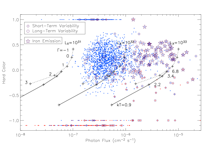
Figure 13: Summary of the spectral and variability properties of the X-ray sources detected toward the Galactic center. For all of the sources in the sample, we plot the hard color against the photon flux. The hard color is defined as $HR=(h-s)/(h+s)$, where $h$ is the number of counts in a hard band from 4.7–8.0 keV, and $s$ is the number of counts in a softer band from 3.3–4.7 keV. We were able to derive hard colors for 1848 out of 2357 sources. Sources that are only detected in the 4.7–8.0 keV band are given values of 1. Sources that are only detected in the 3.3–4.7 keV band are given values of $-1$. Sources detected in neither band are given hard colors of $-1.1$. Sources located at or beyond the Galactic center are indicated in blue, while foreground sources are indicated in red. We use solid lines to illustrate the hard colors and photon fluxes expected for thermal plasma with a range of temperatures and luminosities (bolometric for $d=8$ kpc), and the dotted lines for power laws with a range of photon indices and luminosities (0.5–8 keV). We also indicate which sources exhibit iron lines (stars) and short-term variability (diamonds) or long-term variability (circles). Note that sources with short-term variability were not searched for long-term variability.

Galactic stellar mass. For comparison, the shallower survey carried out by Wang et al. (2002) covered the entire Nuclear Bulge (albeit with a factor of 5 less sensitivity), and thus sampled $\sim 1$% of the mass of stars in the Galaxy. The stellar density at the location of the X-ray sources is between 240–900 $M_{\odot}$pc^-3 (for a 20 by 440 pc cylinder and a 20 pc sphere, respectively), compared to 0.1 $M_{\odot}$ pc^-3 in the local stellar neighborhood (Binney & Tremaine, 1994, p. 16). We will keep these numbers in mind as we consider the likely natures of the Galactic center point sources.

The sample identified as part of the Chandra observations of the Sgr A^∗ field is unique, because the long exposure time allows us to detect faint sources ($F_{\rm X}=(3-100)\times 10^{-15}$ erg cm^-2 s^-1, 2–8 keV), whereas the strong diffuse X-ray emission and the high absorption toward the Galactic center prevent us from observing X-ray sources unless they are prominent in the 4–8 keV band. Prior to Chandra, the most sensitive hard X-ray survey of the Galactic plane was taken with ASCA. That survey identified only 163 sources, with a detection limit of $\approx 3\times 10^{-13}$ erg cm^-2 s^-1 (2–10 keV; Sugizaki et al., 2001). The Galactic center sources are on average much harder than those detected in the ASCA survey. The brighter ASCA sources had a median photon index of $\Gamma=2.5$, with only 15% of the sources having $\Gamma<1$, while the fainter Chandra sources have a median $\Gamma=0.7$ (Figure 2). The difference in hardness of the two samples is probably a selection effect caused by the high absorption and the strong diffuse emission toward the Galactic center. The X-ray sources that we have studied in this paper probably sample only the hardest examples of the population identified with ASCA.

Likewise, Chandra observations of globular clusters have identified a couple hundred X-ray sources with $L_{\rm X}=10^{29}-10^{33}$ erg s^-1(Grindlay et al., 2001; Pooley et al., 2002; Becker et al., 2003; Heinke et al., 2003a, b). These luminosities overlap those inferred for the sources near the Galactic center in our sample. However, only a few of the $\approx 60$ globular cluster sources with spectral information are best modeled by a $\Gamma<1$ power-law. Most have steeper spectra that are consistent with $\Gamma>1.5$ power-laws or $kT\approx 1-20$ keV thermal plasmas.

In addition to the hardness of their spectra, the X-ray sources detected toward the Galactic center share several other interesting properties. Most notable is line emission from low-ionization, He-like, and H-like Fe (Figures 5 and 2.2). On average, the low-ionization Fe lines have equivalent widths of 100–230 eV, while the He-like Fe lines have equivalent widths of 350–450 eV. The strengths of these lines range over a factor of two when considering sources with a range of intensity and spectral hardness (Table 4). However, in all cases the average ratios of the He-like and H-like lines are consistent with those expected from a thermal plasma of $kT\approx 8$ keV (Table 5). The presence of these Fe lines in a large fraction of the sources suggests that they could be dominated by a single population of sources.

However, the emission from such a plasma should produce a much steeper continuum spectrum, with $\Gamma\approx 1.5$ instead of $\Gamma\approx 0.7$. Unfortunately, it is not possible to determine unambiguously the physical process producing the X-ray emission from the continuum and iron lines alone. For instance, if the X-ray emitting regions are partially absorbed by material local to the X-ray sources, the observed spectra can be much harder than the intrinsic ones. Alternatively, the line emission could be produced in photo-ionized plasmas, although the large equivalent widths of the lines indicates that the continuum emission exciting them must not be observed directly (e.g. Mukai et al., 2003). In either of these cases, the intrinsic X-ray luminosity would be significantly higher than is inferred from the flux received with Chandra.

While the average spectral properties provide an overview of the characteristics of the X-ray sources near the Galactic center, it is still important to examine the properties of individual sources to determine how various classes of sources contribute to the population there. Therefore, in Figure 13 we display the spectra and intensities of individual sources by plotting the hard color of each source against its photon flux. These quantities are measures of the physical quantities of interest, the intrinsic spectral shape and the luminosity of a system. We also indicate in Figure 13 the expected hardness ratios and photon fluxes for sources over a range of luminosities and with either (1) thermal plasmas over a range of temperatures $kT$ (solid lines), or power laws over a range of photon indices $\Gamma$ (dotted lines). In all cases, we have assumed the sources are absorbed by the median column density from the spectral models, $6\times 10^{22}$ cm^-2 of gas and dust. Approximately 75% of the 2000 Galactic center X-ray sources are detected with 90% confidence in both the 3.3–4.7 and 4.7–8.0 keV bands, and therefore have hard colors in Figure 13.

We also indicate in Figure 13 which sources exhibit line emission from Fe. Nearly all of the sources brighter than $4\times 10^{-6}$ ph cm^-2 s^-1 and harder than $HR=0$ exhibit line emission from He-like Fe. This is not surprising, given the prominence of line emission in the average spectra. Fe emission is detected less often in fainter sources, but this is probably due to lower signal-to-noise.

Finally, we indicate which sources exhibit variability. The sources that are identified as variable tend to be brighter, because the signal-to-noise is better. Soft sources are most likely to exhibit short-term variability.

In the following sections, we use these properties to guide our discussion of the natures of the sources. The luminosities of the Galactic center sources are consistent with those of young stellar objects (YSOs), interacting binaries (RS CVns), Wolf-Rayet (WR) and early O stars, cataclysmic variables, quiescent black hole and neutron star X-ray binaries, and possibly the ejecta of recent supernova that are interacting with molecular clouds. We consider each in turn.

3.1 Sources with Active Stellar Coronae

Many stars produce X-rays in their magnetic coronae. In particular, K and M dwarfs are so numerous that they contribute significantly to heating the ISM (e.g., Schlickeiser, 2002). However, individually their X-ray emission is faint, with $L_{\rm X}<10^{29}$ erg s^-1, and cool, with $kT<1$ keV (e.g., Krishnamurthi et al., 2001). Although, most of the foreground sources are probably low-mass main sequence stars (P. Zhao, in preparation), few of the Galactic center sources should be. YSOs and RS CVns are significantly brighter, with $L_{\rm X}\approx 10^{29}$ to $10^{32}$ erg s^-1(e.g., Feigelson et al., 2002; Dempsey et al., 1993a), and are therefore more likely to be seen at the Galactic center.

3.1.1 Young Stellar Objects

The number of YSOs at the Galactic center will depend upon whether low-mass stars have formed there recently. For instance, if star formation proceeds at the Galactic center in a similar manner as it has in the Orion nebula, then the two-dozen massive, emission-line stars in the central parsec of the Galaxy could conceivably be accompanied by tens of thousands of low-mass YSOs (e.g., Feigelson et al., 2002). However, the strong tidal forces, milliGauss magnetic fields, and turbulent molecular clouds near the Galactic center may prevent low-mass stars from forming there (Morris, 1993).

YSOs have luminosities between $10^{29}-10^{31.7}$ erg s^-1, and spectra that can be described by thermal plasma emission with $kT=1-10$ keV (e.g., Priebisch & Zinnecker, 2002; Kohno, Koyama, & Hamaguchi, 2002; Feigelson et al., 2002). Therefore, any YSOs that are located near the Galactic center should be found in the bottom left of Figure 13, with $HR<0$ and fluxes $<2\times 10^{-7}$ ph cm^-2 s^-1. However, the detection threshold for sources with $HR<0$ is approximately $10^{31.5}$ erg s^-1, and only $\sim 0.4$% of YSOs are brighter than this limit (Feigelson et al., 2002). YSOs also commonly exhibit flares lasting several hours, but fewer than 0.1% exhibit flares brighter than $10^{32}$ erg s^-1 (Grosso et al., 2004; Feigelson, 2004). In contrast, the faintest genuine flare from a Galactic center source has a peak luminosity of $5\times 10^{32}$ erg s^-1, whereas only three sources with short-term variability have peak luminosities below $10^{32}$ erg s^-1. Therefore, we believe that even the flaring sources are unlikely to be YSOs, and that any population of YSOs remain largely undetected at the Galactic center.

3.1.2 Interacting Binaries

RS CVn systems are among the most numerous hard X-ray sources with $L_{\rm X}>10^{29}$ erg s^-1, with a local space density of $\approx 5\times 10^{-5}$ pc^-3 (Favata et al., 1995). Using the models of Launhardt et al. (2002) to scale the local number density to the stellar density at the Galactic center (Section 3), we estimate that the total number of RS CVns within 20 pc of the Galactic center is $\approx 1.5\times 10^{4}$, while the number within a cylinder of 20 pc radius extending the length of the nuclear bulge (440 pc) is $7\times 10^{4}$.

However, RS CVns would be difficult to detect near the Galactic center. They typically have soft spectra, with $kT\approx 0.1-2$ keV, and luminosities of $L_{\rm X}=10^{29}-10^{32}$ erg s^-1(e.g., Dempsey et al., 1993b; Singh, Drake, & White, 1996). Therefore, RS CVns would have $HR<-0.3$ and photon flux $<3\times 10^{-7}$ ph cm^-2 s^-1 in Figure 13. This portion of the figure is sparsely populated. Moreover, we are only sensitive to sources with $kT\lesssim 2$ keV if they are more luminous than $5\times 10^{32}$ erg s^-1, whereas only $\sim 2\%$ of RS CVns are this luminous (Dempsey et al., 1993a). Finally, although RS CVns do exhibit flares lasting several hours with amplitudes of up to a factor of ten, they are seldom more luminous than $\approx 10^{32.5}$ erg s^-1 (e.g., Tsuru et al., 1989; Franciosini, Pallavicini, & Tagliaferri, 2001, 2003). Therefore, these flares would not be observable in our Galactic center data. The difficulty of detecting RS CVns and the lack of good candidate objects indicates we have probably identified only a tiny fraction of the RS CVns at the Galactic center.

3.2 Winds from Massive Stars

There is currently significant debate about the origin of the X-ray emission from WR and early O stars (e.g., Waldron & Cassinelli, 2001), but it is generally thought that the X-rays are produced through shocks in their winds (see, e.g., Chlebowski & Garmany, 1991). They have luminosities of up to $\approx 10^{33.5}$ erg s^-1 in isolation, and $\approx 10^{35}$ erg s^-1 when two such stars are in a colliding-wind binary. Their spectra can usually be modeled as thermal plasma with $kT=0.1-6$ keV (e.g., Pollock, 1987; Portegies-Zwart et al., 2002). These systems would lie in the portion of the color-intensity diagram with $HR<0$ in Figure 13.

The number of these systems present near the Galactic center is unknown, because it is determined by the uncertain star formation history (see, e.g., Morris, 1993). Figer (1995) and Cotera et al. (1999) have identified several massive, emission-line stars associated with HII regions near the Galactic center, but none of these has counterparts in our X-ray catalog. The wide-area search that Figer (1995) conducted failed to turn up additional candidates. Still, the unique conditions at the Galactic center make it important to understand the number of massive stars there, so we suggest that the relatively soft X-ray sources would serve as good targets for future searches for massive stars.

3.3 Millisecond Pulsars

Isolated millisecond pulsars typically produce X-ray emission from particles accelerated as they spin down, with $L_{\rm X}=10^{28}-10^{31}$ erg s^-1 (Possenti et al., 2002). At these luminosities, millisecond pulsars would be undetectable at the Galactic center. However, Cheng et al. (2004) have predicted that the wind from a millisecond pulsar could produce $L_{\rm X}=10^{31}-10^{33}$ erg s^-1 by interacting with dense regions of the ISM ($n\gtrsim 100$ cm^-3). They suggest that $\sim 100$ millisecond pulsars could be present in our field, although the number of detectable systems would depend upon the volume of dense gas at the Galactic center. Muno et al. (2004) have demonstrated that a large fraction of the inner 20 pc of the Galaxy is filled with hot ($T\sim 10^{8}$ K), low density ($n\approx 0.1$ cm^-3), X-ray emitting plasma, so only a small fraction of isolated millisecond pulsars may be detectable. Moreover, their spectra should be power laws with $\Gamma=1.5-2.5$, which corresponds to $-0.2<HR<0.0$ in Figure 13. This places millisecond pulsars on the same portion of the hardness-intensity diagram as CVs and RS CVns. As discussed in Cheng et al. (2004), identifying candidate systems among the point sources would be difficult, but millisecond pulsars could account for extended features seen in the field (Morris et al., 2003).

3.4 Accreting Sources

3.4.1 Low-Mass X-ray Binaries

Neutron stars and black holes accreting from low-mass companions that over-fill their Roche lobes are typically identified in outburst with $L_{\rm X}>10^{36}$ erg s^-1, although the majority of their time is spent in quiescence with $L_{\rm X}<10^{34}$ erg s^-1. LMXBs have been observed extensively in quiescence. The spectra of quiescent neutron star systems have been described with a $kT\approx 0.3$ keV black body producing $L_{\rm X}\sim 10^{32}$ erg s^-1, plus a $\Gamma\approx 1-2$ power-law tail that contributes $L_{\rm X}\sim 10^{31}$ erg s^-1 (Asai et al., 1998; Kong et al., 2002a). The black hole systems have $L_{\rm X}\lesssim 10^{31}$ erg s^-1 and exhibit $\Gamma\approx 1-2$ power-law spectra (Rutledge et al., 2001; Wijnands et al., 2002; Campana et al., 2002a). The thermal emission from a neutron star would be unobservable behind $6\times 10^{22}$ cm^-2 of absorption, so is of little relevance to the current observations. The power-law components of both the neutron star and black hole systems would produce $-0.1<HR<0.2$.

However, LMXBs are rare — theoretical models predict that $\sim 10^{4}$ should currently be in quiescence in the entire Galaxy, whereas only only $\sim 100$ LMXBs, or 1%, have been identified (compare Iben, Tutukov, & Fedoroval, 1997; Belczynski & Taam, 2004). Thus, if LMXBs form at the Galactic center in a similar manner as in the disk, our observation should encompass $\sim 20$ of them (Belczynski & Taam, 2004). Transient outbursts from three LMXBs already have been identified within 10′ of the Galactic center (Eyles et al., 1975; Pavlinsky, Grebenev, & Sunyaev, 1994; Maeda et al., 1996). If these truly represent $\sim 20$% of the total number there, then it would appear that LMXBs near the Galactic center are considerably more active than those in the Galactic disk. Alternatively, LMXBs could be concentrated near the Galactic center through dynamical settling (e.g., Morris, 1993; Portegies-Zwart, McMillan, & Gerhardet al., 2003). In order to better constrain the numbers of LMXBs within the nuclear bulge, it is important to continue to monitor this region in order to search for transient outbursts from additional systems.

Prior to the Roche-lobe overflow phase, accretion onto the compact objects should also proceed at low rates from the winds of the low-mass companions (Bleach, 2002; Willems & Kolb, 2003; Belczynski & Taam, 2004). These pre-LMXBs should have $L_{\rm X}=10^{28}-10^{32}$ erg s^-1, and would probably resemble Roche-lobe overflow systems in quiescence. Up to $10^{5}$ systems could be present in the Galaxy, and $\sim 20-100$ in our image of Sgr A^∗(Willems & Kolb, 2003; Belczynski & Taam, 2004).

3.4.2 High-Mass X-ray Binaries

Neutron stars and black holes accreting from the winds of massive companions should be about as common as LMXBs, because although the massive companions have much shorter lifetimes, accretion can occur when the separations between the binary components are much larger ($\sim 1$ AU compared to $\sim R_{\odot}$; see Pfahl, Podsiadlowski, & Rappaport 2002). They could be particularly abundant near the Galactic center, because it appears that 10% of Galactic star formation is currently occurring within the nuclear bulge (Launhardt et al., 2002). Our observations encompass $\sim 5$% of the nuclear bulge, so it would not be unreasonable to assume that, of the $\sim 10^{4}$ HMXBs in the Galaxy, $0.1\cdot 0.05\cdot 10^{4}\sim 50$ could be present in the field around Sgr A^∗ (see Pfahl et al., 2002).

In both outburst and quiescence, black hole HMXBs generally resemble LMXBs, because their X-ray emission is produced entirely in the accretion flow. Neutron star HMXBs, on the other hand, usually look much different from their LMXB counterparts, because the neutron stars in the young, high-mass systems tend to be more highly magnetized ($B\gtrsim 10^{12}$ Gauss). Neutron star HMXBs in outburst produce X-rays from shocks that form in the magnetically-channeled column of accreted material. At the location of the shocks, the accretion flow is optically-thick, so the resulting spectra are flat, and can be described with a $\Gamma<1$ power law between 2–8 keV (e.g. Campana et al., 2001). Therefore, neutron star HMXBs should have $HR>0.1$ in Figure 13. HMXBs also sometimes exhibit line emission at 6.4 keV from fluorescent neutral material in the companion’s wind, as well as weaker emission from He-like Fe at 6.7 keV that is produced by photo-ionized plasma in the wind. Although large equivalent widths have been reported from low-resolution measurements with gas proportional counters (e.g., Apparao et al., 1994), the few measurements of these lines with CCD resolution spectra indicate that they have equivalent widths $\lesssim 100$ eV (e.g., Nagase et al., 1994; Shrader et al., 1999).

Since the strong magnetic fields around the neutron stars in HMXBs channel the accreted material onto the star’s polar caps, the surest way to identify neutron star HMXBs is through periodic modulations in their X-ray emission. We have found that seven hard Galactic center sources in our field exhibit periodic variability (Muno et al., 2003c). However, the periods are all $>300$ s, which makes it impossible to rule out that they are accreting white dwarfs. On the other hand, modulations with shorter periods would be rendered undetectable by Doppler shifts from orbital motion, so the lengths of the periods observed are not necessarily a strong constraint on the entire population of sources at the Galactic center.

Other variability is also seen from HMXBs. Short-term (several ks) flares are seen infrequently and are ascribed to instabilities in the accretion flow (e.g., Augello et al., 2003; Moon, Eikenberry, & Wasserman, 2003). Long-term variations are more common and are often caused either by changes in the density of the wind at the location of compact objects that have eccentric orbits around the donor star, or by instabilities in the excretion disks around the Be stars that are the mass donors in half of the known HMXBs (e.g. Apparao et al., 1994).

The above considerations suggest that faint, neutron star HMXBs can account for some fraction of the hard Galactic center point sources. The main problem with this hypothesis is that few HMXBs have been observed at $L_{\rm X}<10^{34}$ erg s^-1, and the ones that have can be described with much softer $\Gamma\sim 2$ spectra (e.g., Campana et al., 2002a). Nonetheless, the physics of X-ray production at low accretion rates is uncertain, so we cannot be certain of what X-ray properties to expect from faint HMXBs.

3.4.3 Cataclysmic Variables

Cataclysmic variables (CVs) are the most numerous accretion-powered X-ray sources. Their local space density is $\sim 3\times 10^{-5}$ pc^-3 (Schwope et al., 2002), so that if we scale their number to the stellar density at the Galactic center, within 20 pc of Sgr A^∗ we would expect $\sim 9\times 10^{3}$ CVs, and within a cylinder centered on the Galactic center that is 20 pc in radius and 440 pc deep we would expect $\sim 4\times 10^{4}$. About 50% of CVs are luminous enough to be observed from the Galactic center (Verbunt et al., 1997), so they could account for the majority of the X-ray sources detected there.

Systems with non-magnetized white dwarfs, which comprise 80% of CVs, have luminosities between $10^{29.5}-10^{32}$ erg s^-1, and spectra that can be described with $kT=1-25$ keV plasma from an accretion shock (e.g., Eracleous, Halpern, & Patterson, 1991; Mukai & Shiokawa, 1993; Verbunt et al., 1997). Thus, these systems should have hard colors $HR<0$ in Figure 13, and would be located in a similar portion of the color-intensity diagram as RS CVns and YSOs.

CVs containing magnetized white dwarfs, which are referred to as polars and intermediate polars depending on whether or not the rotational period of the white dwarf is synchronized to its orbital period, comprise about 20% of all CVs (e.g., Warner, 1995, see also the CVcat database). Polars have similar spectra and luminosities as un-magnetized CVs, with the addition of a $kT\sim 50$ eV “soft excess” that is attributed to “blobs” of accreted material that penetrate deeply into the photosphere (e.g., Ramsay et al., 1994; Verbunt et al., 1997; Ezuka & Ishida, 1999). The soft component would be unobservable above 2 keV, so polars should also have $HR<0.1$ in Figure 13. Polars also commonly exhibit variations in their average luminosity on time scales of years: $\approx 50$% of the polars surveyed by Ramsay et al. (2004b) changed in intensity by factors of $\gtrsim 4$ between observations taken with ROSAT (1990–1999) and XMM-Newton (2000–present). Such variations would be detectable from most of the Galactic center sources (Figure 11). Therefore, in the two years spanned by the Chandra observations of the Galactic center, we would expect $\sim 15\%$ of the polars to exhibit long-term variations. Since only 2% of the sources located at or beyond the Galactic center are variable, at most 20% could be polars.

The intermediate polars are typically more luminous than other CVs, with $L_{\rm X}=10^{31}-10^{32.6}$ erg s^-1, and represent about 5% of the total population (see CVcat; Kube et al., 2003). This is thought to be related to the fact that they tend to have longer orbital periods ($>2$ h), which could result in a higher mass transfer rate; however, the high $\dot{M}$ could also be a selection effect, because if a CV is bright, it is easier to detect modulations in the X-ray and optical emission at the rotational and orbital periods (Warner, 1995). Intermediate polars also typically have much harder spectra than other CVs: when approximated as a power law, the optically thin thermal plasma usually seen from CVs should have $\Gamma\approx 1.5$, whereas the spectra of intermediate polars usually have $\Gamma\approx 0$. This is probably a result of the geometry of the accretion flow, because, as in other CVs, prominent line emission from He-like and H-like Fe indicates that the X-rays are produced either by plasma with $kT\approx 1-20$ keV or by a plasma photo-ionized by continuum X-rays that are not observed directly (e.g., Ezuka & Ishida, 1999; Mukai et al., 2003). In either case, the X-ray emitting regions would have to be partially absorbed by material in the accretion flows, which removes low-energy photons from the spectra, thus making them flatter. Intermediate polars should have $HR>0.1$ in Figure 13, which makes them the best candidates among CVs for the hard Galactic center sources.

The detailed spectral properties of intermediate polars are broadly consistent with the average spectra of the point sources in Figure 2.2. Weak emission at 6.4 keV is observed from these systems, and is attributed to X-rays that reflect off of the white dwarf’s surface (e.g., Mukai & Shiokawa, 1993; Ezuka & Ishida, 1999). Moreover, when the spectra of intermediate polars are modeled as emission from thermal plasma, the derived Fe abundances are often near or below the solar values (e.g., Done & Osborne, 1997; Fujimoto & Ishida, 1997; Ishida et al., 1997). This is similar to what we infer for the point sources in Table 5.

Finally, the general lack of variability in the X-ray emission from the Galactic center sources (aside from periodic modulations) is also consistent with the stable emission usually seen from intermediate polars. On long time scales, the optical luminosity of intermediate polars usually remains constant for many decades (e.g., Garnavich & Szkody, 1988); because the optical and X-ray flux are correlated in polars, we would expect the X-ray emission from intermediate polars also remains constant. Flares lasting several hours, presumably from accretion events, are sometimes observed from magnetic CVs, but appear to be rare and most prominent in the soft X-ray band ($<2$ keV; e.g., Patterson & Szkody, 1993; Choi, Dotani, & Argawal, 1999; Still & Mukai, 2001). The predominant short time scale variability in intermediate polars is due to modulations of the emitting regions as the white dwarfs rotate (e.g., Norton & Watson, 1989; Schwope et al., 2002; Ramsay & Cropper, 2003). We have detected periodic modulations from seven of the brightest 285 Galactic center sources (Muno et al., 2003c). Since we were only sensitive to high-amplitude modulations, it is likely that many sources with low-amplitude modulations went undetected. Therefore, although the faintness of the Galactic center X-ray sources is probably the main cause of the lack of observed short-term variability, it is also plausible that the sources are intrinsically steady X-ray emitters like intermediate polars.

Since the properties of the Galactic center sources change little as a function of their luminosity between $10^{31}$ and $10^{33}$ erg s^-1 (Figures 2.3 and 13), we believe that the majority of the Galactic center sources are intermediate polars. Intermediate polars comprise 5% of all known CVs (Kube et al., 2003), so given that there could be $4\times 10^{4}$ CVs within a pencil-beam centered on the Galactic center that is 20 pc in radius and 440 pc deep, they could reasonably account for the 1000 X-ray sources with $HR>0$.

3.5 Supernova Ejecta

Bykov (2002, 2003) has suggested that the point sources in the Galactic center may not be stellar, but could be iron-rich fragments of supernova explosions that are interacting with molecular clouds. On order $10^{3}$ X-ray emitting knots could plausibly be produced by just 3 supernova occurring within the last 1000 y within 20 pc of the Galactic center; already, Sgr A East (Maeda et al., 2002) and the radio wisp ’E’ (Ho et al., 1985) are thought to be remnants of recent supernova. The observational properties of the point sources can be reproduced by choosing several parameters in the ejecta model (Bykov, 2003): the slope $\log N-\log S$ distribution of the knots ($\alpha\approx 1.7$) is determined by their sizes and velocities, the slopes of their continuum X-ray emission ($0<\Gamma<1.5$) is set by the amplitudes of magneto-hydrodynamic turbulence in the shocks they produce, and the equivalent widths of the Fe emission (up to 1 keV) by their iron abundances. Future observations of known supernova remnants will better constrain the properties of the X-ray emitting knots, which in turn could make it possible to distinguish such knots from the stellar sources in the field.

3.6 Unusual Sources

A handful of the Galactic center sources resemble unusual objects that have been found through shallower ASCA, BeppoSAX, XMM-Newton, and INTEGRAL surveys of the Galactic plane. These sources are important, because they could represent stellar remnants that are in short-lived states of accretion. We list the properties of 14 unusual sources from other surveys in Table The Spectra and Variability of X-ray Sources in a Deep Chandra Observation of the Galactic Center. The first three are polars that were identified with ASCA as having unusually strong emission lines from He-like Fe (equivalent widths $>1$ keV); the fourth XMM-Newton source has similarly strong Fe emission at 6.7 keV, but its nature is uncertain. We find that 6 out of 183 Galactic center sources searched for Fe emission have 6.7 keV lines with equivalent widths greater than 1 keV, which is similar to the fraction of such sources identified in the ASCA Galactic plane survey. The next four are highly-absorbed ($N_{\rm H}>10^{23}$ cm^-2) sources identified with INTEGRAL and XMM-Newton, one of which has strong low-ionization Fe emission with an equivalent width $>1$ keV. We find that 30% of the Galactic center sources have similarly high absorption, and two systems exhibit 6.4 keV Fe lines with equivalent widths $>1$ keV (CXOGC J174613.7–290662 and GXOCG J174617.2–285449 in Table 3). The final five are hard X-ray sources with slow ($>100$ s), high-amplitude periodic modulations in their X-ray emission. We find seven hard sources near the Galactic center (and one foreground source) with similar periodic X-ray modulations (Muno et al., 2003c).

These sources would have been difficult to identify with the soft X-ray detectors on ROSAT (0.1–2.4 keV), which was the last observatory that systematically surveyed the sky for faint X-ray sources. Our study of the Galactic center suggests that they account for a few percent of all faint X-ray sources.

4 Conclusions

We have established that, on average, the X-ray sources detected in 626 ks of Chandra ACIS-I observations of the field around Sgr A^∗ have hard, $\Gamma<1$ spectra with prominent emission from He-like Fe at 6.7 keV (Figure 2.2 and Table 4). They also generally do not vary by more than factors of a few on time scales of hours or months. The best candidates for these hard X-ray sources are intermediate polars, which represent the most luminous and spectrally hardest 5% of all CVs. Therefore, the Galactic center X-ray sources are likely to be only a sub-sample of a population of $\sim 10^{4}$ CVs located near the Galactic center.

Although a single population of sources may dominate the image, there are certainly many classes of objects present in smaller numbers in the field. Determining the numbers of rare objects is particularly important. For instance, the numbers of massive Wolf-Rayet and O stars and faint neutron star high-mass X-ray binaries can constrain the recent rate of massive star formation near the Galactic center, while the numbers of LMXBS provide direct tests of the validity of unusual pathways for binary stellar evolution. For this reason, we are carrying out deep infrared observations of the Galactic center to identify counterparts to the X-ray sources. These observations will be useful for distinguishing CVs from, for example, HMXBs and WR/O stars. At at a distance of 8 kpc and with an extinction of $A_{K}\approx 5$ (Tan & Draine, 2003), CVs should have $K$ magnitudes of 22–25, and therefore would be among the faintest detectable sources at the Galactic center (Warner, 1995; Hoard et al., 2002). In contrast, HMXBs and WR/O stars should have $K$ magnitudes brighter than 15 (Zombeck, 1990; Wegner, 1994) and will be very easy to detect. Therefore, the prospects for identifying the natures of the Galactic center X-ray sources are promising.

Table 1: Observations of the Inner 20 pc of the Galaxy

			Aim Point
Start Time	Sequence	Exposure	RA	DEC	Roll
(UT)		(s)	(degrees J2000)		(degrees)
1999 Sep 21 02:43:00	0242	40,872	266.41382	$-$29.0130	268
2000 Oct 26 18:15:11	1561	35,705	266.41344	$-$29.0128	265
2001 Jul 14 01:51:10	1561	13,504	266.41344	$-$29.0128	265
2002 Feb 19 14:27:32	2951	12,370	266.41867	$-$29.0033	91
2002 Mar 23 12:25:04	2952	11,859	266.41897	$-$29.0034	88
2002 Apr 19 10:39:01	2953	11,632	266.41923	$-$29.0034	85
2002 May 07 09:25:07	2954	12,455	266.41938	$-$29.0037	82
2002 May 22 22:59:15	2943	34,651	266.41991	$-$29.0041	76
2002 May 24 11:50:13	3663	37,959	266.41993	$-$29.0041	76
2002 May 25 15:16:03	3392	166,690	266.41992	$-$29.0041	76
2002 May 28 05:34:44	3393	158,026	266.41992	$-$29.0041	76
2002 Jun 03 01:24:37	3665	89,928	266.41992	$-$29.0041	76

Table 2: Spectra of Individual Point Sources

		Power Law					Plasma (mekal)					Fe Lines
Name	Net	$N_{\rm H}$	$\Gamma$	$F_{\rm X}$	$uF_{\rm X}$	$\chi^{2}/\nu$	$N_{\rm H}$	$kT$	$F_{\rm X}$	$uF_{\rm X}$	$\chi^{2}/\nu$	6.4 keV	6.7 keV	Flags
CXOGC J	Counts	$10^{22}$ cm-2		($10^{-14}$ erg cm-2 s-1)			$10^{22}$ cm-2	(keV)	($10^{-14}$ erg cm-2 s-1)
174521.9–290519	499	$8_{-3}^{+5}$	$0.1_{-0.5}^{+0.9}$	4.0	6.5	24/27	$14_{-2}^{+1}$	$63.2(e)$	3.6	9.7	27/27	n	n	-
174521.9–290616	366	$10_{-6}^{+10}$	$0.3_{-0.9}^{+1.6}$	3.3	5.9	14/20	$17_{-4}^{+4}$	$15.6(e)$	3.1	10.6	15/20	n	n	l
174522.3–290322	97	$<8$	$-1.0_{-1.4}^{+2.2}$	0.8	0.9	6/4	$15_{-7}^{+17}$	$>1.6$	0.6	2.0	7/4	$\cdots$	$\cdots$	-
174522.9–285718	139	$3$	-0.3(e)	0.9	1.1	15/7	$8$	$79.9(e)$	0.8	1.5	19/7	$\cdots$	$\cdots$	-
174522.9–290706	158	$16_{-13}^{+17}$	$3.3_{-2.7}^{+3.6}$	0.8	5.2	14/16	$18_{-9}^{+11}$	1.8${}_{-0.8}^{+4.4}$	0.9	6.5	10/16	$\cdots$	$\cdots$	-
174523.1–290205	123	$12_{-8}^{+12}$	$1.4_{-2.1}^{+3.0}$	0.8	2.0	9/5	$16_{-6}^{+10}$	3.3${}_{-1.9}^{+16.1}$	0.8	3.4	5/5	$\cdots$	$\cdots$	l
174523.2–290116	93	$6$	1.3(e)	0.5	0.9	7/3	$8_{-3}^{+3}$	$>1.9$	0.5	1.1	6/3	$\cdots$	$\cdots$	-
174523.3–290637	127	$<12$	$-1.6_{-1.2}^{+1.9}$	1.1	1.2	9/13	$21_{-11}^{+16}$	$>1.7$	0.9	3.9	12/13	$\cdots$	$\cdots$	-
174523.4–290248	80	$<10$	$-1.9_{-1.1}^{+1.2}$	0.7	0.7	1/3	$22_{-9}^{+23}$	$>1.3$	0.6	2.8	3/3	$\cdots$	$\cdots$	-
174523.8–290514	92	$8_{-6}^{+46}$	$>-0.1$	0.6	1.1	9/7	$8_{-3}^{+7}$	$79.9(e)$	0.6	1.1	9/7	$\cdots$	$\cdots$	-
174523.8–290652	94	$<26$	$-2.1_{-0.9}^{+5.8}$	0.9	0.9	15/13	$25_{-12}^{+19}$	$>0.9$	0.7	3.7	14/13	$\cdots$	$\cdots$	-
174524.0–285947	82	$<4$	$-0.9_{-1.0}^{+1.8}$	0.6	0.7	2/2	$6$	$79.7(e)$	0.5	0.8	6/2	$\cdots$	$\cdots$	-
174524.1–285845	224	$0.8_{-0.7}^{+1.0}$	$2.9_{-0.4}^{+0.6}$	0.2	0.2	2/9	$0.6_{-0.5}^{+0.7}$	2.5${}_{-0.6}^{+1.0}$	0.2	0.2	5/9	n	n	-
174524.7–290038	121	$3$	-0.6(e)	0.9	1.0	11/4	$10$	$6.0(e)$	0.7	1.7	13/4	$\cdots$	$\cdots$	-
174525.1–285703	152	$<0.5$	$1.7_{-0.3}^{+0.4}$	0.2	0.2	4/6	$<0$	5.2${}_{-2.4}^{+9.3}$	0.2	0.2	5/6	$\cdots$	$\cdots$	se

Note. — Spectral parameters are marked with $(e)$ when the uncertainty calculation failed to converge. $F_{\rm X}$ refers to the observed 2–8 keV flux, and $uF_{\rm X}$ refers to the de-absorbed 2–8 keV flux. The “Flags” column indicates those sources for which the spectra may be suspect, because they exhibit variability on the long-term (l) or short-term (s), lie near the edge of a CCD (e), or may be blended with a nearby source (c). The table in the printed version is only a sample of the full table, which is available through the electronic edition. The spectra, response functions, effective area functions, background estimates, and event lists for each source are available from http://www.astro.psu.edu/users/niel/galcen-xray-data/galcen-xray-data.html.

Table 3: Iron Emission from Sources with $>160$ Net Counts

	Low-ionization Fe (6.4 keV)						He-like Fe (6.7 keV)
Source	$\Gamma$	$I_{\rm Fe}$	$EW_{\rm Fe}$	$\Delta\chi^{2}$	$P_{\rm Fe}$	$\chi^{2}/\nu$	$\Gamma$	$I_{\rm Fe}$	$EW_{\rm Fe}$	$\Delta\chi^{2}$	$P_{\rm Fe}$	$\chi^{2}/\nu$
		($10^{-7}$ ph cm-2 s-1)	(eV)					($10^{-7}$ ph cm-2 s-1)	(eV)
174508.7–290324	$2.1_{-1.2}^{+3.6}$	$<0.2$	$<830$	0.9	0.064	11.8/ 11	$3.4_{-1.7}^{+4.4}$	$0.3_{-0.3}^{+0.5}$	1581	3.3	0.000	9.3/ 11
174510.3–285435	$3.0_{-2.0}^{+1.2}$	$<0.5$	$<1425$	1.2	0.100	21.6/ 17	$3.0_{-1.8}^{+1.0}$	$0.2_{-0.2}^{+0.3}$	732	2.0	0.007	20.7/ 17
174510.5–290645	$1.5_{-1.1}^{+1.3}$	$0.9_{-0.6}^{+0.3}$	411	7.7	0.000	42.4/ 39	$1.6_{-1.0}^{+0.7}$	$1.0_{-0.5}^{+0.4}$	474	8.6	0.000	41.2/ 39
174512.4–290604	$1.3_{-1.3}^{+3.4}$	$<0.5$	$<1447$	4.2	0.024	11.0/ 20	$2.2_{-2.0}^{+3.1}$	$0.3_{-0.3}^{+0.3}$	1085	5.4	0.000	10.2/ 20
174517.3–290440	$-0.3_{-0.4}^{+0.6}$	$<0.4$	$<558$	5.3	0.011	21.6/ 23	$-0.2_{-0.4}^{+0.6}$	$0.4_{-0.2}^{+0.3}$	467	6.7	0.002	20.0/ 23
174519.8–290114	$0.9_{-0.9}^{+-0.9}$	$\cdots$	$\cdots$	$\cdots$	$\cdots$	36.5/ 15	$1.4_{-1.4}^{+-1.4}$	$0.5_{-0.5}^{+-0.5}$	948	4.9	0.006	28.3/ 15
174520.9–285818	$4.2_{-0.7}^{+1.5}$	$0.3_{-0.1}^{+0.1}$	$>10^{4}$	6.1	0.003	10.3/ 11	$4.8_{-1.3}^{+1.0}$	$0.3_{-0.2}^{+0.1}$	$>10^{4}$	5.9	0.003	10.6/ 11
174525.5–290028	$0.3_{-0.5}^{+0.5}$	$<0.6$	$<449$	4.8	0.012	49.9/ 28	$0.5_{-0.4}^{+0.2}$	$1.0_{-0.4}^{+0.2}$	818	13.0	0.000	33.0/ 28
174527.6–285258	$0.8_{-0.6}^{+0.5}$	$0.7_{-0.4}^{+0.5}$	223	6.2	0.009	48.2/ 40	$1.2_{-0.8}^{+0.6}$	$0.9_{-0.3}^{+0.7}$	310	10.0	0.000	42.9/ 40
174527.8–290542	$1.0_{-1.5}^{+1.0}$	$<0.2$	$<394$	1.1	0.152	6.7/ 13	$2.0_{-2.1}^{+0.6}$	$0.4_{-0.4}^{+0.4}$	761	4.2	0.003	5.1/ 13
174529.0–290406	$2.5_{-1.4}^{+0.6}$	$<0.5$	$<699$	2.9	0.028	13.7/ 11	$2.9_{-1.3}^{+2.1}$	$0.4_{-0.3}^{+0.7}$	716	4.7	0.006	11.1/ 11
174529.6–285432	$1.5_{-1.1}^{+0.5}$	$0.2_{-0.2}^{+0.2}$	238	3.3	0.007	11.4/ 18	$1.3_{-0.8}^{+1.2}$	$<0.4$	$<642$	1.8	0.050	12.5/ 18
174531.1–290219	$-1.5_{--1.5}^{+1.5}$	$\cdots$	$\cdots$	$\cdots$	$\cdots$	14.0/ 5	$1.6_{-1.9}^{+2.7}$	$0.7_{-0.3}^{+0.7}$	2450	4.8	0.003	3.4/ 5
174532.3–290251	$1.6_{-1.5}^{+0.7}$	$<0.5$	$<345$	2.1	0.060	24.9/ 14	$1.7_{-1.3}^{+1.9}$	$0.8_{-0.3}^{+0.4}$	589	7.5	0.000	14.5/ 14
174532.4–290259	$-0.4_{-1.0}^{+0.6}$	$0.4_{-0.3}^{+0.2}$	434	4.9	0.001	17.5/ 12	$-0.4_{-0.4}^{+1.2}$	$0.5_{-0.2}^{+0.3}$	542	6.5	0.002	14.1/ 12
174534.5–285523	$-0.0_{-0.5}^{+1.6}$	$<0.2$	$<280$	0.9	0.228	22.2/ 16	$1.3_{-1.4}^{+0.7}$	$0.7_{-0.3}^{+0.3}$	943	12.3	0.000	6.5/ 16
174534.5–290201	$0.3_{-0.4}^{+0.4}$	$0.6_{-0.3}^{+0.3}$	230	8.4	0.001	43.7/ 39	$0.4_{-0.6}^{+0.4}$	$0.9_{-0.3}^{+0.4}$	344	14.3	0.000	35.7/ 39
174534.9–290118	$0.7_{-0.9}^{+0.8}$	$<0.5$	$<321$	2.6	0.053	20.0/ 17	$1.3_{-1.4}^{+0.7}$	$0.6_{-0.3}^{+0.3}$	439	7.5	0.001	13.7/ 17
174535.6–290034	$0.8_{-0.8}^{+0.9}$	$<0.2$	$<122$	1.0	0.148	26.2/ 24	$1.5_{-1.1}^{+0.9}$	$0.6_{-0.4}^{+0.2}$	513	7.5	0.000	19.1/ 24
174536.1–285638	$3.4_{-3.4}^{+-3.4}$	$\cdots$	$\cdots$	$\cdots$	$\cdots$	259.9/111	$3.6_{-0.2}^{+0.1}$	$2.7_{-0.4}^{+0.4}$	2173	48.5	0.000	156.4/111
174537.6–290144	$0.4_{-0.5}^{+0.6}$	$<0.4$	$<410$	3.5	0.018	23.5/ 21	$0.4_{-0.5}^{+0.6}$	$0.2_{-0.2}^{+0.2}$	249	3.7	0.007	23.3/ 21
174537.7–290002	$-0.0_{-1.0}^{+0.4}$	$<0.4$	$<815$	4.8	0.020	22.7/ 15	$0.2_{-0.5}^{+0.6}$	$0.5_{-0.2}^{+0.3}$	890	6.7	0.000	18.9/ 15
174537.9–290134	$4.4_{-0.6}^{+1.0}$	$<0.3$	$<15803$	3.9	0.010	12.2/ 9	$4.6_{-0.9}^{+0.9}$	$0.2_{-0.2}^{+0.1}$	16521	3.9	0.007	12.3/ 9
174540.1–290055	$2.2_{-0.5}^{+0.8}$	$0.2_{-0.2}^{+0.3}$	130	3.4	0.000	41.1/ 51	$2.1_{-0.6}^{+0.7}$	$<0.2$	$<129$	1.0	0.050	43.1/ 51
174540.5–285550	$0.5_{-0.3}^{+0.9}$	$<0.4$	$<249$	1.7	0.092	42.2/ 26	$1.0_{-0.9}^{+0.4}$	$0.7_{-0.3}^{+0.3}$	448	8.0	0.002	31.7/ 26
174541.2–290210	$-1.0_{-0.7}^{+1.0}$	$<0.7$	$<279$	2.1	0.055	26.1/ 17	$-0.9_{-0.6}^{+0.5}$	$0.8_{-0.4}^{+0.5}$	361	6.4	0.001	19.1/ 17
174541.5–285814	$1.0_{-0.2}^{+0.1}$	$0.3_{-0.2}^{+0.2}$	174	6.7	0.003	78.1/ 78	$0.9_{-0.1}^{+0.3}$	$<0.5$	$<271$	3.9	0.020	81.1/ 78
174541.6–285952	$-0.1_{-0.6}^{+0.5}$	$0.4_{-0.3}^{+0.4}$	365	5.1	0.003	12.2/ 14	$0.3_{-0.8}^{+0.8}$	$<1.1$	$<1060$	2.3	0.021	15.7/ 14
174541.8–290037	$0.4_{-1.5}^{+1.1}$	$<0.7$	$<432$	4.6	0.019	41.5/ 27	$0.3_{-1.1}^{+1.6}$	$1.0_{-0.4}^{+0.6}$	678	11.1	0.001	30.0/ 27
174542.0–285824	$0.3_{-2.4}^{+1.4}$	$<0.4$	$<451$	1.6	0.112	8.8/ 6	$0.3_{-1.9}^{+1.1}$	$0.4_{-0.3}^{+0.3}$	584	4.4	0.002	4.3/ 6
174542.2–285732	$-0.2_{-0.4}^{+0.7}$	$0.2_{-0.1}^{+0.3}$	229	4.1	0.007	23.0/ 18	$0.1_{-0.3}^{+0.4}$	$<0.5$	$<601$	4.9	0.020	21.8/ 18
174543.3–285605	$-0.2_{-0.6}^{+1.4}$	$<0.2$	$<342$	1.7	0.083	9.6/ 12	$1.0_{-1.1}^{+1.6}$	$0.5_{-0.3}^{+0.4}$	782	8.3	0.000	4.0/ 12
174543.4–285841	$1.2_{-1.1}^{+0.4}$	$<0.5$	$<312$	3.0	0.029	26.8/ 21	$1.4_{-1.0}^{+0.6}$	$0.7_{-0.4}^{+0.3}$	409	7.7	0.000	20.2/ 21
174543.7–285946	$0.7_{-1.0}^{+0.6}$	$1.3_{-0.5}^{+0.5}$	654	14.1	0.000	23.9/ 28	$0.7_{-0.9}^{+0.6}$	$1.0_{-0.5}^{+0.5}$	493	7.2	0.001	34.9/ 28
174544.3–290156	$0.7_{-1.7}^{+1.5}$	$0.2_{-0.2}^{+0.3}$	355	6.0	0.001	1.2/ 7	$0.9_{-1.9}^{+3.9}$	$<1.3$	$<1890$	1.8	0.060	3.8/ 7
174544.8–285953	$0.3_{-1.5}^{+5.0}$	$<0.3$	$<1151$	0.9	0.200	32.1/ 17	$4.3_{-2.7}^{+3.8}$	$0.9_{-0.3}^{+1.8}$	5241	8.7	0.002	17.5/ 17
174544.9–290027	$0.5_{-0.3}^{+0.2}$	$0.4_{-0.3}^{+0.2}$	237	6.7	0.000	33.0/ 38	$0.4_{-0.3}^{+0.2}$	$0.4_{-0.4}^{+0.2}$	248	3.9	0.001	35.8/ 38
174546.1–290057	$-1.7_{-0.5}^{+0.7}$	$<0.3$	$<485$	2.6	0.050	16.4/ 11	$-1.2_{-0.5}^{+0.4}$	$0.4_{-0.2}^{+0.2}$	674	6.5	0.001	9.6/ 11
174546.2–285906	$0.6_{-0.4}^{+0.3}$	$<0.3$	$<292$	3.1	0.034	21.6/ 31	$0.7_{-0.4}^{+0.5}$	$0.2_{-0.2}^{+0.2}$	217	5.8	0.000	19.6/ 31
174546.9–285903	$0.5_{-1.5}^{+1.9}$	$<0.4$	$<558$	3.2	0.014	11.0/ 11	$2.8_{-2.9}^{+2.5}$	$0.7_{-0.5}^{+1.1}$	823	4.4	0.004	9.6/ 11
174547.0–285333	$0.3_{-0.6}^{+0.8}$	$<0.4$	$<188$	1.4	0.124	60.5/ 43	$0.7_{-0.4}^{+0.4}$	$0.8_{-0.4}^{+0.4}$	423	10.8	0.000	47.3/ 43
174547.2–290000	$0.1_{-0.8}^{+2.3}$	$0.5_{-0.2}^{+0.3}$	561	6.8	0.001	25.4/ 18	$1.0_{-1.4}^{+1.4}$	$0.4_{-0.3}^{+0.3}$	327	3.0	0.008	33.2/ 18
174548.9–285751	$0.9_{-0.4}^{+0.4}$	$0.5_{-0.3}^{+0.2}$	261	7.7	0.000	66.4/ 49	$1.0_{-0.3}^{+0.3}$	$0.8_{-0.3}^{+0.3}$	446	13.8	0.000	56.8/ 49
174549.3–285557	$-0.4_{-0.3}^{+0.4}$	$0.7_{-0.3}^{+0.3}$	364	10.4	0.000	44.9/ 37	$-0.2_{-0.4}^{+0.3}$	$0.8_{-0.3}^{+0.3}$	413	9.7	0.000	46.1/ 37
174549.6–290457	$0.7_{-1.4}^{+0.7}$	$0.4_{-0.2}^{+0.2}$	414	6.5	0.000	12.2/ 14	$0.4_{-0.5}^{+1.6}$	$<0.8$	$<862$	2.8	0.013	17.5/ 14
174550.9–285430	$0.9_{-0.4}^{+0.5}$	$0.5_{-0.4}^{+0.3}$	426	6.5	0.000	18.0/ 23	$0.7_{-0.4}^{+1.0}$	$<0.6$	$<509$	1.9	0.030	22.7/ 23
174552.0–285312	$0.6_{-0.8}^{+0.6}$	$1.1_{-0.5}^{+0.8}$	238	6.9	0.001	59.1/ 43	$0.7_{-0.8}^{+0.7}$	$0.8_{-0.6}^{+0.8}$	183	3.9	0.002	63.8/ 43
174554.4–285816	$0.1_{-1.0}^{+0.3}$	$0.9_{-0.4}^{+0.3}$	420	9.2	0.000	39.0/ 26	$-0.2_{-0.7}^{+0.4}$	$0.9_{-0.3}^{+0.3}$	417	8.4	0.000	40.8/ 26
174555.6–285600	$2.8_{-2.5}^{+3.6}$	$<0.5$	$<1595$	3.4	0.020	6.9/ 12	$5.5_{-3.6}^{+0.5}$	$0.5_{-0.4}^{+0.4}$	2640	5.5	0.003	5.5/ 12
174558.9–290724	$0.3_{-0.3}^{+0.3}$	$1.1_{-0.4}^{+0.4}$	338	13.5	0.000	96.4/ 66	$0.4_{-0.3}^{+0.3}$	$1.4_{-0.5}^{+0.4}$	416	13.7	0.000	96.0/ 66
174559.5–290601	$1.7_{-1.9}^{+0.6}$	$<0.5$	$<552$	3.0	0.050	29.6/ 20	$1.4_{-1.0}^{+1.0}$	$0.4_{-0.3}^{+0.4}$	508	5.0	0.002	26.3/ 20
174601.0–285854	$1.5_{-0.9}^{+0.8}$	$<1.1$	$<284$	3.3	0.030	50.6/ 31	$1.7_{-1.1}^{+0.5}$	$1.8_{-0.8}^{+0.4}$	526	12.2	0.000	34.8/ 31
174601.1–285953	$1.0_{-1.3}^{+0.6}$	$0.4_{-0.3}^{+0.3}$	749	4.5	0.006	4.2/ 7	$-0.4_{-0.7}^{+2.3}$	$<0.4$	$<601$	0.9	0.170	8.5/ 7
174606.3–285810	$1.1_{-1.7}^{+0.6}$	$1.1_{-0.4}^{+0.4}$	841	14.6	0.000	25.9/ 29	$1.0_{-1.4}^{+0.7}$	$0.6_{-0.3}^{+0.3}$	458	6.1	0.004	40.2/ 29
174608.4–290623	$2.2_{-1.3}^{+0.5}$	$1.3_{-0.5}^{+0.9}$	455	9.9	0.000	48.3/ 36	$2.3_{-1.4}^{+0.8}$	$1.4_{-0.6}^{+1.1}$	510	8.9	0.002	50.0/ 36
174609.8–290321	$1.6_{-2.6}^{+3.5}$	$<11.6$	$<1560$	4.1	0.037	26.4/ 15	$1.6_{-2.4}^{+4.1}$	$2.9_{-0.7}^{+7.0}$	623	5.6	0.004	23.1/ 15
174610.9–285345	$1.3_{-1.0}^{+1.1}$	$0.7_{-0.6}^{+0.6}$	336	4.8	0.001	48.4/ 51	$1.2_{-0.9}^{+1.1}$	$<0.7$	$<346$	1.8	0.100	51.5/ 51
174612.3–285706	$-0.6_{-1.1}^{+1.9}$	$<0.2$	$<450$	1.2	0.180	27.0/ 23	$0.1_{-1.4}^{+1.4}$	$0.3_{-0.2}^{+0.2}$	817	5.8	0.000	21.5/ 23
174613.7–290622	$1.3_{-1.1}^{+1.2}$	$0.3_{-0.2}^{+0.2}$	1594	6.8	0.006	15.3/ 22	$1.1_{-1.3}^{+1.2}$	$<0.5$	$<2798$	1.7	0.060	20.1/ 22
174614.5–285428	$0.1_{-2.4}^{+7.3}$	$0.5_{-0.5}^{+2.1}$	923	3.7	0.004	62.7/ 51	$0.1_{-2.5}^{+5.0}$	$<18.6$	$<26553$	1.0	0.360	66.2/ 51
174616.5–285846	$-1.3_{-0.5}^{+0.5}$	$0.3_{-0.3}^{+0.3}$	344	5.5	0.006	23.2/ 27	$-1.4_{-0.5}^{+1.9}$	$<0.4$	$<385$	1.3	0.160	27.6/ 27
174617.2–285449	$1.0_{-0.5}^{+1.0}$	$0.2_{-0.2}^{+0.4}$	3021	1.7	0.000	35.2/ 26	$0.9_{-0.5}^{+0.9}$	$<0.2$	$<2647$	1.0	0.130	36.1/ 26
174619.4–290213	$-0.3_{-0.6}^{+0.5}$	$0.7_{-0.5}^{+0.6}$	369	7.6	0.001	13.1/ 22	$-0.4_{-0.4}^{+1.5}$	$<0.9$	$<432$	1.6	0.090	18.2/ 22
174623.6–285629	$1.4_{-1.0}^{+1.9}$	$<1.7$	$<582$	4.4	0.020	76.8/ 51	$1.6_{-1.2}^{+2.2}$	$1.2_{-0.7}^{+1.0}$	440	5.8	0.002	74.6/ 51

Note. — $P_{\rm Fe}$ refers to the chance probability that the line emission could be produce by random variations in a featureless continuum. Only sources with $P_{\rm Fe}<0.01$ for a line at either 6.4 or 6.7 keV are listed in the table. Note that the line emission for those sources with a best-fit power laws with $\Gamma>4$ should be viewed extremely skeptically, because these steep spectra are background-dominated above 6 keV.

Table 4: Line Emission from Galactic Center Point Sources

	$C<500$	$C<80$	$80<C<500$	$HR>0.1$	$-0.1<HR<0.1$	$HR<-0.1$
$N_{\rm H}$ ($10^{22}$ cm-2)	1.6${}_{-0.1}^{+0.1}$	1.6${}_{-0.2}^{+0.1}$	2.2${}_{-0.1}^{+0.2}$	1.4${}_{-0.1}^{+0.2}$	2.3${}_{-0.1}^{+0.3}$	4.1${}_{-0.1}^{+0.4}$
$N_{\rm pc,H}$ ($10^{22}$ cm-2)	7.1${}_{-0.5}^{+0.2}$	7.1${}_{-0.6}^{+0.1}$	7.5${}_{-0.2}^{+0.5}$	8.3${}_{-0.2}^{+0.7}$	8.2${}_{-0.2}^{+0.8}$	8.7${}_{-0.4}^{+0.9}$
$f_{\rm pc}$	0.95	0.95	0.95	0.95	0.95	0.95
$\Gamma$	0.86${}_{-0.08}^{+0.03}$	0.85${}_{-0.14}^{+0.01}$	1.04${}_{-0.00}^{+0.10}$	0.34${}_{-0.01}^{+0.12}$	1.51${}_{-0.04}^{+0.15}$	3.31${}_{-0.12}^{+0.25}$
$N_{\Gamma}$ ($10^{-6}$ ph cm-2 s-1 arcmin${}^{-2})$	5.0${}_{-0.7}^{+0.3}$	2.3${}_{-0.5}^{+0.1}$	3.2${}_{-0.1}^{+0.8}$	1.2${}_{-0.1}^{+0.3}$	5.7${}_{-0.4}^{+1.9}$	29.2${}_{-3.2}^{+18.1}$
Si XIII He-$\alpha$ (eV)	181 $\pm$ 29	138 $\pm$ 38	248 $\pm$ 57	242 $\pm$ 65	97 $\pm$ 41	253 $\pm$ 123
Si XIV Ly-$\alpha$ (eV)	53 $\pm$ 14	32 $\pm$ 20	81 $\pm$ 26	88 $\pm$ 34	$<37$	85 $\pm$ 41
Si XIII He-$\beta$ (eV)	57 $\pm$ 15	64 $\pm$ 24	50 $\pm$ 24	78 $\pm$ 35	56 $\pm$ 27	67 $\pm$ 42
S XV He-$\alpha$ (eV)	117 $\pm$ 19	45 $\pm$ 20	184 $\pm$ 33	131 $\pm$ 35	69 $\pm$ 26	259 $\pm$ 128
S XVI Ly-$\alpha$ (eV)	21 $\pm$ 8	$<18$	33 $\pm$ 13	67 $\pm$ 20	10 $\pm$ 13	$<23$
Ar XVII He-$\alpha$ (eV)	17 $\pm$ 5	$<14$	23 $\pm$ 8	35 $\pm$ 11	$<4$	34 $\pm$ 18
Ca XIX He-$\alpha$ (eV)	7 $\pm$ 4	5 $\pm$ 5	7 $\pm$ 5	$<2$	17 $\pm$ 7	24 $\pm$ 14
Fe K-$\alpha$ (eV)	137 $\pm$ 21	96 $\pm$ 21	180 $\pm$ 32	134 $\pm$ 27	128 $\pm$ 37	226 $\pm$ 120
Fe XXV He-$\alpha$ (eV)	404 $\pm$ 59	465 $\pm$ 90	350 $\pm$ 61	396 $\pm$ 76	388 $\pm$ 108	411 $\pm$ 213
Fe XXVI Ly-$\alpha$ (eV)	225 $\pm$ 34	266 $\pm$ 53	195 $\pm$ 36	209 $\pm$ 41	217 $\pm$ 62	335 $\pm$ 180
$F$ ($10^{-13}$ erg cm-2 s-1 arcmin-2)	0.45	0.22	0.21	0.26	0.15	0.04
$uF$ ($10^{-13}$ erg cm-2 s-1 arcmin-2)	0.45	0.22	0.21	0.26	0.15	0.04
$\chi^{2}/\nu$	490/464	448/464	523/464	593/464	526/464	518/436

Note. — The line strengths are given in units of equivalent width. The fluxes are listed with units of arcmin^-2 to indicate the amount of flux that is produced by point sources per unit area on the sky.

Table 5: Two-$kT$ Plasma Models of Galactic Center Point Sources

	$C<500$	$C<80$	$80<C<500$	$HR>0.1$	$-0.1<HR<0.1$	$HR<-0.1$
$N_{\rm H1}$ ($10^{22}$ cm-2)	4.5${}_{-0.2}^{+0.4}$	1.4${}_{-2.8}^{+3.9}$	4.8${}_{-0.3}^{+0.5}$	1.2${}_{-0.4}^{+2.1}$	1.1${}_{-0.3}^{+0.5}$	7.6${}_{-1.6}^{+0.9}$
$N_{\rm pc,H1}$ ($10^{22}$ cm-2)	4.6${}_{-0.4}^{+0.8}$	3.2${}_{-0.8}^{+3.0}$	4.3${}_{-0.8}^{+1.2}$	3.1${}_{-1.0}^{+0.8}$	4.5${}_{-1.2}^{+2.0}$	22.8${}_{-3.6}^{+0.8}$
$f_{{\rm pc},1}$	0.95	0.95	0.95	0.95	0.95	0.95
$kT_{1}$ (keV)	0.56${}_{-0.08}^{+0.04}$	0.67${}_{-0.08}^{+0.08}$	0.63${}_{-0.09}^{+0.10}$	0.69${}_{-0.11}^{+0.13}$	0.69${}_{-0.09}^{+0.19}$	0.58${}_{-0.09}^{+0.23}$
$EM_{1}$ ($10^{-4}$ cm-6 pc)	2.0${}_{-0.6}^{+2.0}$	0.0${}_{-0.8}^{+4.6}$	0.7${}_{-0.4}^{+1.2}$	0.0${}_{-0.0}^{+0.2}$	0.0${}_{-0.0}^{+0.0}$	6.7${}_{-5.1}^{+3.8}$
$F_{1}$ ($10^{-13}$ erg cm-2 s-1 arcmin-2)	0.03	0.01	0.02	0.01	0.01	0.01
$uF_{1}$ ($10^{-13}$ erg cm-2 s-1 arcmin-2)	0.2	0.1	0.1	0.0	0.0	1.7
$N_{\rm H2}$ ($10^{22}$ cm-2)	15.3${}_{-1.2}^{+0.6}$	7.5${}_{-6.4}^{+7.4}$	16.2${}_{-0.7}^{+1.4}$	8.5${}_{-0.4}^{+3.2}$	4.9${}_{-0.2}^{+0.8}$	9.7${}_{-8.4}^{+7.8}$
$N_{\rm pc,H2}$ ($10^{22}$ cm-2)	117${}_{-18f}^{+13}$	24${}_{-84f}^{+101}$	119${}_{-5f}^{+44}$	39${}_{-1f}^{+4}$	10${}_{-1f}^{+1}$	2${}_{-9f}^{+16}$
$f_{{\rm pc},2}$	0.77	0.66	0.74	0.81	0.81	0.95
$kT_{2}$ (keV)	7.8${}_{-0.1}^{+0.4}$	9.0${}_{-0.3}^{+0.3}$	7.8${}_{-0.5}^{+0.3}$	8.4${}_{-0.2}^{+0.2}$	8.6${}_{-0.3}^{+0.4}$	8.7${}_{-0.4}^{+1.3}$
$EM_{2}$ ($10^{-4}$ cm-6 pc)	1.71${}_{-0.24}^{+0.47}$	0.24${}_{-0.43}^{+0.88}$	0.76${}_{-0.22}^{+0.55}$	0.44${}_{-0.02}^{+0.04}$	0.14${}_{-0.01}^{+0.01}$	0.02${}_{-0.01}^{+0.01}$
$F_{2}$ ($10^{-13}$ erg cm-2 s-1 arcmin-2)	0.41	0.20	0.18	0.24	0.15	0.03
$uF_{2}$ ($10^{-13}$ erg cm-2 s-1 arcmin-2)	3.60	1.71	2.10	1.01	0.32	0.06
$Z_{\rm Si}/Z_{{\rm Si},\odot}$	0.19${}_{-0.05}^{+0.06}$	0.82${}_{-0.15}^{+0.45}$	0.26${}_{-0.04}^{+0.09}$	1.64${}_{-1.21}^{+0.78}$	0.57${}_{-0.57}^{+0.58}$	0.46${}_{-0.00}^{+0.27}$
$Z_{\rm S}/Z_{{\rm S},\odot}$	0.30${}_{-0.06}^{+0.07}$	0.00${}_{-0.00}^{+0.38}$	0.47${}_{-0.09}^{+0.10}$	1.51${}_{-0.90}^{+0.87}$	1.14${}_{-1.00}^{+0.79}$	0.82${}_{-0.27}^{+0.52}$
$Z_{\rm Fe}/Z_{{\rm Fe},\odot}$	0.45${}_{-0.05}^{+0.05}$	0.97${}_{-0.06}^{+0.03}$	0.39${}_{-0.10}^{+0.05}$	0.67${}_{-0.05}^{+0.04}$	0.81${}_{-0.05}^{+0.05}$	0.72${}_{-0.02}^{+0.29}$
Fe K-$\alpha$ ($10^{-7}$ ph cm-2 s-1 arcmin-1)	3.8${}_{-0.8}^{+1.1}$	0.8${}_{-0.3}^{+1.4}$	2.4${}_{-0.4}^{+1.3}$	1.4${}_{-0.1}^{+0.1}$	0.6${}_{-0.1}^{+0.1}$	0.1${}_{-0.0}^{+0.0}$
$\chi^{2}/\nu$	598/465	564/465	495/465	622/465	546/465	520/437

Note. — The fluxes are listed with units of arcmin^-2 to indicate the amount of flux that is produced by point sources per unit area on the sky. The abundances of Ar and Ca were held to their solar values. Note that the soft component of the spectrum does not improve the fit for the hard sources, with $HR>0.1$ and $-0.1<HR<0.1$; we have included it only for the sake of comparison with the other groups of sources.

Table 6: Sources with Short-term Variability

Source	Loc.	ObsID	Var.	$\Delta t$	$F_{\rm min}$	$F_{\rm max}$	$F_{\rm max}/F_{\rm min}$
			Type	(ks)	($10^{-7}$ ph cm-2 s-1)	($10^{-7}$ ph cm-2 s-1)
174517.4–290650	gc	3392	step	$\cdots$	$28^{+9}_{-7}$	$105^{+14}_{-12}$	$3$
174520.3–290143	gc	2943	step	$\cdots$	$3^{+5}_{-3}$	$85^{+53}_{-39}$	$25$
174520.6–290152	f	3392	flare	91.0	$28^{+9}_{-7}$	$1160^{+329}_{-256}$	$40$
		3393	flare	34.1	$16^{+5}_{-4}$	$819^{+84}_{-78}$	$51$
174521.8–285912	f	3392	flare	24.2	$4^{+3}_{-3}$	$189^{+63}_{-56}$	$44$
174525.1–285703	f	3665	step	$\cdots$	$10^{+5}_{-4}$	$288^{+137}_{-110}$	$28$
174530.3–290341	gc	3392	flare	22.0	$6^{+9}_{-5}$	$86^{+22}_{-18}$	$14$
174531.0–285605	gc	3393	step	$\cdots$	$2^{+2}_{-2}$	$40^{+11}_{-9}$	$18$
174533.4–285328	f	0242	flare	8.2	$26^{+11}_{-9}$	$217^{+67}_{-51}$	$8$
174534.5–290236	gc	3392	step	$\cdots$	$<1$	$10^{+4}_{-4}$	$>5$
174535.6–290133	gc	3665	flare	61.2	$14^{+8}_{-6}$	$162^{+21}_{-20}$	$11$
174535.8–290159	gc	3393	step	$\cdots$	$<3$	$12^{+4}_{-3}$	$>2$
174535.9–290806	gc	3393	step	$\cdots$	$4^{+5}_{-4}$	$30^{+9}_{-8}$	$6$
174536.3–285545	f	3392	flare	3.8	$3^{+2}_{-2}$	$182^{+77}_{-64}$	$63$
174538.2–285602	f	3665	flare	28.4	$13^{+15}_{-9}$	$116^{+21}_{-19}$	$9$
174538.3–290048	gc	3392	step	$\cdots$	$26^{+6}_{-5}$	$56^{+9}_{-8}$	$2$
174540.1–290804	f	3392	flare	87.2	$<3$	$276^{+36}_{-32}$	$>76$
		3393	step	$\cdots$	$24^{+10}_{-8}$	$62^{+8}_{-8}$	$2$
174540.4–285831	gc	3392	step	$\cdots$	$5^{+3}_{-2}$	$23^{+7}_{-6}$	$4$
174541.4–290348	gc	3392	step	$\cdots$	$<2$	$20^{+5}_{-4}$	$>8$
174541.5–290752	f	2943	flare	7.6	$<11$	$124^{+45}_{-40}$	$>7$
174541.8–290319	gc	1561a	$\cdots$	$\cdots$	$\cdots$	$\cdots$	$\cdots$
174542.8–285352	gc	0242	step	$\cdots$	$<3$	$36^{+18}_{-15}$	$>6$
174542.9–285522	f	3665	flare	3.3	$<4$	$190^{+95}_{-75}$	$>30$
174543.4–290347	gc	1561a	$\cdots$	$\cdots$	$\cdots$	$\cdots$	$\cdots$
174543.9–290456	f	3392	flare	11.1	$81^{+8}_{-7}$	$1397^{+466}_{-370}$	$17$
		3663	flare	6.1	$113^{+21}_{-19}$	$433^{+87}_{-77}$	$3$
174545.0–290336	gc	3663	step	$\cdots$	$<8$	$37^{+13}_{-12}$	$>3$
174546.8–290252	gc	1561b	$\cdots$	$\cdots$	$\cdots$	$\cdots$	$\cdots$
174547.4–290817	f	3393	step	$\cdots$	$7^{+4}_{-4}$	$54^{+18}_{-16}$	$8$
174548.0–290352	f	3665	flare	11.0	$4^{+5}_{-3}$	$84^{+29}_{-25}$	$22$
174548.4–290234	gc	2943	flare	9.9	$<22$	$84^{+30}_{-26}$	$>2$
174548.4–290832	gc	3393	step	$\cdots$	$<3$	$21^{+10}_{-9}$	$>4$
174548.6–290522	f	3392	flare	35.3	$12^{+5}_{-4}$	$226^{+53}_{-44}$	$18$
174550.7–290434	f	3393	flare	15.0	$<4$	$46^{+21}_{-17}$	$>7$
174552.1–290422	gc	3393	step	$\cdots$	$5^{+3}_{-3}$	$26^{+9}_{-8}$	$5$
174552.2–290744	gc	3392	flare	0.1	$99^{+14}_{-13}$	$2123$	$21$
174552.9–290358	f	0242	flare	0.7	$34^{+15}_{-13}$	$652^{+330}_{-264}$	$19$
		3393	flare	7.3	$20^{+13}_{-10}$	$404^{+116}_{-105}$	$20$
174556.9–285819	f	2952	$\cdots$	$\cdots$	$\cdots$	$\cdots$	$\cdots$
174558.5–290451	f	3392	flare	12.6	$14^{+5}_{-4}$	$253^{+50}_{-46}$	$18$
174559.0–290418	f	3392	step	$\cdots$	$<3$	$24^{+6}_{-6}$	$>5$
174605.2–290700	gc	3393	flare	24.8	$<4$	$269^{+98}_{-86}$	$>47$
174612.4–290234	f	3393	step	$\cdots$	$<2$	$17^{+8}_{-7}$	$>3$

Table 7: Sources with Long-term Variability

Source	Loc.	ObsID	$F_{\rm min}$	ObsID	$F_{\rm max}$	$F_{\rm max}/F_{\rm min}$
		of Min.	($10^{-7}$ ph cm-2 s-1)	of Max.	($10^{-7}$ ph cm-2 s-1)
174503.9–290051	gc	3392	$44^{+6}_{-6}$	0242	$88^{+24}_{-20}$	$2$
174507.0–290356	gc	1561b	$<9$	2952	$41^{+25}_{-19}$	$>2$
174514.1–285426	gc	2953	$<13$	3392	$30^{+6}_{-5}$	$>1$
174517.5–285646	gc	3663	$<3$	3665	$14^{+5}_{-4}$	$>2$
174519.8–290114	gc	3663	$12^{+7}_{-6}$	0242	$35^{+10}_{-9}$	$3$
174520.5–285927	gc	3665	$<2$	2953	$22^{+29}_{-16}$	$>2$
174520.6–285712	gc	0242	$<8$	2954	$150^{+37}_{-32}$	$>15$
174520.8–285304	f	3665	$<3$	3393	$15^{+4}_{-4}$	$>3$
174521.7–285812	gc	3665	$<2$	2952	$13^{+19}_{-11}$	$>1$
174521.9–290616	gc	1561b	$<19$	2953	$68^{+30}_{-24}$	$>2$
174522.4–285707	gc	3665	$<2$	2953	$21^{+22}_{-13}$	$>3$
174523.1–290205	gc	1561a	$<3$	2954	$11^{+13}_{-8}$	$>1$
174526.4–290148	gc	3392	$<1$	2951	$8^{+12}_{-7}$	$>1$
174526.7–290220	gc	3665	$<2$	2952	$18^{+15}_{-10}$	$>4$
174527.4–285938	gc	0242	$<4$	2943	$28^{+10}_{-8}$	$>4$
174529.0–290406	gc	1561b	$<8$	3663	$25^{+9}_{-7}$	$>2$
174529.6–285432	gc	2952	$<9$	3393	$40^{+6}_{-5}$	$>3$
174530.5–290323	gc	3392	$<1$	3663	$8^{+6}_{-4}$	$>5$
174531.3–285949	gc	3393	$<1$	2953	$25^{+26}_{-16}$	$>6$
174531.8–290000	gc	3392	$<1$	2951	$11^{+28}_{-11}$	$>0$
174532.7–290552	f	0242	$<3$	2954	$108^{+33}_{-27}$	$>28$
174532.9–285823	gc	3393	$4^{+2}_{-2}$	2952	$20^{+16}_{-11}$	$5$
174533.0–285355	gc	0242	$<5$	3393	$38^{+6}_{-5}$	$>6$
174534.2–290119	gc	3393	$<3$	2951	$74^{+26}_{-21}$	$>20$
174535.5–290124	gc	0242	$<3$	2951	$255^{+45}_{-40}$	$>80$
174535.9–285825	gc	3392	$<1$	1561b	$9^{+16}_{-7}$	$>1$
174536.1–285638	f	2952	$65^{+26}_{-21}$	1561b	$199^{+39}_{-35}$	$3$
174536.6–290109	gc	3393	$<2$	1561a	$13^{+13}_{-8}$	$>2$
174537.2–285459	f	1561a	$<3$	2951	$59^{+27}_{-21}$	$>11$
174537.5–290125	gc	3665	$<2$	2951	$24^{+16}_{-11}$	$>5$
174538.0–290022	gc	3665	$39^{+7}_{-6}$	0242	$290^{+31}_{-29}$	$7$
174538.4–290044	gc	1561a	$<2$	2954	$108^{+30}_{-26}$	$>33$
174538.7–290134	gc	1561a	$<5$	3392	$19^{+4}_{-3}$	$>2$
174539.1–290112	gc	1561a	$<4$	3392	$10^{+3}_{-3}$	$>2$
174539.5–285454	f	3392	$3^{+2}_{-2}$	2951	$25^{+18}_{-13}$	$8$
174540.1–290055	gc	2954	$16^{+17}_{-12}$	3663	$86^{+16}_{-14}$	$5$
174540.6–290001	gc	0242	$<9$	1561b	$134^{+33}_{-28}$	$>11$
174540.8–290040	gc	0242	$<3$	2953	$10^{+15}_{-10}$	$>0$
174541.0–290014	gc	1561a	$<5$	3392	$204^{+0}_{-0}$	$>37$
174541.5–285148	f	3393	$<5$	2953	$40^{+32}_{-24}$	$>3$
174541.5–285814	f	2951	$<14$	3663	$170^{+21}_{-19}$	$>11$
174541.7–285555	gc	3663	$<4$	3392	$24^{+4}_{-4}$	$>4$
174542.2–285732	gc	3665	$2^{+2}_{-2}$	3392	$57^{+6}_{-6}$	$25$
174542.2–290132	gc	3393	$<1$	2951	$14^{+15}_{-9}$	$>4$
174542.5–285722	gc	3665	$<1$	1561b	$10^{+11}_{-7}$	$>2$
174543.4–285742	gc	0242	$<2$	2953	$37^{+30}_{-20}$	$>7$
174543.4–285900	gc	0242	$<3$	2951	$80^{+43}_{-32}$	$>15$
174543.6–285629	gc	3665	$2^{+3}_{-2}$	2952	$23^{+45}_{-20}$	$9$
174543.9–290245	gc	0242	$<3$	2952	$16^{+15}_{-10}$	$>2$
174544.2–290644	gc	3665	$<4$	3392	$13^{+4}_{-3}$	$>2$
174545.2–285828	f	1561b	$68^{+26}_{-21}$	2951	$208^{+43}_{-38}$	$3$
174546.1–285831	gc	3665	$<5$	1561b	$39^{+21}_{-16}$	$>4$
174546.6–290356	gc	3393	$<1$	2953	$11^{+13}_{-8}$	$>3$
174547.8–290145	gc	1561a	$<5$	3663	$21^{+8}_{-7}$	$>2$
174549.5–285815	gc	3392	$<2$	1561a	$11^{+7}_{-5}$	$>2$
174550.5–285239	f	1561a	$23^{+26}_{-19}$	1561b	$112^{+40}_{-34}$	$4$
174550.9–285430	gc	3393	$29^{+7}_{-6}$	2951	$88^{+33}_{-27}$	$3$
174552.0–290324	gc	0242	$<6$	2953	$22^{+17}_{-12}$	$>1$
174552.5–285759	gc	3393	$<1$	2943	$10^{+7}_{-5}$	$>4$
174553.3–290444	f	2943	$5^{+6}_{-4}$	3393	$46^{+6}_{-5}$	$8$
174553.3–290632	gc	3665	$4^{+4}_{-3}$	2954	$38^{+21}_{-16}$	$10$
174554.2–285729	gc	3665	$2^{+3}_{-2}$	3392	$10^{+3}_{-3}$	$4$
174558.4–290120	f	3665	$<3$	1561a	$36^{+18}_{-14}$	$>7$
174558.9–290724	gc	3665	$65^{+10}_{-9}$	0242	$138^{+22}_{-20}$	$2$
174601.0–285854	gc	2952	$9^{+13}_{-8}$	1561b	$46^{+21}_{-17}$	$4$
174601.4–285416	f	3392	$<5$	2952	$77^{+34}_{-28}$	$>9$
174603.7–290247	f	1561a	$<7$	3393	$30^{+5}_{-5}$	$>3$
174606.2–290941	gc	3665	$<11$	3392	$44^{+7}_{-7}$	$>3$
174607.5–285951	f	2952	$34^{+21}_{-16}$	1561a	$209^{+26}_{-24}$	$6$
174610.8–290019	gc	3665	$<4$	1561a	$60^{+15}_{-13}$	$>10$
174612.3–285706	gc	3665	$<5$	0242	$78^{+17}_{-15}$	$>13$
174613.9–285924	gc	3393	$<4$	2951	$47^{+25}_{-20}$	$>7$
174614.0–290220	f	3665	$<5$	0242	$74^{+16}_{-14}$	$>11$
174615.9–290257	f	2951	$<11$	2943	$35^{+13}_{-11}$	$>2$
174624.4–285712	f	3393	$25^{+8}_{-7}$	2954	$88^{+72}_{-52}$	$3$

Table 8: Hard X-ray Sources with Unusual Properties

	$F_{\rm X}$	Continuum			Iron Emission		Periodicity
Object	($10^{-12}$	$N_{\rm H}$	$\Gamma$	$kT$	$E_{\rm Fe}$	$EW_{\rm Fe}$	$P$	$A$	Ref.
	erg cm-2 s-1)	($10^{22}$ cm-2)		(keV)	(keV)	(eV)	(s)	(%)
AX J2315–0592	50	0.07	$\cdots$	17	6.8	900	5360	90	[1]
RX J1802.1$+$1804	0.5	13	$\cdots$	$>7$	6.7	4000	6840	100	[2]
AX J1842.8–0423	4	5	2.9	5.1	6.7	4000	$\cdots$	$\cdots$	[3]
XMM J174457–2850.3	6.5	6	0.98	$\cdots$	6.7	180	$\cdots$	$\cdots$	[4]
IGR J16358–4726	70	33	0.5	$\cdots$	6.4	130	5580	37	[5,6]
IGR J16318–4848	8	196	1.6	$\cdots$	6.4	2000	$\cdots$	$\cdots$	[7,8]
IGR J16320–4751	400	21	2.5	$\cdots$	$\cdots$	$\cdots$	$\cdots$	$\cdots$	[9,10]
XMM J174544–2913.0	6.5	12	$\cdots$	$\cdots$	6.7	2000	$\cdots$	$\cdots$	[4]
AX J1820.5–1434	23	9.8	0.9	$\cdots$	6.4	90	152	57	[11]
AX J170006–4157	5	6	0.2	$\cdots$	$\cdots$	$<$1200	715	50	[12]
AX J1740.1–2847	4	2.5	0.7	$\cdots$	$\cdots$	$<500$	729	100	[13]
1SAX J1452.8–5949	0.6	1.9	1.4	$\cdots$	6.4	$>1300$	437	74	[14]
AX J183220–0840	11	1.3	0.8	$\cdots$	6.7	450	1549	63	[15]

References. — [1] Misaki et al. (1996) ; [2] Ishida et al. (1998); [3] Terada et al. (1999) ; [4] Sakano et al. (2004) ; [5] Patel et al. (2004) ; [6] Revnivtsev et al. (2003a) ; [7] Matt & Guainazzi (2003) ; [8] Walter et al. (2003) ; [9] Rodriguez et al. (2003) ; [10] in ’t Zand et al. (2003) ; [11] Kinugasa et al. (1998) ; [12] Torii et al. (1999) ; [13] Sakano et al. (2000) ; [14] Oosterbroek et al. (1999) ; [15] Sugizaki et al. (2000)

References

- Apparao et al. (1994) Apparao, K. M. V. 1994, SSRev, 69, 255
- Arabadjis et al. (2003) Arabadjis, J. S., Bautz, M. W., & Arabadjis, G. 2003, submitted to ApJ, astro-ph/0305547
- Asai et al. (1998) Asai, K., Dotani, T., Hoshi, R., Tanaka, Y., Robinson, C. R., & Terada, K. 1998, PASJ, 50, 611
- Augello et al. (2003) Augello, G., Iaria, R., Robba, N. R., Di Salvo, T., Burderi, L., Lavagetto, G., & Stella 2003, ApJ, 596, L63
- Baganoff et al. (2003) Baganoff, F. K. et al. 2003, ApJ, 591, 891
- Becker et al. (2003) Becker, Werner, Swartz, D. A., Pavlov, G. G., Elsner, R. F., Grindlay, J., Mignani, R., Tennant, A. F., Backer, D., Pulone, L., Testa, V., & Weisskopf, M. C. 2003, ApJ, 594, 798
- Belczynski & Taam (2004) Belczynski, K. & Taam, R. E. 2004, submitted to ApJ, astro-ph/0307492
- Binney & Tremaine (1994) Binney, J. & Tremaine, S. 1994, Galactic Dynamics, Princeton University Press
- Bleach (2002) Bleach, J. N. 2002, MNRAS, 332, 689
- Bykov (2002) Bykov, A. M. 2002, A&A, 390, 327
- Bykov (2003) Bykov, A. M. 2003, A&A, 410, L5
- Campana et al. (2001) Campana, S., Gastaldello, F., Stella, L., Israel, G. L., Colpi, M., Pizzolato, F., Orlandini, M., & Dal Fiume, D. 2001, ApJ, 561, 924
- Campana et al. (2002a) Campana, S., Stella, L., Gastaldello, F., Mereghetti, S., Colpi, M., Israel, G. L., Burderi, L., Di Salvo, T., & Robba, R. N. 2002, ApJ, 575, L15
- Campana et al. (2002b) Campana, S., Stella, L., Israel, G. L., Moretti, A., Parmar, A. N., & Orlandini, M. 2002b, ApJ, 580, 389
- Cheng et al. (2004) Cheng, K. S., Taam, R. E., Wang, W., & Belczynski, K. 2004, submitted to ApJ.
- Chlebowski & Garmany (1991) Chlebowski, T. & Garmany, C. D. 1991, ApJ, 368, 241
- Choi, Dotani, & Argawal (1999) Choi, C.-S., Dotani, T., & Agrawal, P. C. 1999, ApJ, 525, 399
- Cotera et al. (1999) Cotera, A. S., Simpson, J. P., Erickson. E. F., Colgan, S. W. J., Burton, M. G., & Allen, D. A. 1999, ApJ, 510, 747
- Dempsey et al. (1993a) Dempsey, R. C., Linsky, J. L., Fleming, T. A., & Schmitt, J. H. M. M. 1993a, ApJS, 86, 599
- Dempsey et al. (1993b) Dempsey, R. C., Linsky, J. L., Schmitt, J. H. M. M., & Fleming, T. A. 1993b, ApJ, 413, 333
- Done & Osborne (1997) Done, C. & Osbrone, J. P. 1997, MNRAS, 288, 649
- Eckart et al. (2004) Eckardt, A. et al. 2004, astro-ph/0403577
- Eracleous, Halpern, & Patterson (1991) Eracleous, M., Halpern, J., & Patterson, J. 1991, ApJ, 382, 290
- Eyles et al. (1975) Eyles, C. J., Skinner, G. K., Willmore, A. P., & Rosenberg, F. D. 1975, Nature, 257, 291
- Ezuka & Ishida (1999) Ezuka, H. & Ishida, M. 1999, ApJS, 120, 277
- Favata et al. (1995) Favata, F., Micela, G., & Sciortino, S. 1995, A&A, 298, 482
- Feigelson (2004) Feigelson, E. D. 2004, in Stars As Suns: Activity, Evolution, and Planets, A. Benz & A. Dupree (eds.) IAU Symposium 219, in press
- Feigelson et al. (2002) Feigelson, E. D., Broos, P., Gaffney, J. A. III, Garmire, G., Hillenbrand, L. A., Pravdo, S. H., Townsley, L., & Tsuboi, Y. 2002, ApJ, 574, 258
- Figer (1995) Figer, D. F. 1995, Ph.D. thesis, University of California, Los Angeles
- Figer et al. (1999) Figer, D. F., Kim, S. S., Morris, M., Serabyn, E., Rich, R. M., & McLean, I. S. 1999, ApJ, 525, 750
- Figer et al. (2004) Figer, D. F., Rich, R. M., Kim, S. S., Morris, M., & Serabyn, E. 2004, ApJ, 601, 319
- Franciosini, Pallavicini, & Tagliaferri (2001) Franciosini, E., Pallavicini, R., & Tagliaferri, G. 2001, A&A, 375, 196
- Franciosini, Pallavicini, & Tagliaferri (2003) Franciosini, E., Pallavicini, R., & Tagliaferri, G. 2003, A&A, 399, 279
- Freeman et al. (2002) Freeman, P. E., Kashyap, V., Rosner, R., & Lamb, D. Q. 2002, ApJS, 138, 185
- Fujimoto & Ishida (1997) Fujimoto, R., & Ishida, M. 1997, ApJ, 474, 774
- Garnavich & Szkody (1988) Garnavich, P. & Szkody, P. 1988, PASP, 100, 1522
- Grindlay et al. (2001) Grindlay, J. E., Heinke, C., Edmonds, P. D., & Murray, S. S. 2001, Science, 292, 2290
- Grosso et al. (2004) Grosso, N., Montmerle, T., Feigelson, E. D., & Forbes, T. G. 2004, submitted to A&A, astro-ph/0402672
- Heinke et al. (2003a) Heinke, C. O., Edmonds, P. D., Grindlay, J. E., Lloyd, D. A., Cohn, H. N., & Lugger, P. M. 2003a, ApJ, 590, 809
- Heinke et al. (2003b) Heinke, C. O., Edmonds, P. D., Grindlay, J. E., Lloyd, D. A., Murray, S. S., Cohn, H. N., & Lugger, P. M. 2003b, ApJ, 598, 516
- Ho et al. (1985) Ho, P. T. P., Jackson, J. M., Barret, A. H., & Armstrong, J. T. 1985, ApJ, 288, 575
- Hoard et al. (2002) Hoard, D. W., Wachter, S., Clark, L. L, & Bowers, T. P. 2002, ApJ, 565, 511
- in ’t Zand et al. (2003) in ’t Zand, J. J. M., Ubertini, P., Capitanio, F., & Del Santo, M. 2003, IAUC 8077
- Ishida et al. (1997) Ishida, M., Matsuzaki, K., Fujimoto, R., Mukai, K., & Osborne, J. P. 1997, MNRAS, 287, 651
- Ishida et al. (1998) Ishida, M., Greiner, J., Remillard, R. A., & Motch, C. 1998, A&A, 336, 200
- Iben, Tutukov, & Fedoroval (1997) Iben, Icko, Jr., Tutukov, A. V., & Fedoroval, A. V. 1997, ApJ, 486, 955
- Kinugasa et al. (1998) Kinugasa, K. et al. 1998, ApJ, 495, 435
- Kohno, Koyama, & Hamaguchi (2002) Kohno, M., Koyama, K., & Hamaguchi, K. 2002, ApJ, 567, 423
- Kong et al. (2002a) Kong, A. K. H., McClintock, J. E., Garcia, M. R., Murray, S. S., & Barret, D. 2002a, ApJ, 570, 277
- Krabbe et al. (1995) Krabbe, A. et al. 1995, ApJ, 447, L95
- Krishnamurthi et al. (2001) Krishnamurthi, A., Reynolds, C. S., Linsky, J. L., Martín, E., & Gagné, M. 2001, AJ, 121, 337
- Kube et al. (2003) Kube, J., Gänsicke, B. T., Euchner, F., & Hoffmann, B. 2003, A&A, 404, 1159
- Launhardt et al. (2002) Launhardt, R., Zylka, R., & Mezger, P. G. 2002, A&A, 384, 112
- Maeda et al. (2002) Maeda, Y. et al. 2002, ApJ, 570, 671
- Maeda et al. (1996) Maeda, Y., Koyama, K., Sakano, M., Takeshima, T., & Yamauchi, S. 1996, PASJ, 48, 417
- Matt & Guainazzi (2003) Matt, G. & Guainazzi, M. 2003, MNRAS, 341, L13
- McNamara et al. (2000) McNamara, D. H., Madsen, J. B., Barnes, J., & Ericksen, B. F. 2000, PASP, 112, 202
- Mewe et al. (1985) Mewe, R., Gronenschild, E. H. B. M., & van den Oord, G. H. J. 1985, A&AS, 62, 197
- Mewe, Lemen, & van den Oord (1986) Mewe, R., Lemen, J. R., & van den Oord, G. H. J. 1986, A&AS, 65, 511
- Misaki et al. (1996) Misaki, K., Terashima, Y., Kamata, Y., Ishida, M., Kunieda, H., & Tawara, Y. 1996, ApJ, 470, L53
- Moon, Eikenberry, & Wasserman (2003) Moon, D.-S., Eikenberry, S. S., & Wasserman, I. M. 2003, ApJ, 582, L91
- Morris (1993) Morris, M. 1993, ApJ, 408, 496
- Morris et al. (2003) Morris, M. Baganoff, F., Muno, M., Howard, C., Maeda, Y., Feigelson, E., Bautz, M., Brandt, W. N., Chartas, G., Garmire, G., & Townsley, L. 2003, Astronomische Nachrichten, 324, S1, 167
- Mukai et al. (2003) Mukai, K., Kinkhabwala, A., Peterson, J. R., Kahn, S. M., & Pearels, F. 2003, ApJ, 586, L77
- Mukai & Shiokawa (1993) Mukai, K. & Shiokawa, K. 1993, ApJ, 418, 863
- Muno et al. (2003a) Muno, M. P., Baganoff, F. K., Bautz, M. W., Brandt, W. N., Broos, P. S., Feigelson, E. D., Garmire, G. P., Morris, M., Ricker, G. R., & Townsely, L. K. 2003a, ApJ, 589, 225
- Muno et al. (2003b) Muno, M. P., Baganoff, F. K., & Arabadjis, J. A. 2003b, ApJ, 598, 474
- Muno et al. (2003c) Muno, M. P., Baganoff, F. K., Bautz, M. W., Brandt, W. N., Garmire, G. P., & Ricker, G. R. 2003c, ApJ, 599, 465
- Muno et al. (2004) Muno, M. P., Baganoff, F. K., Bautz, M. W., Feigelson, E. D., Garmire, G. P., Morris, M. R., Park, S. , Ricker, G. R., & Townsley, L. K. 2004, submitted to ApJ, astro-ph/0402087
- Nagase et al. (1994) Nagase, F., Zylstra, G., Sonobe, T., Kotani, T., Inoue, H., & Woo, J. 1994, ApJ, 436, L1
- Negueruela et al. (2000) Negueruela, I., Reig, P., Finger, M. H., & Roche, P. 2000, A&A, 356, 1003
- Norton & Watson (1989) Norton, A. J. & Watson, M. G. 1989, MNRAS, 237, 853
- Oosterbroek et al. (1999) Oosterbroek, T., Orlandini, M., Parmar, A. N., Angelini, L., Israel, G. L., Dal Fiume, D., Mereghetti, S., Santangelo, A., & Cusumano, G. 1999, A&A, 351, L33
- Orlandini et al. (2003) Orlandini, M. et al. 2003, astro-ph/0309819
- Park et al. (2004) Park, S., Baganoff, F. K., Morris, M., Maeda, Y., Muno, M. P., Howard, C., Bautz, M. W., & Garmire, G. P. 2003, ApJ in press, astro-ph/0311460
- Patel et al. (2004) Patel, S. K. et al. 2004, ApJ, 602, L45
- Patterson & Szkody (1993) Patterson, J. & Szkody, P. 1993, PASP, 105, 1116
- Paumard et al. (2001) Paumard, T., Maillard, J. P., Morris, M., & Rigaut, F. 2001, A&A, 366, 466
- Pavlinsky, Grebenev, & Sunyaev (1994) Pavlinsky, M. N., Grebenev, S. A., & Sunyaev, R. A. 1994, ApJ, 425, 110
- Pfahl et al. (2002) Pfahl, E., Rappaport, S., & Podsiadlowski, P. 2002, ApJ, 571, L37
- Pollock (1987) Pollock, A. M. T. 1987, ApJ, 320, 283
- Pooley et al. (2002) Pooley, D. et al.2002, ApJ, 569, 405
- Portegies-Zwart et al. (2002) Portegies-Zwart, S. F., Pooley, D., & Lewin, W. H. G. 2002, ApJ, 574, 762
- Portegies-Zwart, McMillan, & Gerhardet al. (2003) Portegies-Zwart, S. F. McMillan, S. L. W., & Gerhard, O. 2003, ApJ, 593, 352
- Possenti et al. (2002) Possenti, A., Cerutti, R., Colpi, M., & Mereghetti, S. 2002, A&A, 387, 993
- Priebisch & Zinnecker (2002) Priebisch, T. & Zinnecker, H. 2002, AJ, 123, 1613
- Protassov et al. (2002) Protassov, R., van Dyk, D. A., Connors, A. Kashyap, V. L. & Siemiginowska, A. 2002, ApJ, 571, 545
- Ramsay et al. (2004a) Ramsay, G., Cropper, M., Mason, K. O., Córdova, F. A., & Priedhorsky, W. 2004a, MNRAS, 347, 95
- Ramsay & Cropper (2003) Ramsay, G. & Cropper, M. 2003, MNRAS, 338, 219
- Ramsay et al. (2004b) Ramsay, G., Cropper, M., Wu, K., Mason, K. O., Córdova, F. A., & Priedhorsky, W. 2004, astro-ph/0402526
- Ramsay et al. (1994) Ramsay, G., Mason, K. O., Cropper, M., Watson, M. G., & Clayton, K. L. 1994, MNRAS, 270, 692
- Revnivtsev et al. (2003a) Revnivtsev, M., Tuerler, M., Del Santo, M., Westergaard, N. J., Gehrels, N., & Winkler, C. 2003a, IAUC, 8097
- Revnivtsev et al. (2003b) Revnivtsev, M., Sazonov, S., Gilfanov, M., & Sunyaev, R. 2003, astro-ph/0303274
- Rodriguez et al. (2003) Rodriguez, J., Tomsick, J. A., Foschini, L., Walter, R. & Goldwurm, A. 2003 IAUC 8096
- Rutledge et al. (2001) Rutledge, R. E., Bildsten, L., Brown, E. F., Pavlov, G. G., & Zavlin, V. E. 2001, ApJ, 551, 921
- Sakano et al. (2000) Sakano, M., Torii, K., Koyama, K., Maeda, Y., & Yamauchi, S. 2000, PASJ, 52, 1141
- Sakano et al. (2004) Sakano, M., Warwick, R. S., Decourchelle, A., & Wang, W. D. 2004, to appear in Young Neutron Stars and Their Environments, eds. Camilo, F. & Gaensler, B. M., IAUS, 218, 183
- Sako et al. (1999) Sako, M., Liedahl, D. A., Kahn, S. M., & Paerels, F. 1999, ApJ, 525, 921
- Scargle (1998) Scargle, J. D. 1998, ApJ, 504, 405
- Schlickeiser (2002) Schlickeiser, R. 2002, “Cosmic Ray Astrophysics”, Springer-Verlag, Berlin
- Schwope et al. (2002) Schwope, A. D., Brunner, H., Buckley, D., Greiner, J., Heyden, K. V. D., Neizvestny, S., Potter, S., & Schwarz, R. 2002, A&A, 396, 895
- Shrader et al. (1999) Shrader, C. R., Sutaria, F. K., Singh, K. P., & Macomb, D. J. 1999, ApJ, 512, 920
- Singh, Drake, & White (1996) Singh, K. P., Drake, S. A., & White, N. E. 1996, AJ, 111, 2415
- Still & Mukai (2001) Still, M. & Mukai, K. 2001, ApJ, 562, L71
- Sugizaki et al. (2000) Sugizaki, M., Kinugasa, K., Matsuzaki, K., Terada, Y., Yamauchi, S., & Yokogawa, J. 2000, ApJ, 534, L181
- Sugizaki et al. (2001) Sugizaki, M., Mitsuda, K., Kaneda, H., Matsuzaki, K., Yamauchi, S., & Koyama, K. 2001, ApJS, 134, 77
- Swank & Markwardt (2003) Swank, J. H. & Markwardt, C. B. 2003, ATEL 128
- Tan & Draine (2003) Tan, J. D. & Draine, B. T. 2003, astro-ph/0310442
- Terada et al. (1999) Terada, Y., Kaneda, H., Makishima, K., Ishida, M., Matsuzaki, K., Nagase, F., & Kotani, T. 1999, PASJ, 51, 39
- Torii et al. (1999) Torii, K., Sugizaki, M., Kohmura, T., Endo, T., & Nagase, F. 1999, ApJ, 523, L65
- Townsley et al. (2002a) Townsley, L. K. et al., 2002a, NIM-A, 486, 716
- Townsley et al. (2002b) Townsley, L. K. et al., 2002b, NIM-A, 486, 751
- Townsley et al. (2003) Townsley, L. K., Feigelson, E. D., Montmerle, T., Broos, P. S., Chu, Y.-H., & Garmire, G. P. 2003, ApJ, 593, 874
- Tsuru et al. (1989) Tsuru, T. et al. 1989, PASJ, 41, 679
- Verbunt et al. (1997) Verbunt, F., Bunk, W. H., Ritter, H., & Pfeffermann, E. 1997, A&A, 327, 602
- Waldron & Cassinelli (2001) Waldron, W. L. & Cassinelli, J. P. 2001, ApJ, 548, L45
- Walter et al. (2003) Walter, R., Rodriguez, J., Foschini, L., de Plaa, J., Corbel, S., Courvoisier, T. J.-L., den Hartog, P. R., Lebrun, F., Parmar, A. N., Tomsick, J. A. & Ubertini, P. 2003, A&A, 411, L427
- Wang et al. (2002) Wang, Q. D., Gotthelf, E. V., & Lang, C. C. 2002, Nature, 415, 148
- Warner (1995) Warner, B. 1995, Cataclysmic Variable Stars, Cambridge University Press
- Wegner (1994) Wegner, W. 1994, MNRAS, 270, 229
- Weisskopf et al. (2002) Weisskopf, M. C., Brinkman, B., Canizares, C., Garmire, G., Murray, S., van Speybroeck, L. P. 2002, PASP, 114, 1
- Wijnands et al. (2002) Wijnands, R., Guainazzi, M., van der Klis, M., & Méndez, M. 2002, ApJ, 573, L45
- Willems & Kolb (2003) Willems, B. & Kolb, U. 2003, MNRAS, 343, 949
- Wojdowski et al. (2003) Wojdowski, P. S., Liedahl, D. A., Sako, M., Kahn, S. M., & Paerels, F. 2003, ApJ, 582, 959
- Zombeck (1990) Zombeck, M. V. 1990, Handbook of Space Astronomy and Astrophysics, Cambridge University Press