Early Afterglow Emission from a Reverse Shock as a Diagnostic Tool for GRB Outflows

Abstract

The Gamma-Ray burst (GRB) - afterglow transition is one of the most interesting and least studied GRB phases. During this phase the relativistic ejecta begins interacting with the surrounding matter. A strong short lived reverse shock propagates into the ejecta (provided that it is baryonic) while the forward shock begins to shape the surrounding matter into a Blandford-McKee profile. We suggest a parametrization of the early afterglow light curve and we calculate (analytically and numerically) the observed parameters that results from a reverse shock emission (in an interstellar medium [ISM] environment). We present a new fingerprint of the reverse shock emission that is added to the well known $t^{-2}$ optical decay. Observation of this signature would indicate that the reverse shock dominates the emission during the early afterglow. The existence of a reverse shock will in turn imply that the relativistic ejecta contains a significant baryonic component. This signature would also imply that the surrounding medium is an ISM. We further show that: (i) The reverse shock optical flash depends strongly on initial conditions of the relativistic ejecta. (ii) Previous calculations have generally overestimated the strength of this optical flash. (iii) If the reverse shock dominates the optical flash then detailed observations of the early afterglow light curve would possibly enable us to determine the initial physical conditions within the relativistic ejecta and specifically to estimate its Lorentz factor and its width.

1 Introduction

According to the internal-external shocks model (Piran & Sari, 1998) the prompt gamma-ray burst (GRB) is produced by internal shocks within a relativistic flow while the afterglow is produced by external shocks between this flow and the surrounding matter. The early afterglow appears during the transition from the prompt $\gamma$-ray emission to the afterglow. During this transition the relativistic flow, ejected by the source, interacts directly with the circum burst medium. This interaction can be used to pin down the nature of the relativistic flow (baryonic or Poynting flux). In a baryonic flow the reverse shock (RS) that propagates into the ejecta produces both optical and radio emission. With Poynting flux we expect only the higher energy forward shock (FS) emission. While other sources of early optical and radio emission may exist also in Poynting Flux flow, we show here that the RS emission has a very robust optical and radio observable signatures that is very unlikely to be imitated by other phenomena. If the flow is found to be baryonic then the early afterglow signal could serve as a diagnostic tool for the properties of the ejecta. This in turn, would shed light on the nature of the inner engine that powers the GRB.

Numerous authors (Mészáros & Rees 1997; Sari & Piran 1999a; Sari & Mészáros 2000; Soderberg & Ramirez-Ruiz 2003a; Zhang, Kobayashi & Mészáros 2003) considered the emission from the reverse shock. Strong optical flashes in a rough agreement with the RS predictions (Sari & Piran 1999b; Mészáros & Rees 1999; Wang, Dai & Lu 2000; Fan et al. 2002; Soderberg & Ramirez-Ruiz 2003b; Fox et al. 2003a; Weidong et al. 2003; Kumar & Panaitescu 2003) were observed in two bursts (GRBs 990123 and 021211). In the first the RS predicted radio flare was observed as well (Sari & Piran 1999b; Kulkarni et al. 1999). On the other hand the early (the first $10$minutes) optical emission observed in two other bursts (GRBs 021004 and 030418; Fox et al . 2003b; Rykoff et al. 2004) did not agree with the simple predictions of an RS emission (see however Kobayashi & Zhang 2003a). Furthermore, upper limits of $\sim 15$th mag on the prompt optical flux of several bursts (Williams et al. 1999; Rykoff & Smith, 2002; Klotz et al., 2003; Torii 2003a,b) have lead to the so called “optical flash problem”: lack of bright optical flashes (corresponding to RS emission) in many bursts.

Swift is expected to provide a large number of deep ($\sim$20 mag) early ($\sim$minute) optical observations. We provide here detailed predictions of the RS emission of a baryonic flow that interacts with a constant density circum-burst medium (such as an interstellar medium [ISM]). These predictions can be confronted with the upcoming observations. We show that when the early afterglow is found to be dominated by such RS emission (by passing the observational tests) then the observations enable us to determine the initial physical properties of the relativistic outflow and to constrain the microscopic parameters in the emitting region. We also show that the peak flux depends sensitively on the strength of the reverse shock. It can vary over more than five optical magnitudes between a mildly relativistic and ultra relativistic shocks. Furthermore, previous calculations have generally overestimated the peak flux of the mildly relativistic RS by up to 7 optical magnitudes! In fact the FS emission may even dominate over the RS emission at early times. Altogether these results suggest a solution to the “optical flash problem”. The calculated radio light curve shows that the radio flare lasts long after the optical flash. We find that in the generic case, in addition to the typical decay of the optical flash (Sari & Piran 1999a), the flash to flare time ratio and intensity ratio provide another new test that the emission results from a reverse shock.

Other mechanisms apart from the RS in an ISM environment can produce an optical flash. Few examples are internal shocks (Mészáros & Rees 1997), a pair avalanche (Thompson & Madau 2000, Beloborodov 2002), RS produced in a wind environment (Chevalier & Li 2000; Wu et al., 2003; Kobayashi & Zhang 2003; Kobayashi, Mészáros & Zhang 2004) and even the FS as we discuss here. While these mechanisms might be able to produce a bright early optical flash, they are not expected to produce the combination of the early optical and radio emission that we show here to arise from an RS in an ISM environment . Thus observing this signature in many bursts in the future will solve further open questions than just the flow’s constitution (Baryonic vs. Poynting flux). It will also reveal the circum-burst density profile and determine the dominant mechanism that contributes to the optical flash. In a separate paper (Nakar & Piran, 04) we apply the tests and the diagnostic tools presented here to GRB 990123. We find that its early afterglow emission is remarkably consistent with our predictions of the RS emission, suggesting strongly that at least is this case the early afterglow is produced by a baryonic flow propagating into an ISM.

The structure of the paper is somewhat unusual. The RS emission in the most general case presents a large and complex diversity, but the generic behavior is rather simple. Therefore, we begin in §2 with a summary of the generic optical and radio observables, and demonstrate how to use them in order to confirm that the emission results from an RS and in this case to determine the physical properties of the relativistic outflow. Later we describe the general analytical theory (§3) and the numerical simulations (§4).

2 The Generic Early Afterglow Light Curve

Consider a homogenous cold baryonic shell expanding relativistically into an homogenous cold inter-stellar medium (ISM). The problem is well defined by the shell’s (isotropic equivalent) energy $E$, width $\Delta$, initial Lorentz factor $\Gamma_{o}$ and the ISM density $n$. As the ejecta shovels the ISM, a forward shock and a reverse shock are produced. The nature of the RS is determined by the dimensionless parameter $\xi\equiv(l/\Delta)^{1/2}\Gamma_{o}^{-4/3}$ (Sari & Piran 1995, hereafter SP95), where $l\equiv(3E/(4\pi nm_{p}c^{2}))^{1/3}$. If $\xi\ll 1$ the RS is relativistic and most of the shell’s bulk motion energy is dissipated in a single shock crossing of the shell, which occur at a radius $R_{\Delta}\approx l^{3/4}\Delta^{1/4}$ (SP95). For $\xi\gg 1$ the RS is Newtonian and many crossings are required to dissipate a significant fraction of the energy. In the generic case $\xi\lesssim 1$. In this case after the RS crosses the ejecta once, the circum-burst gas, shocked by the FS, forms a Blandford-Mckee profile and the original ejecta expands and cools down at the tail of this profile (Kobayashi & Sari 2000; hereafter KS00). Therefore the hydrodynamical (and the radiative) evolution is separated to two phases - during the RS and after the RS. The emission from the separation point reaches the observer simultaneously with a photon emitted on the line of sight from the rear end of the shell at $R_{\Delta}$:

$$t_{0}=\left(\frac{\Delta}{c}+\frac{R_{\Delta}}{2c\Gamma_{o}^{2}}\right)(1+z)=\frac{\Delta}{c}(1+0.5{\cal N}_{t}\xi^{3/2})(1+z),$$ (1)

where $c$ is the light speed, $z$ is the redshift and ${\cal N}_{t}=1.4$. Here and through out the paper ${\cal N}_{x}$ stands for numerical correction factors to the analytic estimates (see sec. 4).

The evolution before $t_{0}$ is highly sensitive to the initial profile of the shell and in particular to the value of $\xi$. Thus the observables before and at $t_{0}$ depend strongly on the initial properties of the shell, and as such can be used as a diagnostic tool of these properties. On the other hand, the RS that crosses the shell erases, to a large extend, the initial shell profile. Moreover, the evolution during the expanding and cooling phase depends only weakly on $\xi$ (KS00). Therefore, the behavior after $t_{0}$ is insensitive to the initial conditions and as such it provides a very unique and easily identified signature of an RS emission.

The general behavior of a basic RS (i.e. with no complications as refreshed shocks during the RS etc.) over a broad spectrum is described in Table 1. In this section we summarize only the generic behavior of the optical and radio observables and demonstrate how to determine the physical parameters, $\xi$, $\Delta$, and $\Gamma_{o}$, from the optical light curve. This should be used with care as a non-generic behavior is always a possibility.

The RS optical flash peaks at $t_{0}$. Therefore, similarity to late afterglow parametrization (Beuermann et al. 1999), we suggest to parameterize the RS optical emission as:

$$F_{\nu,opt}^{r}(t)=F_{0}^{r}\left(\frac{1}{2}\left(\frac{t}{t_{0}}\right)^{-s\alpha_{1}}+\frac{1}{2}\left(\frac{t}{t_{0}}\right)^{-s\alpha_{2}}\right)^{-\frac{1}{s}},$$ (2)

where $\alpha_{1}>0$ and $\alpha_{2}<0$ are the power-laws indices of a broken power-law that peaks at $\approx F_{\nu,opt}^{r}(t_{0})=F_{0}^{r}$. $s$ determines the sharpness of the peak. The optical frequency, $\nu_{opt}$ is expected to satisfy $\nu_{a}^{r},\nu_{m}^{r}<\nu_{opt}<\nu_{c}^{r}$ where $\nu_{a}^{r}$ ,$\nu_{m}^{r}$ and $\nu_{c}^{r}$ are the self-absorbtion, synchrotron and cooling frequencies in the RS respectively. In this case (Sari & Piran, 1999a):

$$\alpha_{2}\approx-2.$$ (3)

The decay slope, $\alpha_{2}$, as a post $t_{0}$ observable, is very robust. KS00 show numerically that $\alpha_{2}\approx-2$ for various values of $\xi$ and $p$ and thus it is a signature of a generic RS emission. On the other hand, $\alpha_{1}$ is most sensitive to $\xi$. When $\xi\ll 1$, $\alpha_{1}\approx 0.5$ and as $\xi$ increases so does $\alpha_{1}$. For $0.05<\xi<5$ it can be well approximated as (see Fig. 2a):

$$\alpha_{1}\approx{\cal N}_{\alpha,1}(0.5+\frac{p}{2}(\xi-0.07\xi^{2})),$$ (4)

where $p$ is the power-law index of the electrons’ energy distribution, and ${\cal N}_{\alpha,1}=1.2$ . Thus, a measurement of $\alpha_{1}$ can determine the value of $\xi$ (up to the uncertainty in the value of $p$). Once $\xi$ is known, Eq. (1), is solved for $\Delta$. Having $\xi$ and $\Delta$ one can find $\Gamma_{o}$ using:

$$\Gamma_{o}=188\xi^{-3/4}\Delta_{12}^{-3/8}(E_{52}/n)^{1/8},$$ (5)

where we denote by $Q_{x}$ the value of the quantity $Q$ in units of $10^{x}$ (c.g.s). Note that when $\xi\ll 1$ both Eqs. (1) and (4) are insensitive to $\xi$ and only a lower limit of $\Gamma_{o}$ can be found. $\Gamma_{o}$ depends very weakly on the ratio $E/n$. Finally we find numerically that the sharpness parameter $s$ depends strongly on the initial profile of the shell, but not on $\xi$. The larger the initial Lorentz factor dispersion ($\delta\Gamma_{o}=\Gamma_{o,max}/\Gamma_{o,min}$) is the smaller is $s$ (wider peak). A homogenous shell ($\delta\Gamma_{o}=1$) results in a very sharp peak, $s\approx 10$, while mild dispersion of $\delta\Gamma_{o}=2$ may be sufficient to reduce $s$ to $\approx 1$.

It is remarkable that these initial parameters can be determined without using $F_{0}^{r}$, and thus with no dependance on the poorly known internal parameters, $\epsilon_{e}$ and $\epsilon_{B}$. The value of $F_{0}^{r}$ can be used to constrain these parameters:

$$\begin{array}[]{c}F_{0}^{r}=0.6{\rm mJy}~{}{\cal N}_{F}(1+z)^{-\frac{4+p}{8}}1.5^{2.5-p}\left(\frac{3(p-2)}{p-1}\right)^{p-1}\\ \times\;\;\;\epsilon_{e-1}^{p-1}\epsilon_{B-2}^{\frac{p+1}{4}}n^{\frac{p+2}{8}}E_{52}^{1+\frac{p}{8}}t_{0,2}^{-\frac{3p}{8}}D_{28}^{-2}A_{F,0}^{r}(\xi),\\ \end{array}$$ (6)

where the numerical correction factor is ${\cal N}_{F}\approx 1/5$ and all the parameters and notations are as in Table 1. The function $A_{F,0}^{r}(\xi)$ is approximated in the range of $0.1<\xi<2.5$ by:

$$A_{F,0}^{r}(\xi)\approx 180\xi^{0.65}\left(6\cdot 10^{-4}\xi^{-2.6}\right)^{\frac{p-1}{2}}.$$ (7)

The exact value of $A_{F,0}^{r}$ is given in Eq. (13), and must be used when $\xi$ is outside of the range above. $F_{0}^{r}$ depends strongly on $\xi$ and it varies by  2 orders of magnitude within the range most relevant for GRBs ($0.1<\xi<3$). The relativistic and the Newtonian approximations (Fig. 1b) overestimate $F_{0}^{r}$. Specifically the commonly used Newtonian approximation overestimate $F_{0}^{r}(\xi=1)$ by a factor of 200. The numerical correction factor, ${\cal N}_{F}$, adds another factor of 5!

The radio emission continues to rise after $t_{0}$ and it peaks at a later time, $t_{*}$, when $\nu_{radio}=\nu_{a}^{r}$. This happens during the“cooling” phase of the shocked shell material. Therefore the radio behavior both before and after $t_{*}$ is a robust feature (i.e. does not depend on the initial conditions). The light curve depends only on the relations between $\nu_{m}^{r}$, $\nu_{a}^{r}$ and $\nu_{radio}$ and the only remaining influence of the initial conditions is via the values of the break frequencies at $t_{0}$. Over a wide range of $\xi$ values $\nu_{m}^{r}(t_{0})<\nu_{a}^{r}(t_{0})\approx 10^{12-13}$Hz. In this case the radio flux at $t>t_{0}$ can be also characterized by the parametrization of Eq. (2) with (see Table 1):

$$\alpha_{r,1} \approx 1.25\;\;\;\;\;\;\;\;\;\;\;\;\;\;\;\;\;\;\alpha_{r,2}\approx-2$$

$$\frac{t_{*}}{t_{0}} = \frac{\nu_{a}^{r}(t_{0})}{\nu_{radio}}$$ (8)

$$\frac{F_{*}}{F_{0}} = \left(\frac{\nu_{a}^{r}(t_{0})}{\nu_{opt}}\right)^{-\frac{p-1}{2}}\left(\frac{\nu_{radio}}{\nu_{a}^{r}(t_{0})}\right)^{1.3}.$$

Eq. (2) predicts a relation between the optical and radio emission of the RS. It provides both an estimate of $\nu_{a}^{r}(t_{0})$ and a test that the emission results from an RS:

$$\frac{F_{*}}{F_{0}}\left(\frac{t_{*}}{t_{0}}\right)^{\frac{p-1}{2}+1.3}=\left(\frac{\nu_{opt}}{\nu_{radio}}\right)^{\frac{p-1}{2}}\sim 1000.$$ (9)

Note that this value can be larger or smaller by a factor of $\sim 3$ (for a given $p$), because of the uncertainty in the post-RS dynamics (KS00). Together with the optical decay signature, Eqs. (2,9) provide a unique imprint of a baryonic RS. The determination of $\nu_{a}^{r}(t_{0})$ (and maybe even $\nu_{m}^{r}(t_{0})$) provide additional constraints on $\epsilon_{e}$ and $\epsilon_{B}$.

The early afterglow behavior described above is relevant only when the RS is produced by interaction with an ISM like densities or lower ($n\lesssim 100\rm cm^{-3})$). This condition is not satisfied if the circum-burst medium is the wind of a massive star. For any reasonable parameters of such a wind the external density during the crossing of the RS is few orders of magnitude larger than this of a typical ISM. This brings the cooling frequency well below the optical bands (Chevalier & Li 2000) and possibly the self absorbtion frequency above the optical band (Kobayashi et al. 2004). This changes of the frequencies sequence changes also the resulting behavior of the optical light curve (e.g. the value of $\alpha_{2}$) . Therefore observing an early afterglow that shows the RS emission signature described above implies also that the density of the external medium is an ISM like.

3 Theory

The nature of the RS is determined by the dimensionless parameter $\xi$, which in turn determines the ratio $a$, of the Lorentz factor of the shocked matter (in the explosion rest frame), $\gamma_{r}$, to $\Gamma_{o}$:

$$a\equiv\gamma_{r}/\Gamma_{o}.$$ (10)

$a$ can be derived directly from the relativistic jump conditions (SP95). It satisfies:

$$(12/\xi^{3}-1)a^{4}+0.5a^{3}+a^{2}+0.5a-1=0.$$ (11)

In the relativistic regime $a\approx a_{R}=12^{-1/4}\xi^{3/4}$, while in the Newtonian regime $a\approx a_{N}=1$. Both approximations overestimate $a$ in the intermediate regime and the deficiency is largest when $\xi\approx 1$ (Fig. (1a)). For $\xi\lesssim$ a few the RS emission peaks when the RS reaches the back of the shell. At this stage the pressure, $p_{r}$, and the density, $n_{r}$, in the shocked shell as measured in the shocked fluid rest frame, are:

$$p_{r}=\frac{4}{3}a^{2}\Gamma_{o}^{2}nm_{p}c^{2}\\ \ \\ \ ;\\ \ \\ \ n_{r}=\xi^{3}n\Gamma_{o}^{2}(2(a+1/a)/3+1).$$ (12)

Assuming a homogeneous initial shell and homogenous conditions within the shocked region these hydrodynamical conditions determine $\nu_{a}^{r}$ ,$\nu_{m}^{r}$, $\nu_{c}^{r}$ and the peak flux $F_{\nu,max}^{r}$ at $t=t_{0}$. These values appear in Table 1 and can be used to estimate the radio and the optical emission at $t_{0}$. Using these values we derive the optical emission, Eq. (6) and the exact value of $A_{F,0}^{r}(\xi)$:

$$A_{F,0}^{r}(\xi)=770a^{4p-2}(a^{2}+1.5a+1)^{1-p}\xi^{3-3.75p}(1+0.5{\cal N}_{t}\xi^{\frac{3}{2}})^{\frac{3p}{8}}.$$ (13)

Next we consider the evolution at $t<t_{0}$. The flux at $t<t_{0}$ can be determined by parameterizing all the quantities according to the fraction, $f$, of the shell that the RS has crossed: $\Delta(f)$ and $E(f)$ $\propto f$ while $n$ is constant. This implies $\xi(f)\propto f^{-1/3}$ and $R(f)\propto f^{1/2}$. The observer time

$$t(f)\propto f(1+0.5{\cal N}_{t}\xi(f)^{3/2})$$ (14)

and the optical flux (for $\nu_{a}^{r},\nu_{m}<\nu_{opt}<\nu_{c}^{r}$; see Table 1):

$$F_{\nu,opt}^{r}(f)\propto f^{p}a^{4p-2}(a^{2}+1.5a+1)^{1-p},$$ (15)

combine to yield $\alpha_{1}$. In the relativistic regime ($a\propto\xi^{3/4}\propto f^{-1/4}$) $t\propto f$ and $F_{0}\propto f^{1/2}$, hence $\alpha_{1}=0.5$. When $\xi$ increase the logarithmic time derivative ($d\log(F_{\nu,opt}^{r})/d\log(t)$) varies with time, and its value at $t<t_{0}$ depends strongly on $\xi$. The description of the light curve as a power-law with an index $\alpha_{1}$ is only an approximation. We estimate $\alpha_{1}$ as the mean value of $d\log(F_{\nu,opt}^{r})/d\log(t)$ during $t_{0}/2<t<t_{0}$, and compare it to the standard deviation in this time range (Fig. 2a). The small deviation compared to the mean value justifies the power-law approximation.

The evolution at $t>t_{0}$ is dictated by the post-RS hydrodynamics. This hydrodynamics evolution was investigated both analytically and numerically in KS00, and found to be almost independent of $\xi$. We use the hydrodynamic evolution presented in KS00 to determine the optical and radio light curves.

Finally we calculate the contribution of the forward shock emission. The FS hydrodynamical conditions at $R_{\Delta}$ are:

$$\gamma_{f}=\gamma_{r}\\ \ \\ \ ;\\ \ \\ \ p_{f}=p_{r}\\ \ \\ \ ;\\ \ \\ \ n_{f}=4a\Gamma_{o}n.$$ (16)

The corresponding spectral parameters at $t_{0}$, ($\nu_{a,m,c}^{f}(t_{0})$ and $F_{\nu,max}^{f}(t_{0})$), are listed in Table 1. The FS emission, in contrast to the RS emission, depends rather weakly on $\xi$. Thus, the ratio between the two vary strongly with $\xi$. Specifically, the widely used relation $\nu_{m}^{f}/\nu_{m}^{r}=(n_{r}/n_{f})^{2}$ depends strongly on $\xi$. For $\xi\approx 1$ it indeed equals $\approx\Gamma_{o}^{2}$. However, for $\xi=0.1$ this ratio equals $\approx 5\cdot 10^{-4}\Gamma_{o}^{2}$. Similarly, the ratio $F_{\nu,opt}^{f}(t_{0})/F_{\nu,opt}^{r}(t_{0})$ determines whether the RS or the FS dominates the emission. Fig. 1c depicts this ratio for typical parameters. With these specific parameters, and assuming similar $\epsilon_{e}$ and $\epsilon_{B}$ in both regions, the FS optical emission cannot be neglected for $\xi>0.5$.

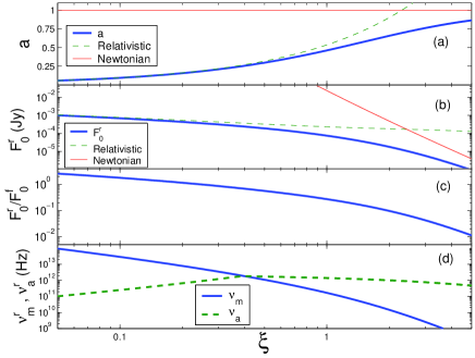
Figure 1: The parameter, $a$ and various break frequencies and flux densities as functions of $\xi$. (a): The parameter $a$ according to Eq. (11)(thick line), and its relativistic (dashed line) and Newtonian (thin line) approximations. (b): $F_{0}^{r}$ according to Eq. (6 & 13) when $a$ is calculated according to Eq. (11)(thick line), and when the relativistic (dashed line) or Newtonian (thin line) approximation of $a$ is taken. The physical parameters considered here are similar to these considered in panel d. (c): The ratio between the RS peak flux and the FS flux at the same time. $\epsilon_{e}$ and $\epsilon_{B}$ are assumed to be similar in the RS and the FS. (d): The synchrotron (solid line) and the self absorbtion (dashed line) frequencies of the RS emission at $t_{0}$. The parameters considered here are: $E_{52}=1$, $\epsilon_{e}=0.1$, $\epsilon_{B}=0.01$, $n=1$, $p=2.5$, $t_{0}=100$sec and $z=1$ ($D_{28}=1$).

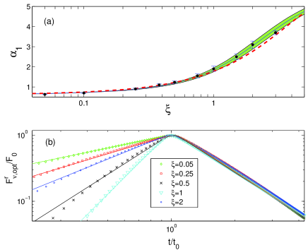
Figure 2: Results of detailed hydro+synchrotron numerical simulations. (a): $\alpha_{1}(\xi)$ as estimated by the mean value of $dlog(F_{\nu,opt}^{r})/dlog(t)$ at $t_{0}/2<t<t_{0}$, according to Eqs (14,15) (thin line), according to Eq. (4) (dashed line) and according to the numerical simulations (dots). The standard deviation of $dlog(F_{\nu,opt}^{r})/dlog(t)$ at $t_{0}/2<t<t_{0}$ is depicted by the shaded area (Eqs 14,15) and the error bars (numerical simulations). (b): Five numerical (normalized) optical light curves with various $\xi$ values, and their best fits according to Eq (2) (see sec. 4).

4 Numerical Simulations and Inhomogeneous Shells

The analytic calculations presented above include several approximations. In order to verify the accuracy of the analytic calculations we carried out detailed numerical simulations (Nakar & Granot 2004) of the early afterglow emission. We use these simulations to determine numerical correction factors, denoted ${\cal N}_{X}$, for the analytic calculations. The hydrodynamics simulations were done using a one dimensional Lagrangian code that was provided to us generously by Re’em Sari and Shiho Kobayashi (KS00). The synchrotron radiation code is described in Nakar & Granot (2004). This code provides an accurate synchrotron light-curve and spectrum, taking into account the realistic hydrodynamical profile of the emitting region, the exact heating and cooling history of the electrons and the precise photons arrival time to the observer from each radiating element.

We have carried the simulations for a range of parameters with $0.05\leq\xi\leq 3$. Using these simulations we obtain numerical corrections coefficients and determine the accuracy of the analytic estimates of $t_{0}$, $F_{0}^{r}$, $F_{\nu,opt}^{f}$ and $\alpha_{1}$. We find that when including the numerical correction factors (that range from 0.2 to 1.4), Eq.(1) for $t_{0}$ is accurate up to 10% while Eq.(6) (for $F_{\nu,opt}^{r}$) and the expression for $F_{\nu,opt}^{f}$ are accurate up to a factor $2$. The sharpness parameter $s$ was not considered before, and we find its value numerically. We find that if the shell is homogenous the peak is very sharp, $s\approx 10$, regardless of the value of $\xi$. Fig. 2b depicts five numerical light curves with $0.05\leq\xi\leq 2$, and their best fits according to Eq.(2). In all these fits $F_{0}$ is within factor of $2$ of Eq.(6), $t_{0}$ is within 10% of Eq.(1), $\alpha_{1}$ is within the spread of Eq.(4) (the shaded area in Fig. 2a), $\alpha_{2}\approx-2$ and $s\approx 10$.

So far we have considered homogeneous shells. Clearly, the light curve resulting from an inhomogeneous shell would depend on the shell’s profile. To investigate partially the effect of inhomogeneity, we have carried out numerical simulations of shells with linear Lorentz factor profile ($\delta\Gamma_{o}=1.6$) and a constant energy per a rest frame length interval. The value of $\xi$ varied between $0.05$ and $1$ where $\Gamma_{o}$ is taken as the mean value of the initial Lorentz factor. As expected in all the cases we find $\alpha_{2}\approx-2$ (which indicate that also the radio emission should be insensitive to the shell’s initial profile) and a sharp decrease in $s$ when $\xi\approx 1$ ($s\approx 1$ compared to $s\approx 10$ in the homogenous case). $F_{0}^{r}$, $t_{0}$ and $\alpha_{1}$ are similar to the values obtained in the homogenous case (a maximal difference of a factor of 1.5 between the homogeneous and inhomogeneous cases). These results make us confidant that the solution we present here for homogenous shell is generic and applicable also for inhomogeneous shells (at least as long as $\delta\Gamma_{o}$ is not much greater than $1$, and the Lorentz factor profile rises monotonically and regularly).

Finally we discuss briefly two caveats, which may arise naturally in a baryonic relativistic flow, and may alter the RS emission and produce a non-generic RS optical light curve. The first caveat is a slow tail of the wind with a small but not negligible, amount of energy (compared to the total energy of the wind). Such a tail may results from the adiabatic cooling of the wind after the phase of the prompt $\gamma$-rays emission, during which the wind must be hot. In this case the peak may be obtained before the RS finishes crossing the shell. Therefore the decay after the peak is expected to be shallower then the generic value of $-2$ (even for several orders of magnitude in time), becoming gradually steeper until the generic value is obtained . The second caveat is a highly irregular density profile. Such profile may result from a highly irregular ejection process in the source, as expected in the internal shocks scenario when a burst is highly variable. Since a hydrodynamic evolution smoothes the pressure and the velocity profiles, but not the density profile, such irregularities are expected to be carried by the flow also to the RS phase. If these irregularities in the density profile are large enough, they are expected to be reflected in the RS optical light curve during its rising phase and before its decay reaches the asymptotical value. Thus, a detailed observations of this phase may reveal the exact profile of the ejecta, and maybe even be used to test the internal shocks model (as the density profile in the flow is expected to reflect the light curve produced by internal shocks). Practically, if the early afterglow light curve is highly irregular, with no underlying power-law, then the analysis method described here is not applicable, and a theory that describes highly inhomogeneous RS is required. Note, however, that if the asymptotic value of the decay is reached soon after the peak, the tests of the RS emission (Eqs. 3 & 9) are still applicable.

Table 1: The Break Frequencies and Maximal Flux Densities

	value at $t=t_{0}$	$A_{x}^{x}(\xi)$	at $t<t_{0}$	$t>t_{0}$
${\nu_{m}^{r}}$	${2\cdot 10^{11}Hz(1+z)^{-\frac{1}{4}}\overline{\epsilon}_{e}^{\;2}\epsilon_{B-2}^{\frac{1}{2}}n^{\frac{1}{4}}E_{52}^{\frac{1}{4}}t_{0,2}^{-\frac{3}{4}}\overline{A}_{\nu,m}^{\;r}(\xi)}$	${a^{8}h_{a}^{-2}\xi^{-7.5}b_{\xi}^{3/4}}$	${\propto f^{2}a^{8}h_{a}^{-2}}$	${-1.5}$
${\nu_{c}^{r\;*}}$	${1\cdot 10^{17}Hz(1+z)^{-1/2}\epsilon_{B-2}^{-3/2}n^{-1}E_{52}^{-1/2}t_{0,2}^{-1/2}\overline{A}_{\nu,c}^{\;r}(\xi)}$	${a^{-4}\xi^{3}b_{\xi}^{-3/2}}$	${\propto f^{-2}a^{-4}b_{\xi}^{-2}}$
${\nu_{a}^{r\;\dagger}}$	${(5p+2)10^{12}Hz(1+z)^{-\frac{2}{5}}\overline{\epsilon}_{e}^{\;-1}\epsilon_{B-2}^{1/5}n^{\frac{2}{5}}E_{52}^{\frac{2}{5}}t_{0,2}^{-\frac{3}{5}}\overline{A}_{\nu,a}^{\;r}(\xi)}$	${a^{-8/5}h_{a}\,\xi^{12/5}b_{\xi}^{3/5}}$	${\propto f^{-1}a^{-8/5}h_{a}}$	${-0.55}$
${\nu_{a}^{r\;\dagger\dagger\dagger}}$	$(p-0.8)10^{13}Hz\left[(1+z)^{-\frac{p+6}{8}}\overline{\epsilon}_{e}^{\;p-1}\epsilon_{B-2}^{\frac{p+2}{4}}(nE_{52})^{\frac{p+6}{8}}t_{0,2}^{-\frac{3p+10}{8}}a^{4p}h_{a}^{\,1-p}\xi^{\frac{6-15p}{4}}b_{\xi}^{\frac{3p+10}{8}}\right]^{\frac{2}{p+4}}$		$\propto\left[\left(\frac{f}{h_{a}}\right)^{p-1}a^{4p}\right]^{\frac{2}{p+4}}$	${-1}$
${F_{\nu,b}^{r}}$	${250mJy(1+z)^{-\frac{5}{8}}\epsilon_{B-2}^{1/2}n^{\frac{3}{8}}E_{52}^{9/8}t_{0,2}^{-3/8}D_{28}^{-2}\overline{A}_{F,b}^{\;r}(\xi)}$	${a^{2}\xi^{-3/4}b_{\xi}^{3/8}}$	${\propto fa^{2}}$	${-0.95}$
${\nu_{m}^{f}}$	${1\cdot 10^{16}Hz(1+z)^{1/2}\overline{\epsilon}_{e}^{\;2}\epsilon_{B-2}^{1/2}E_{52}^{1/2}t_{0,2}^{-3/2}\overline{A}_{\nu,m}^{\;f}(\xi)}$	${a^{4}\xi^{-3}b_{\xi}^{3/2}}$	${\propto a^{4}}$	${-1.5}$
${\nu_{a}^{f\;\dagger}}$	${3GHz(1+z)^{-1}\overline{\epsilon}_{e}^{\;-1}\epsilon_{B-2}^{1/5}n^{3/5}E_{52}^{1/5}\overline{A}_{\nu,a}^{\;f}(\xi)}$	${a^{2/5}\xi^{-3/10}}$	${\propto f^{3/10}a^{2/5}}$	${0}$
${\nu_{a}^{f\;\dagger\dagger}}$	${0.6GHz(1+z)^{-\frac{1}{2}}\epsilon_{B-2}^{6/5}n^{\frac{11}{10}}E_{52}^{7/10}t_{0,2}^{-1/2}\overline{A}_{\nu,a}^{\;f}(\xi)}$	${a^{\frac{22}{5}}\xi^{-\frac{33}{10}}b_{\xi}^{\,\frac{3}{2}}}$	${\propto f^{\frac{13}{10}}a^{\frac{22}{5}}b_{\xi}}$	${-0.5}$
${F_{\nu,b}^{f}}$	${1.5mJy(1+z)^{-1}\epsilon_{B-2}^{1/2}n^{1/2}E_{52}D_{28}^{-2}\overline{A}_{F,b}^{\;f}(\xi)}$.	${a^{2}\xi^{-3/2}}$	${\propto f^{3/2}a^{2}}$	${0}$

Notations - ${\bf\epsilon_{e},\,\epsilon_{B}}$: the fraction of the internal energy in relativistic electrons and magnetic field respectively; ${\bf p}$: the electrons spectral index; ${\bf D}$: proper distance to the burst; $\overline{\epsilon}_{e}\equiv 30\epsilon_{e}(p-2)/(p-1)$; $b_{\xi}\equiv(1+{\cal N}_{t}0.5\xi^{3/2})$; $h_{a}\equiv a^{2}+1.5a+1$; $\overline{A}_{x}^{x}(\xi)\equiv A_{x}^{x}(\xi)/A_{x}^{x}(1)$

Using the table - $F_{\nu}(\nu)$ is found according the maximal flux, $F_{\nu,max}$, the values of the break frequencies and the spectral power law indices between them. All these vary between the different cases, where at each case $F_{\nu,max}$ is at a different break frequency:
$\nu_{m}<\nu_{a}<\nu_{c}$ (generic case): $F_{\nu,max}(\nu=\nu_{a})=F_{\nu,b}(\nu_{a}/\nu_{m})^{(1-p)/2}$; Power law indices: $2<\nu_{m}<2.5<\nu_{a}<(1-p)/2<\nu_{c}<-p/2$
$\nu_{a}<\nu_{m}<\nu_{c}$: $F_{\nu,max}(\nu=\nu_{m})=F_{\nu,b}$ ; Power law indices: $2<\nu_{a}<1/3<\nu_{m}<(1-p)/2<\nu_{c}<-p/2$
$\nu_{a}<\nu_{c}<\nu_{m}$: $F_{\nu,max}(\nu=\nu_{c})=F_{\nu,b}$ ; Power law indices: $2<\nu_{a}<1/3<\nu_{c}<-1/2<\nu_{m}<-p/2$
Column (2): The values at $t=t_{0}$. Column (3): The dependance at $t\leq t_{0}$ on $\xi$. Column (4): The evolution at $t<t_{0}$ can be found using this column and Eq. (14) (see sec. 3). Column (5): The approximated power-law indices at $t>t_{0}$, these values are uncertain by at least $\pm 0.05-0.1$ (see KS00). The values are calculated using the hydrodynamics of Eqs. (12, 16) ($t<t_{0}$) and KS00 ($t>t_{0}$), and the radiation calculations described in Sari, Piran & Narayan (1998), Granot, Piran & Sari (1999) and Granot & Sari (2001).
${}^{*}\nu_{c}^{f}=\nu_{c}^{r}$ at $t<t_{0}\;\;\;\;\;\;\;\;\;^{\dagger}\;\nu_{a}<\nu_{m}<\nu_{c}\;\;\;\;\;\;\;\;\;^{\dagger\dagger}\nu_{a}<\nu_{c}<\nu_{m}\;\;\;\;\;\;\;\;\;^{\dagger\dagger\dagger}\nu_{m}<\nu_{a}<\nu_{c}$

5 Conclusions

We have suggested here a parametrization of the early optical emission, as a broken power law with five parameters. We have calculated the values of these parameters for a RS produced by the interaction of baryonic wind with a circum burst ISM. Our main conclusions are: (i) The optical decay, ($\alpha_{2}\approx-2$) and the consistency between the peak time and flux of the optical and the radio (Eq. 2) are robust features of a RS emission in an ISM environment over a large range of initial parameters. Observations of an early optical emission with these features would suggest that: a) A significant fraction of outflow energy is baryonic . b) The circum-burst medium is an ISM like. c) The RS emission is dominant over other possible sources of optical flash. (ii) The values of the observables before the optical peak depend strongly on the strength of the shock, $\xi$, and can be used to pin down the initial conditions of the flow. (iii) The combination of optical flash and radio flare may also constrain the microscopic parameters in the emitting region.

In addition to the specific optical predictions we presented detailed analytical results of the expected emission over the whole spectrum. The advantages of these calculation over previous ones are that they do not make any approximation on the strength of the RS (i.e. relativistic or Newtonian), and that they are confirmed (and corrected) by numerical simulations. The conclusions of these calculations are: (i) Previous calculations overestimated the intensity of the optical flash. Most pronounced is the Newtonian approximation for $\xi\approx 1$ that overestimate the optical flash by up to three orders of magnitude. (ii) An optical flash brighter than $15$th mag is expected in some but not in all GRBs. A GRB with typical parameters and moderate energy ($E_{52}=1$), is expected to produce a maximal flux of $R_{mag}\sim 17-19$ when the RS is mildly relativistic ($\xi\approx 1$). (iii) Over some reasonable range of the parameters space the FS emission dominates at all times. (iv) When the RS is relativistic ($\xi\ll 1$) most of the emission is released in the optical. When $\xi$ increase, the emission is shifted to lower energy bands but it does not reaches the radio, as $\nu_{a}$ in this case is $\sim 10^{12-13}$Hz. These results suggest a solution to the “lack” of optical flashes. Only a fraction of the flashes is expected to be bright enough for detection in the current observations, and in some cases an FS emission is expected to dominate from the beginning.

We thank R. Sari and S. Kobayashi for providing us with their relativistic hydrodynamics code and J. Granot, P. Kumar, R. Mochkovitch, F. Daigne and E. Rossi for helpful discussions. The research was supported by the US-Israel BSF and by EU-RTN: GRBs - Enigma and a Tool. EN is supported by the Horowitz foundation and by a Dan David Prize Scholarship 2003.

References

- [] Beloborodov, A. M., 2002, ApJ, 565, 808
- [] Beuermann et al., 1999, A&A, 352, L26
- [] Chevalier, R. A. & Li, Z. Y., 2000, ApJ, 536, 195
- [] Fan, Y., Dai, Z., Huang, Y. & Lu T., 2002, ChJAA, 2, 449
- [] Fox et al., 2003a, ApJ, 586, L5
- [] Fox et al., 2003b, Nature, 422, 284
- [] Granot, J., Piran T. & Sari, R., 1999, ApJ, 527, 236
- [] Granot, J. & Sari, R., 2001, AAS, 34, 575
- [] Klotz, A., Atteia, J. L. & Boer, M., 2003, GCN circ. 1961
- [] Kobayashi, S., 2000, ApJ, 545, 807
- [] Kobayashi, S. & Sari, R., 2000, ApJ, 542, 819 (KS00)
- [] Kobayashi, S. & Zhang, B., 2003a,ApJ, 582 ,L75
- [] Kobayashi, S. & Zhang, B., 2003b, ApJ, 597, 455
- [] Kobayashi, S., Mészáros, P. & Zhang, B., 2004 ApJ, 601, L13
- [] Kumar P. & Panaitescu, A., 2003, MNRAS, 346, 905
- [] Mészáros, P. & M.J. Rees, 1997,ApJ, 476, 232
- [] Mészáros, P. & M.J. Rees, 1999, MNRAS, 306, L39
- [] Mészáros, P., Ramirez-Ruiz, E. & Rees, M. J., 2001, ApJ, 554, 660
- [] Nakar, E. & Granot, J., 2004 in preperation
- [] Nakar, E. & Piran, T., 2004, astro-ph/0405473
- [] Rykoff, E. S. et al., 2004, ApJ, 601, 1013
- [] Rykoff, E. & Smith, D., 2002, GCN circ. 1480
- [] Sari, R. & Piran, T., 1995, ApJ, 455, L143 (SP95)
- [] Sari, R. & Piran, T., 1998, in Gamma-Ray Bursts: 4th Huntsville Symposium, ed. C. Meegan, R. Preece and T. Koshut, 662
- [] Sari, R. & Piran, T., 1999b, ApJ, 517, L109
- [] Sari, R. & Piran, T., 1999a, ApJ, 520, 641
- [] Sari, R., Piran, T., & Narayan, R., 1998, ApJ, 497, L17
- [] Sari, R. & M esz aros, P., 2000, ApJ, 535, L33
- [] Soderberg, A. M. & Ramirez-Ruiz, E., 2003a, MNRAS, 345, 854
- [] Soderberg, A. M. & Ramirez-Ruiz, E., 2003b, MNRAS, 330, L24
- [] Thompson, C. & Madau, P., 2000, Apj 538, 105
- [] Torii, K., 2003a, GCN circ. 2381
- [] Torii, K., 2003b, GCN circ. 2253
- [] Wang, X. Y., Dai, Z. G. & Lu, T. 2000, MNRAS, 319, 1159
- [] Weidong L., Alexei V., Ryan C. & Saurabh J., 2003, ApJ, 586 L9
- [] Williams, G.G., Park, H. S., & Porrata, R., 1999, GCN circ. 437
- [] Wu, X., Dai, Z., Huang, Y., & Lu, T., 2003 MNRAS, 342, 1131
- [] Zhang, B., Kobayashi, S. & Mészáros, P., 2003, ApJ, 595, 950