SN1987A and the properties of the neutrino burst

Abstract

We reanalyze the neutrino events from SN1987A in IMB and Kamiokande-II (KII) detectors, and compare them with the expectations from simple theoretical models of the neutrino emission. In both detectors the angular distributions are peaked in the forward direction, and the average cosines are 2 sigma above the expected values. Furthermore, the average energy in KII is low if compared with the expectations; but, as we show, the assumption that a few (probably one) events at KII have been caused by elastic scattering is not in contrast with the ’standard’ picture of the collapse and yields a more satisfactory distributions in angle and (marginally) in energy. The observations give useful information on the astrophysical parameters of the collapse: in our evaluations, the mean energy of electron antineutrinos is $\langle E\rangle=12-16$ MeV, the total energy radiated around $(2-3)\times 10^{53}$ erg, and there is a hint for a relatively large radiation of non-electronic neutrino species. These properties of the neutrino burst are not in disagreement with those suggested by the current theoretical paradigm, but the data leave wide space to non-standard pictures, especially when neutrino oscillations are included.

I Motivations and context

The detection of neutrinos from SN1987A marked the beginning of (extra)galactic neutrino astronomy IMBdata87 ; IMBdata ; KIIpaper87 ; KIIpaper ; Baksan87 ; MontBlanc (see also Olga ; raffelt ; Koshiba for comprehensive reviews of SN1987A observations). The observations of Kamiokande have been mentioned and recognized in the 2002 Nobel prize for Physics. However, when one studies the data, one meets a number of surprising, unexpected or even puzzling features. Let us recall which are the main ones.
(1) The angular distributions of the events seen at Kamiokande-II (KII) and at Irvine-Michigan-Brookhaven (IMB) are more forward-directed than expected, for instance, the average cosines of the polar angles are $\langle\cos\theta^{\rm KII}\rangle\sim 0.3$ and $\langle\cos\theta^{\rm IMB}\rangle\sim 0.5$.
(2) Also, the energy distribution of these two detectors seems not to be perfectly in agreement. In particular, $\langle E_{vis}^{\rm KII}\rangle$ is half of $\langle E_{vis}^{\rm IMB}\rangle$ (about $30$ MeV), that is, a very marked difference even taking into account the different performances of the detectors.
(3) Even the time distribution of the events in the two detectors looks to be different. However, when data are combined the distribution in time does not contradict the current picture of a ‘delayed explosion’ according to Lamb and Loredo analysis LambLoredo .
(4) The Mont Blanc events MontBlanc occurred $4.5$ hours before the other ones. This led some Authors to consider two-stage scenarios for the collapse nb1 .
In this work, we will focus on the discussion of the first issue and will stress the connections with the second one. More in general, we believe that these data raise several important questions that deserve attention, for instance: How likely is that the anomalies in the distributions are due to fluctuations, and in particular, how significant is the hint for some feature in the angular distributions? What can we learn (and what we can exclude) on the nature and the properties of the stellar collapse from these observations?

A number of recent facts, beside the general considerations exposed above, testify the interest in having a fresh look at the SN1987A data: (a) several experimental evidences (in particular SuperKamiokande ; SNO ; Kamland ) strongly suggest that SN1987A neutrinos oscillated in flavor; (b) the expectations of the emitted neutrino radiation has been recently reconsidered Janka , suggesting a new paradigm for the distribution of neutrinos and antineutrinos; (c) there have been improvements in the description of the cross section of

$$\bar{\nu}_{e}\;p\to e^{+}\;n,\ \ \mbox{IBD reaction (from `inverse beta decay')}$$ (1)

in the energy range relevant for supernova neutrinos beacom ; vissani . Moreover, it is correct to recall that we do not understand yet the theory of core collapse supernovae, and therefore one could argue that we miss the most important ingredient for a proper interpretation. However, a reasonable working hypothesis is to describe the emitted neutrino radiation by a model with few parameters, suggested by the ‘delayed explosion’ scenario proposed in del , see JANKA for a recent report. This is the point of view we will adopt in a large part of the present investigation.

We will describe and motivate in the rest of this Section what we assume (based on expectations and observations) as a reference neutrino flux. We will discuss a standard (but updated) comparison of observations and expectations in Section 2, based on IBD hypothesis (see below), that will permit to further define the parameters of the model of neutrino emission. In Section 3, we will use this model to analyze the angular features of the spectra, state the situation quantitatively, and consider a few alternatives to improve the agreement with the data. We summarize the results obtained in the last Section.

I.1 Neutrino flux

A simple model of the fluxes Janka of supernova neutrinos attributes the following spectra (with three different average energies $E_{0}$) to any species $\nu_{e}$, $\nu_{\bar{e}}$ or $\nu_{x}$–$x$ being any among muon and tau (anti)neutrinos:

$$\Phi_{i}(E)=\frac{{\cal E}_{i}}{4\pi D^{2}}\ \frac{N}{E_{0}^{2}}\ z^{\alpha}e^{-(\alpha+1)z},\ \ z=E/E_{0}$$ (2)

where $i=e,\bar{e},x$ and $N={(\alpha+1)^{\alpha+1}}/{\Gamma(\alpha+1)}$. The total fluence at the detector is $\int E\Phi_{i}(E)dE={{\cal E}_{i}}/4\pi D^{2}$, thus ${\cal E}_{i}$ is the amount of irradiated energy in the neutrino species $i$ (the flux is supposed to be emitted isotropically) and $D$ the SN-detector distance. Numerical calculations find that the time integrated flux $\Phi$, usually called ‘fluence’, is rather well described by this ansatz; in particular, the deviations from a thermal shape are not large, and can be described as we do here by setting $\alpha=3$ for all neutrino species ($\alpha=2$ amounts to a Maxwell-Boltzmann distribution). Finally, the meaning of $E_{0}$ is just the average energy of the species considered (we will take $E_{0}=\langle E_{\bar{e}}\rangle$ in the following).

The total energy emitted in neutrinos can be estimated by simple considerations. In fact, the total gravitational energy irradiated is ${\cal E}_{B}\sim 3G_{N}M_{ns}^{2}/5R_{ns}$, and using for the neutron star a mass of $M_{ns}=(1-2)M_{\odot}$ and a radius of $R_{ns}=20\mbox{ km }(M_{\odot}/M_{ns})^{1/3}$, we get ${\cal E}_{B}\sim(1-5)\times 10^{53}$ erg. The amount of energy that goes in the specific flavors is uncertain. Since ${\cal E}_{e}$ is not very important for the observed signal (see below), we will always set ${\cal E}_{e}={\cal E}_{\bar{e}}$, unless stated otherwise. Instead, we will distinguish three cases for the emitted energy ${\cal E}_{x}$ (assumed to be equal for $\nu_{\mu}$, $\nu_{\bar{\mu}}$, $\nu_{\tau}$ and $\nu_{\bar{\tau}}$, so that ${\cal E}_{B}={\cal E}_{e}+{\cal E}_{\bar{e}}+4{\cal E}_{x}$) that, as we will see, plays a more important role:

1. ${\cal E}_{x}={\cal E}_{\bar{e}}$: This is the so-called ‘equipartition’, often adopted in theoretical analyses.

2. ${\cal E}_{x}={\cal E}_{\bar{e}}/2$: This is the case when a large part of the radiation goes in electron neutrinos.

3. ${\cal E}_{x}=2{\cal E}_{\bar{e}}$: Finally, in this case most of the radiation goes in muon or tau neutrinos.

The average energies are important parameters. $\langle E_{x}\rangle$ is greater than $\langle E_{\bar{e}}\rangle$, but the amount of hierarchy found in modern calculations is not very large. A typical ratio is in the range $1-1.2$. In the following, we will assume (unless stated otherwise) $\langle E_{x}\rangle=1.1\langle E_{\bar{e}}\rangle$. The average energy of the electron neutrinos $\langle E_{e}\rangle$ instead is not of crucial importance for the observed signal. It can be evaluated by prescribing a condition on the emitted lepton number $\Delta L_{e}=N(\nu_{e})-N(\bar{\nu}_{e})$ where $N(\nu_{e})={\cal E}_{e}/\langle E_{e}\rangle$ and similarly for the antineutrinos; we will assume that the electrons contained in one solar mass of iron are converted in neutrinos.

The crucial parameters needed to describe the neutrino signal are the antineutrino average energy,

$$E_{0}\equiv\langle E_{\bar{e}}\rangle=12-18\ {\rm MeV}\;\;\ \ \ \mbox{(expected)}$$ (3)

and the total energy irradiated in antineutrinos

$${\cal E}_{\bar{e}}=(2-10)\times 10^{52}\ {\rm erg}\ \ \ \ \ \ \ \mbox{(expected)}$$ (4)

Both of them have considerably uncertainties, especially the second one. For this reason, the uncertainty in the distance of the supernova is usually considered unimportant; here, we will assume $D=52$ kpc, and discuss this point later.

I.2 Impact of neutrino oscillations

Motivated by the solar and atmospheric results, we assume that the three neutrinos $\nu_{e}$, $\nu_{\mu}$ and $\nu_{\tau}$ have mass and mix among them. Following simple minded theoretical expectations, we will further assume in most of this paper that the heaviest state is separated by $\Delta m^{2}_{31}\approx 2.5\times 10^{-3}$ eV² from the other two, whose splitting is $\Delta m^{2}_{21}\approx 7\times 10^{-5}$ eV². The known mixing angles are $\theta_{23}\approx 45^{\circ}$, $\theta_{12}\approx 34^{\circ}$, while $\theta_{13}$ is unknown but presumably it is not very small (we take $\approx 6^{\circ}$ when needed, but its impact on the oscillations is usually of minor importance). With these parameters, the emitted fluxes from SN1987A, described in Sect.I.1, should be modified to account for the MSW effect in the star raffelt_neubig ; dutta ; fogli ; burrows_osc ; smirnov (among first papers on the topic, we recall Mikheev_smirnov ; Kuo ; Minakata ; Arafune ; Notzold ):

$$\left\{\begin{array}[]{l}\Phi_{e}\to P_{ee}\Phi_{e}+(1-P_{ee})\Phi_{x}\\ \Phi_{\bar{e}}\to P_{\bar{e}\bar{e}}\Phi_{\bar{e}}+(1-P_{\bar{e}\bar{e}})\Phi_{x}\end{array}\right.$$ (5)

where the two probabilities of survival are $P_{\bar{e}\bar{e}}=\cos^{2}\theta_{12}\approx 0.7$ and $P_{ee}=\sin^{2}\theta_{13}\approx 0$. (We will discuss other possibilities, as a very small $\theta_{13}$, or an ‘inverted’ mass hierarchy, in Sect.III.4.) The MSW effect of the Earth modifies $P_{\bar{e}\bar{e}}$ by a minor amount nb2 .

Two remarks are in order: (1) It is difficult to conceive that oscillations did not occur; for instance, the MSW effect related to solar $\Delta m^{2}$ happened unless there was a drastic modification of the mantle of the star for densities around 10 gr/cc, which seems unlikely. (2) The effects for $\bar{\nu}_{e}$ are of about 30 %, while those for $\nu_{e}$ can be much larger; for instance, in the framework described above, the observed $\nu_{e}$ flux corresponds almost exclusively to emitted $\nu_{\mu}$ or $\nu_{\tau}$. This is the reason why ${\cal E}_{x}$ has an important role for the signal seen in terrestrial detectors.

II The IBD hypothesis

In the model previously described and with the expected values of the parameters, it is a fact that most of the events expected at KII and IMB are due to the inverse beta decay process. This is the reason why several analyses adopted the simplifying hypothesis that all events come from IBD (see e.g. janka_hille ). We begin by repeating such a more-or-less standard analysis, with three specific aims: (1) stressing observables with a clear physical meaning (rather than attempting a global analysis of the data); (2) discussing how the various data fit in the theoretical picture; (3) getting more specific values of the parameters of neutrino emission. The calculations of the expectations are quite simple. In a detector with $N_{p}$ protons and with detection efficiency $\epsilon(E)$ (function of the positron energy) one integrates the differential event rate

$$\frac{dN_{ibd}}{dE_{\nu}dE}=N_{p}\;\epsilon(E)\;\Phi_{\bar{e}}(E_{\nu})\;\frac{d\sigma_{ibd}}{dE}(E_{\nu},E)$$ (6)

over the allowed range, obtaining the value of the observable of interest–e.g., the visible energy in Čerenkov detectors $E_{vis}=E$ (note that the fluence $\Phi$ should be thought as differential in the transversal surface and in $E_{\nu}$). In Figure 1, we show the value of two simple but interesting observables: the mean energy and the number of events. In this Figure, the effect of varying $\langle E_{\bar{e}}\rangle$, $\langle E_{x}\rangle$ and ${\cal E}_{x}$ in certain ranges are illustrated. For IMB, we reduced the expected number of events by 13% to take into account the dead-time occurred during the detection of the burst IMBdata . Let us comment the results in some detail:

Average visible energy

This observable has the advantage of being independent of the total energy emitted, and of having relatively small errors:

$$\delta E_{vis}=\sqrt{\frac{\langle E^{2}_{vis}\rangle-\langle E_{vis}\rangle^{2}}{N}}=\left\{\begin{array}[]{l}2.4\ \mbox{MeV at KII}\\ 2.6\ \mbox{MeV at IMB}\end{array}\right.$$ (7)

in the IBD hypothesis $E_{vis}$ is the energy released by the positron. While IMB points to a range of values nicely consistent with expectations, compare with eq.(3), the data of KII point to somewhat lower values. Note that we discard from the analysis the sixth event of KII, since it has $N_{hit}=16$, below the threshold $N_{hit}=20$ of software analysis KIIpaper . Indeed, it should be remarked that the lower energy events are those for which pollution from background is more likely; in particular, in the window of 12 sec in which the supernova neutrinos have been detected at KII, we estimate an average of about 2 background events KIIpaper . From Figure 1, one sees that the impact of a variation of $\langle E_{x}\rangle$ and ${\cal E}_{x}$ on the expectation for the average visible energy is not large.

Number of events

The observables $N^{\rm KII}=11$ and $N^{\rm IMB}=8$ have large Poisson errors, but permit to estimate the energy emitted from the supernova (whereas, the previous observable is not useful for this purpose). In the two plots on the right of Figure 1, the energy emitted in any species of neutrino is chosen by default to be $4\times 10^{52}$ erg. We see that the agreement with the expectations is not bad, and also that the impact of a variation of ${\cal E}_{x}$ is not fully negligible. This is easy to understand and to keep into account; indeed, the signal scales roughly as $0.7{\cal E}_{\bar{e}}+0.3{\cal E}_{x}$, thus a variation in ${\cal E}_{x}$ can be well simulated by a variation of the total emitted energy.

Summary

Using these results as a guide, we further specify the parameters of the model and assume

$$E_{0}\equiv\langle E_{\bar{e}}\rangle=14~{}\mbox{MeV},\ \ \ {\cal E}_{\bar{e}}=4\times 10^{52}\ \mbox{erg}$$ (8)

These values should be thought as compromises between contrasting needs. For instance, KII energy spectra suggest lower values of $E_{0}$, whereas in order to reproduce the number of events at central values, we need $E_{0}\sim 18$ MeV and ${\cal E}_{\bar{e}}=3\times 10^{52}$ erg. In view of this situation, we find it reassuring that the values shown in eq.(8) are in accordance with the expectations from a ‘standard’ collapse (as defined in eqs. (3) and (4)).

We conclude this first part of the analysis reassessing that within the ‘standard’ model of the collapse and with the parameters of eq. (8), the observed average visible energy at KII looks a bit small (see again Figure 1).

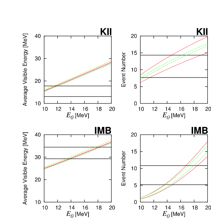
Figure 1: Comparison of observations (horizontal strips) and expectations calculated in the IBD hypothesis. The left panels show the average visible energy, the right ones the number of events. The upper panels are for KII, the lower ones for IMB. For any panel, we show 4 expectations curves. The continuos (red) ones correspond to a variation of the theoretical parameter ${\cal E}_{x}$ (=energy radiated in $\bar{\nu}_{\mu,\tau}$) in the range $(2-6)\times 10^{52}$ erg. The dashed ones (green) correspond to a variation of the theoretical parameter $\langle E_{x}\rangle$ (=average energy of the emitted $\nu_{\mu}$, $\nu_{\bar{\mu}}$, $\nu_{\tau}$ and $\nu_{\bar{\tau}}$) in the range $(1-1.2)\times E_{0}$.

III What is the meaning of the forward events?

Table 1: Approximate coefficients of the angular distributions for IBD using eq. (8).

	$a_{0}$	$a_{1}$	$a_{2}$
KII	0.499	0.030	0.003
IMB	0.495	0.104	0.014
IMB with bias	0.492	0.154	0.024

In this Section we study the angular distribution of the events from SN1987A. Thus, we select the events from the two water Čerenkov detectors operative at that time, and use the data from IMBdata for IMB, and those from KIIpaper for KII. Both angular distributions are rather forward-directed. To state this more precisely, we calculate the average angles: $\langle\cos\theta^{\rm KII}\rangle=0.29\pm 0.27$ and $\langle\cos\theta^{\rm IMB}\rangle=0.48\pm 0.34$. Here we have used a weighted average and the corresponding standard deviation errors.

Beyond the IBD hypothesis

We can compare the data with the expectations from the IBD hypothesis. Using parameterized angular distributions

$$dN/dz=a_{0}+a_{1}z+a_{2}z^{2},\ \ \ \mbox{where }z=\cos\theta\mbox{ and }a_{i}\mbox{ as in Tab.\ref{tab1}}$$ (9)

obtained from vissani we find that both central values are above the expected ones: 2.3$\sigma$ for IMB and 1.7$\sigma$ for KII. This conclusion is in agreement with beacom . In this study, we adopt the model defined in the previous Section with the parameters of eq. (8). We checked that a variation of these parameters is not crucial for the conclusions, while ${\cal E}_{x}$ is of greater importance. It is simple to explain the reason: The only type of events that is strongly forward (and thus is able to affect the angular shape of the distribution) are those from

$$\nu_{i}\;e\to\nu_{i}\;e,\ \ \ \mbox{ES reaction (from `elastic scattering'),}\ \ \ \ i=e,\bar{e},x$$ (10)

This reaction receives contributions from all neutrino types, and $\nu_{e}$ gives the largest one. But due to oscillations, eq. (5), the observed $\nu_{e}$ flux is originally due to $\nu_{x}$; this implies the relevance of ${\cal E}_{x}$, namely, the energy emitted in $\nu_{\mu,\tau}$. The hypothesis that one or more forward peaked elastic scattering events could be present in the data samples of IMB and KII has been already considered in the past, see e.g. spergel ; krauss ; LoSecco ; Olga ; MIK ; malguin . In this analysis, however, we update the angular distributions for IBD events and the model for neutrino emission, compare different statistical inferences and include oscillations with recently measured parameters.

Figure 2: Reconstructed angular distribution for elastic scattering events in KII.

Instrumental effects

A point to take into account is that the angular distributions (and in particular the one of ES) are modified in an important manner by instrumental effects. This is due to multiple scattering and limited angular resolution of the detectors, and it is called ‘smearing’ of the angular distributions. In order to account for this, we use the following distribution Danuta :

$$\rho_{sm}(\cos\theta_{s})d\cos\theta_{s}=N\,e^{-\theta^{2}_{s}/2\sigma_{s}^{2}}\,\sin\theta_{s}d\theta_{s}\,$$ (11)

where $\theta_{s}$ is the angle of smearing and $\sigma_{s}$ is a measure of the effect; $N$ in eq. (11) is just a normalization factor. For KII, where the smearing is slightly more important, we choose $\sigma_{s}$ in such a way that the mean angle $\overline{\theta}$ from (11) corresponds to the mean error ${\delta\theta}$ determined from the data KIIpaper . For the whole set of data we have $\delta{\theta}\sim 25^{\circ}$, while considering only data with $\theta\leq 30^{\circ}$ we find $\delta\theta\sim 18^{\circ}$. As a consequence we decide to study the two cases, when $\sigma_{s}=15^{\circ}$ and $\sigma_{s}=20^{\circ}$, for which $\overline{\theta}\sim 18^{\circ}$ and $\sim 25^{\circ}$, respectively. Based on similar considerations IMBdata we set $\sigma_{s}=16^{\circ}$ in IMB. Using eq. (11) and $\rho_{es}$ e.g. from bahcall we can determine the reconstructed angular distribution as follows:

$$\rho_{es}^{rec}({\bf n}\cdot{\bf m})=\int d^{2}{\bf p}\ \rho_{sm}({\bf m}\cdot{\bf p})\ \rho_{es}({\bf n}\cdot{\bf p})$$ (12)

where ${\bf n}$, ${\bf{m}}$ and ${\bf p}$ are unitary vectors for the SN, the reconstructed and the emitted direction respectively, ${\bf n}\cdot{\bf m}=\cos\theta$, ${\bf m}\cdot{\bf p}=\cos\theta_{s}$, ${\bf n}\cdot{\bf p}=\cos\theta\cos\theta_{s}+\sin\theta\sin\theta_{s}\cos\phi_{s}$, and $d^{2}{\bf p}=d\cos\theta_{s}d\phi_{s}/4\pi$ is an element of solid angle from which the signal receives a contribution. The reconstructed distributions we obtain for KII are plotted in Figure 2. Since the angular distribution $\rho_{es}$ of ES is rather narrow (especially when taking into account detector efficiencies) the reconstructed angular distribution of ES is mostly dictated by instrumental effects.

III.1 Angular distribution of IMB

The normalized positron angular distribution for inverse beta decay is usually taken in the simple approximation $dN/d\cos\theta=0.5+a\cos\theta$; in particular, in the IMB report IMBdata it is assumed $a\sim 0.07$. In the same paper it is pointed out that to account for the experimental polar-angle efficiency, one can introduce a 10 % angular bias. This is equivalent to replace $dN/d\cos\theta\rightarrow(1+0.1\cos\theta)\ dN/d\cos\theta$. We use the improved cross-section for IBD from vissani to determine the parameters $a_{i}$ ($i=0,1,2$) in Tab. 1, that enter in the angular distribution of eq.(9). We notice that $a_{i}$’s in Tab.1 do not depend significantly on the assumed mean energy $E_{0}$.

We have used eq. (9) to test the hypothesis the data from IMB come from IBD events, employing the Smirnov-Cramer-Von Mises (SCVM) statistics SCMtest . As shown in the left panel of Figure 3 the goodness of fit (g.o.f.) for this hypothesis is equal to 6.4%. The improved IBD angular distribution changes the previous result (4.5% IMBdata ) by only a small amount due to the poor statistics. However, the importance of using the improved angular distribution is evident when we compare the old significance without angular bias with the new one, since 1.5 % IMBdata increases to 4.2 %. In the same Figure we show the cumulative distribution in the hypothesis of having 1 ES event in IMB.

To study the possibility to have a small contribution of Elastic Scattering (ES) events in IMB and later in KII we have exploited the Maximum Likelihood (ML) method bookEML . In this framework the likelihood function is written:

$$L\left(\frac{n}{n_{obs}}\right)=\prod_{i=1}^{n_{obs}}\rho\left(\cos\theta_{i};\frac{n}{n_{obs}}\right)\,$$ (13)

where $n/n_{obs}$ is the parameter which measures the fraction of ES events, $n_{obs}$ being the total number of experimentally observed events for the SN. The angular distribution $\rho(\cos\theta_{i};n/n_{obs})$ can be written as $\rho(\cos\theta;n/n_{obs})=(n/n_{obs})\rho_{es}^{rec}(\cos\theta)+(1-n/n_{obs})\rho_{ibd}(\cos\theta)$, where $\rho_{es}^{rec}$ and $\rho_{ibd}$ are the angular distributions for ES and IBD, respectively. It turns out that in IMB the best-fit is found for $n/n_{obs}=0$. The effect of the smearing is not particularly important in IMB. In order to determine an upper limit on the likelihood parameter we have built a posterior probability distribution function (p.d.f.) by normalizing the likelihood function and considering a uniform prior p.d.f. which is equal to one for $n/n_{obs}\geq 0$, zero elsewhere. It turns out that $n/n_{obs}<0.12$ at 68.3% C.L., namely the IMB angular distribution admits one ES event at most.

Figure 3: Theoretical and experimental angular distributions in IMB (left panel) and KII (right panel). The 1 sigma range and the goodness of fit figures are also shown. For KII, we adopt $\sigma_{s}=15^{\circ}$.

Figure 4: Normalized likelihood function versus the fraction of expected ES events in KII. For the smearing of the angular distribution we show the cases $\sigma=20^{\circ}$ and $\sigma=15^{\circ}$.

III.2 Angular distribution of KII

As stated above we consider $n_{obs}$=11 out of 12 candidate events KIIpaper and assume the event number 6 due to background. In Figure 2 we show the reconstructed angular distributions for the cases $\sigma_{s}=15^{\circ}$ and $\sigma_{s}=20^{\circ}$. The smearing effect in KII plays an important role (without smearing, $\langle\theta\rangle=10^{\circ}$). Using the ML from eq. (13) we have computed the likelihood ratio $L(n/n_{obs})/L_{max}$ with $n=0,1,2,3$ to quantify the probability to have zero, one or more ES events on the basis of the angular distribution. In Figure 4 we show the normalized ML function against $n/n_{obs}$. Minimizing $-\ln L(n/n_{obs})$ the best-fit is found for $n/n_{obs}=0.35\pm 0.20$(1$\sigma$) for $\sigma_{s}=20^{\circ}$ and $n/n_{obs}=0.23^{+0.21}_{-0.18}$(1$\sigma$) for $\sigma_{s}=15^{\circ}$ . So, the ML test suggests that a few ES events are present in the KII dataset.

As for IMB we have exploited the SCVM test (see Figure 3). Moreover, we have worked out the probability to have $n=0,1,2,3$ ES scattering events using the expectations based on the SN model described above. For this latter case we have written the probability to have $n$ ES events out of a total of $n_{obs}$=11 as the product of two Poisson distributions, that is equal to:

$$P(n)=\frac{e^{-n_{exp}}}{n_{obs}!}\ n_{exp}^{\ n_{obs}}\times B_{p}(n,n_{obs})\,$$ (14)

where the first factor is a Poisson distribution with a mean value $n_{exp}=n_{es}+n_{ibd}$ and the second one a Binomial distribution with a trial probability $p=n_{es}/n_{exp}\sim 0.03$; for instance, for the equipartition scenario we found 11.9 IBD events and 0.39 ES events. (Incidentally, one should notice that the calculation of the ES number of events is very sensitive to the experimental efficiency at the lowest measurable energies). In Tab. 2 we summarize our results. Similar calculations were made for IMB.

Table 2: Expected probabilities that zero, one or more events in KII are due to ES, for $\sigma_{s}=15^{\circ}$ (upper part) and $\sigma_{s}=20^{\circ}$(lower part). The first line shows the a priori expectation from the model of eq.(8), while the second and the third line use the information from the observed angular distribution.

	$n=0$	$n=1$	$n=2$	$n=3$
from SN model	50.5%	38.9%	9.7%	0.9%
g.o.f. from SCVM	8.6%	26.7%	58.5%	81.4%
likelihood ratio $L(n)/L_{max}$	0.35	0.73	0.97	0.98
from SN model	52.3%	37.5%	9.2%	1.0%
g.o.f. from SCVM	8.6%	24.9%	53.8%	87.6%
likelihood ratio $L(n)/L_{max}$	0.14	0.39	0.69	0.92

III.3 Summary for the ‘standard’ scenario and remarks

It is instructive to compare here the outcomes of the two statistical tests we used: the Smirnov-Cramer-Von Mises (SCVM) and the maximum likelihood (ML). The comparison with the data follows completely different strategies: the ML method is ‘local’ in the sense that it profits of events that fall under the ES bell (of Fig.2), while the SCVM is ‘global’ in the sense that it tries to minimize the maximal distance between the theoretical curve and the observed one. For IMB the SVCM test suggests more elastic scattering events than the ML test does (the reason can be understood from the right-most part of figure 3a: the most forward event has polar angle $33^{\circ}\pm 15^{\circ}$, thus its central value is not forward enough to suggest an ES event). Instead, for KII the two tests give very similar indications.

Next, we take into account also the theoretical expectation on the number of ES events, and use it together with the results from the angular distribution. We combined the information from the SN model and that from the SCVM analysis in Tab. 2, multiplying the probabilities and normalizing the resulting distribution to one. The results for KII are shown in Tab. 3, and the combined probabilities are given for the case $\sigma=20^{\circ}$ (the case $\sigma=15^{\circ}$ gives about the same result). In particular, from Tab. 3 we see that one ES in KII can be accepted at about the same level we could accept zero events. Moreover, even the probability to have two ES events is indeed not negligible. Repeating the exercise for IMB, we find that at ‘equipartition’ (${\cal E}_{\bar{e}}={\cal E}_{x}$) the combined probability to have zero (one) events is 80 % (19.9 %).

Some remarks are in order.
(1) The data of KII show that the most directional events have energies above 20 MeV. Taking this experimental fact into account, we checked the probability to have events with $E_{e}\geq 20$ MeV for the three scenarios of SN considered. As shown in Figure 5 this probability is about 16%. So, it seems not unlikely nb5 from this point of view to have measured ES events with energies above 20 MeV.
(2) The presence of one or more ES events in KII dataset goes in the right direction to explain the disagreement between IMB and KII average energies. However the effect is admittedly small, since for instance 1 ES event that produces $20$ MeV of observable energy originates from a neutrino with larger energy, but just of $5$ MeV on average. If the number of ES events in KII is larger, this could become more important.

Figure 5: Expected energy distribution of scattering events in KII, for ${\cal E}_{x}=(0.5,1,2)\times{\cal E}_{\bar{e}}$. Also shown is the probability to have one event with energy larger than 20 MeV.

III.4 Speculations

Table 3: Relative percentage probabilities to have a given number of ES events in KII dataset, estimated from observed angular distribution and theoretical expectation on the fluxes, for 3 hypotheses on ${\cal E}_{x}$.

	$n=0$	$n=1$	$n=2$	$n=3$
${\cal E}_{x}={\cal E}_{\bar{e}}/2$	52.3%	37.5%	9.2%	1.0%
${\cal E}_{x}={\cal E}_{\bar{e}}$	40.0%	42.3%	15.3%	2.5%
${\cal E}_{x}=2\;{\cal E}_{\bar{e}}$	29.0%	43.6%	22.3%	5.1%

It is interesting to consider at this point some speculative scenarios, to investigate the question under which conditions we can increase the expected number of ES events:

• A distinguished astrophysical possibility is that there are main departures from a ‘standard’ collapse, and a large part of the emitted energy is not seen by inverse beta decay. Let us assume as an extreme case that the electron neutrinos have an average energy of $40$ MeV and carry an energy of $1.5\times 10^{53}$ erg nb6 . The calculation reveals that the increase is not much larger: In KII, we expect $N_{dir}=0.59$ rather than $N_{dir}=0.39$. The reason is simply that oscillations transform the $\nu_{e}$ into $\nu_{\mu}$ and $\nu_{\tau}$, and the interaction cross section of these neutrinos is smaller.

• Another possibility is to study which adjustment of the ‘standard’ scenario goes in the right direction. In particular, one can suggest that the $\nu_{x}$ are more energetic than what we assumed. This does not help for the number of events, but helps a bit to explain the fact that the directional events are among the most energetic ones.

• The uncertainties in oscillations provide us with another degree of freedom. It seems to us very difficult to avoid the occurrence of MSW oscillations completely, but if $\theta_{13}$ is very small, we could get $P_{ee}=0.3$. The result $P_{ee}=\sin^{2}\theta_{12}=0.3$ assumes that the mantle of the star at densities of about 10 gr/cc was not essentially modified by the pre-collapse events. The opposite case seems unlikely, but one could get $P_{ee}=1-\sin^{2}2\theta_{12}/2\sim 0.6$. However, this does not help to increase $N_{dir}$ with the ‘standard’ scenario, and it is of limited use to invoke non-standard scenarios with energetic $\nu_{e}$’s, since in this case the reaction with oxygen are also called into play, see Haxton and Burrows_gandhi . Another case arises if $\theta_{13}$ is ‘large’ when the neutrino mass spectrum is inverted, rather than ‘normal’ as considered previously in the text. In fact, in this hypothesis the IBD events are due to the flux $\Phi_{x}$, and the flux of $\nu_{e}$ (important for ES events) is $0.3\Phi_{e}+0.7\Phi_{x}$. Thus, we are interested to consider the possibility of a large ${\cal E}_{e}$ to increase the number of ES events, or the possibility that ${\cal E}_{e}>{\cal E}_{x}$, since in this way we reduce the number of IBD events more than the ES events.

• A more drastic attitude is to abandon completely the ‘standard’ idea of the collapse. A specific suggestion made in malguin is that a large amount of neutrino radiation comes from $\pi^{+}\to\mu^{+}\nu_{\mu}$ decay. The largest contribution to scattering events comes from the electron neutrinos, that, due to oscillations originate exactly from $\nu_{\mu}$ (in fact, due to the loop-induced difference of potential between $\tau$ and $\mu$ neutrinos $\nu_{\mu}\to\nu_{1}$ and a $\nu_{e}$ happens to be produced with probability $P_{\mu\to e}=0.7$). The $\nu_{\mu}$ are monochromatic with energy $29.8$ MeV. If the energy injected in $\nu_{\mu}$ is $5\times 10^{53}$ erg we get about 1 ES event in IMB and 3 ES events in KII (with a few additional Oxygen events). Apart from the obvious objection that we need to produce $10^{58}$ (!) pions, we are left with the problem to explain the main part of the signal (that in the standard interpretation is attributed to IBD).

In summary, we see that there are several interesting possibilities and the fact that we do not have a definitive theory of the collapse motivates their consideration, even though our cursory investigation seems to suggest that it is not so easy to produce radical modifications of the ‘standard’ paradigm.

IV Summary and discussion

We reanalyzed the neutrino signal of SN1987A in IMB and KII detectors in the light of new facts. In particular, occurrence of three neutrino oscillations (as defined in Sect.I.2) implies that the observed $\bar{\nu}_{e}$ have a 30 % contribution from the original $\bar{\nu}_{\mu}$ or $\bar{\nu}_{\tau}$, while the observed electron neutrinos ${\nu}_{e}$ are practically purely ${\nu}_{\mu}$ or ${\nu}_{\tau}$ at the production. Thus, the ‘standard’ picture of the neutrino fluxes implies that the inverse beta decay signal is mostly sensitive to originally produced $\bar{\nu}_{e}$, whereas an important contribution to the directional signal comes from ${\nu}_{\mu,\tau}$.

The hypothesis that most of the events were due to inverse beta decay is in agreement with the data, although the presence of one or more directional events is suggested by the shape of the angular distribution of the events. Even combining the information on the angular distribution with the a priori expectation for the number of events, an interesting hint that Kamiokande II dataset includes some elastic scattering events does remain (especially if ${\cal E}_{x}$ is relatively large).

It is conceivable that one can improve the agreement between the angular distribution and the expected (small) number of elastic scattering events by considering non-standard scenarios for the collapse. In the cases we considered the obtained improvements are interesting, but not dramatic.

Let us conclude coming back to the ‘standard’ picture, and recalling which are the likely values of the parameters of the collapse we obtained:

• In a ‘standard’ picture, we estimated from the data that the average energy of $\bar{\nu}_{e}$ is about $E_{0}=\langle E_{\bar{\nu}_{e}}\rangle\sim 14$ MeV. This is corroborated in particular by the average energy of IMB events and by the fact that more events are observed at KII. Other pieces of data give contrasting hints: the angular distributions would like to have an average energy as high as possible, the average energy at KII suggest instead a lower average energy. In the ‘standard’ picture, we interpret these features as due to fluctuations, possibly with the contribution of one or more directional events in the data sets. As for the theoretical impact of this result, we note that a low average energy suggests an effective thermalization of the emitted antineutrinos.

• The energy emitted in the collapse is about ${\cal E}_{B}\sim 2.5\times 10^{53}$ erg, for a distance of 52 kpc. Interestingly, this value is not far from simple minded theoretical expectations. Assuming further long wavelength oscillations in mirror neutrinos as in nb9 half of the neutrinos become invisible and ${\cal E}_{B}$ should be doubled. Unfortunately, the calculations of ${\cal E}_{B}$ do not seem to be precise enough to tell $(2-3)$ from $(4-6)\times 10^{53}$ erg at present.

• From the hint for elastic scattering event(s) we have some preference toward a comparably larger value of ${\cal E}_{x}>{\cal E}_{\bar{e}}$. This is compatible with current expectations, but it is unclear whether a large amount of $\nu_{\mu\tau}$ radiation (that does not produce ‘neutrino heating’ for the delayed scenario) can be easily reconciled with the occurrence of the explosion, especially if this happens during the accretion phase.

• Finally, it should be noted that there are hints (see Udalski and Stanek ) from astronomy that the distance of the Large Magellanic Cloud traditionally used is overestimated. If the new value of $D=40$ kpc is adopted, the energy emitted in neutrinos that we estimated has to be reduced by a factor of $(40/52)^{2}$, namely ${\cal E}\sim 1.5\times 10^{53}$ erg. Having little energy at our disposal is unlikely to help the occurrence of the supernova. This leads us to believe that the old determination of the distance is the correct one (as a matter of fact, more recent works feast ; distance argue from astronomical considerations that this is the case).

To summarize our findings, we conclude that the ‘standard’ picture of neutrino emission and oscillations is not contradicted by SN1987A, and even more, the observed properties of the collapse seem to meet expectations. We believe that there is wide space for deviations from this picture, not only in consideration of the limited statistics but also due to certain features of the observed signals. From the discussion (and also in view of other considerations burrows_collapse ), it is evident that there is a great interest in obtaining larger samples of elastic scattering events and also of events due to $\nu_{e}$ from the next galactic supernova.

- (1) R. M. Bionta et al., Phys. Rev. Lett. 58 (1987) 1494.
- (2) C.B. Bratton et al., IMB collaboration, Phys. Rev. D 37 (1988) 3361.
- (3) K. Hirata et al. [KAMIOKANDE-II Collaboration], Phys. Rev. Lett. 58 (1987) 1490.
- (4) K. S. Hirata et al., Kamiokande collaboration, Phys. Rev. D 38, 448-458 (1988)
- (5) E. N. Alekseev, L. N. Alekseeva, V. I. Volchenko and I. V. Krivosheina, JETP Lett. 45 (1987) 589 [Pisma Zh. Eksp. Teor. Fiz. 45 (1987) 461].
- (6) V. L. Dadykin et al., JETP Lett. 45 (1987) 593 [Pisma Zh. Eksp. Teor. Fiz. 45 (1987) 464].
- (7) V. L. Dadykin, G. T. Zatsepin, and O. G. Ryazhskaya, Sov. Phys. Usp., 32(5), 459, 1989.
- (8) G. G. Raffelt in Stars as Laboratories for Fundamental Physics, The University of Chicago Press (1996).
- (9) M. Koshiba, Phys. Rep. 220, 229-381 (1992).
- (10) T. J. Loredo and D. Q. Lamb, Phys. Rev. D 65, 063002, 2002.
- (11) In an early provocative paper, A. De Rujula, Phys. Lett. B 193 (1987) 514, it was argued that a few MeV are emitted in the first phase, and there is a final transition to a black hole. In a more recent and elaborate proposal, the emission of 30-40 MeV 2stageIR and an essential role of rotation to delay the final collapse were foreseen. We do not aim to discuss these models, but we believe that it is not unfair to say that they recall us that the very existence of 5 LSD events (even before any theoretical consideration) suggests a cautious attitude toward ‘standard’ interpretations of SN1987A collapse or neutrino events, or on the nature of the star (and of the proto-neutron star) at the moment of neutrino emission.
- (12) V. S. Imshennik and O. G. Ryazhskaya, astro-ph/0401613.
- (13) S. Fukuda et al, Super-Kamiokande collaboration, Phys. Rev. Lett. 85, (2000) 3999-4003. M. B. Smy et al., Super-Kamiokande collaboration, hep-ex/0309011.
- (14) Q. R. Ahmad, SNO collaboration, Phys. Rev. Lett. 89 (2002) 011301.
- (15) K. Eguchi et al., KamLAND collaboration, Phys.Rev.Lett. 90 (2003) 021802
- (16) M. T. Keil et al., Astrophys.J. 590 (2003) 971-991
- (17) P. Vogel and J. F. Beacom, Phys. Rev. D 60 (1999) 053003.
- (18) A. Strumia and F. Vissani, Phys. Lett. B 564 (2003) 42.
- (19) J.R. Wilson in Numerical Astrophysics, eds. J. Centrella, J. LeBlanc, R.L. Bowers, page 422 (Jones and Bartlett, Boston, 1985); H.A. Bethe and J.R. Wilson, Astrophys. J. 295 (1985) 14.
- (20) H. T. Janka, R. Buras, K. Kifonidis, A. Marek and M. Rampp, “Core-Collapse Supernovae at the Threshold,” astro-ph/0401461.
- (21) B. Jegerlehner, F. Neubig and G. Raffelt, Phys. Rev. D 54 (1996) 1194.
- (22) G. Dutta et al., Phys.Rev. D62, 093014 (2000).
- (23) G. L. Fogli et al., Phys. Rev. D65 , 073008 (2002); Erratum: Phys. Rev. D66, 039901(E) (2002). G. L. Fogli et al., Phys. Rev. D66, 013009 (2002).
- (24) K. Takahashi et al., Phys. Rev. D63, 113009 (2003).
- (25) C. Lunardini and A. Yu. Smirnov, hep-ph/0402128.
- (26) S. P. Mikheev and A. Y. Smirnov, Sov. Phys. JETP 64 (1986) 4 [Zh. Eksp. Teor. Fiz. 91 (1986) 7].
- (27) T. K. Kuo and J. Pantaleone, Phys. Rev. D 37 (1988) 298.
- (28) H. Minakata and H. Nunokawa, Phys. Rev. D 38 (1988) 3605.
- (29) J. Arafune and M. Fukugita, Phys. Rev. Lett. 59 (1987) 367.
- (30) D. Notzold, Phys. Lett. B 196 (1987) 315.
- (31) We use the formulae from F. Cavanna, M. L. Costantini, O. Palamara and F. Vissani, astro-ph/0311256 in the approximation of uniform Earth density. For KII (resp., IMB) the average density is (resp., 4.5) gr/cc, while the distance traveled in the Earth is (resp., 8500) km.
- (32) H.-T. Janka and W. Hillebrandt, Astron. Astrophys. 224 (1989), 49
- (33) J. N. Bahcall, D. N. Spergel, T. Piran, W. H. Press, Nature 327 (1987), 682
- (34) L.M. Krauss, Nature 329 (1987) 689.
- (35) J. M. LoSecco, Phys. Rev. D 39 (1989) 1013.
- (36) M.I. Krivoruchenko, Z. Phys. C 44 (1989) 633.
- (37) A. Malgin, Nuovo Cim. C 21 (1998) 317.
- (38) D. Kielczewska, Phys. Rev. D 41 (1990) 2967.
- (39) Byron P. Roe in Probability and Statistics in Experimental Physics, Springer-Verlag. W.T.. Eadie, D. Drijard, F.E. James, M. Roos and B. Sadoulet in Statistical Methods in Experimental Physics, North-Holland publishing company.
- (40) G. Cowan 1998 Statistical Data Analysis (New York: Oxford)
- (41) J.N. Bahcall, in Neutrino Astrophysics, (Cambridge U. Perss, Cambdrige, England, 1989).
- (42) In Olga it was observed that, since the energy of directional events is greater than 20 MeV, the contribution to ES should come from interactions. As a consequence, the estimated energy radiated in neutrinos is too high. Here, we have shown that this problem is to some extent solved by neutrino oscillations.
- (43) Indeed, in certain astrophysical scenarios, as collapses with rotation 2stageIR , there is a large excess of at production. What happens is similar to a (very) prolonged neutronization phase; the opacity of the medium is reduced, and energetic electron neutrinos free stream from the star, see also the reviews of V.S. Imshennik published in Astronomy Letters, 18, (1992) 489 and Space Science Reviews 74 (1995) 325 and C.L. Fryer and A. Heger, Astrophys. J. 541 (2000) 1033, in particular their Fig.12. If we take seriously the fact that the most forward events of KII are also among the most energetic, we are lead to hypothesize that the neutrinos have an average energy about twice as large (which gives ) and we obtain by imposing a reasonable condition on the emitted leptonic number.
- (44) W. C. Haxton, Phys. Rev. D 36 (1987) 2283
- (45) A. Burrows, D. Klein and R. Gandhi, Phys. Rev. D 45 (1992) 3361.
- (46) V. Berezinsky, M. Narayan and F. Vissani, Nucl. Phys. B 658 (2003) 254
- (47) A. Udalski, M. Szymanski, M. Kubiak, G. Pietrzynski, P. Wozniak and K. Zebrun, astro-ph/9803035.
- (48) K. Z. Stanek, D. Zaritsky and J. Harris, astro-ph/9803181.
- (49) M. Feast, In New Views of the Magellanic Clouds, IAU Symposium 190, ed. by Y-H. Chu, N. Suntzeff,J. Hesser, D. Bohlender (Astronomical Society of the Pacific, San Francisco 1999), pp. 542.
- (50) D. R. Alves, astro-ph/0310673.
- (51) T. A. Thompson A. Burrows, and P. A. Pinto, Astrophys. J., 592, 434 (2003).