Scenarios of modulated perturbations

Abstract

In an alternative mechanism recently proposed, adiabatic cosmological perturbations are generated at the decay of the inflaton field due to small fluctuations of its coupling to matter. This happens whenever the coupling is governed by the vacuum expectation value of another field, which acquires fluctuations during inflation. We discuss generalization and various possible implementations of this mechansim, and present some specific particle physics examples. In many cases the second field can start oscillating before perturbations are imprinted, or survive long enough so to dominate over the decay products of the inflaton. The primordial perturbations will then be modified accordingly in each case.

I Introduction

The detection of the cosmic microwave background (CMB) anisotropies indicates the presence of coherence over super horizon scales, which is a strong indication of an early inflationary stage [1]. To date measurements are in agreement with the simplest prediction from inflation which is a nearly scale invariant spectrum of gaussian and adiabatic primordial perturbations [2]. Nevertheless, possible experimental or theoretical deviations from this most economical possibility have been the subject of intense study. Indeed, the increasing precision of the CMB measurements gives us the hope to raise the bar in the near future from the present confirmation of the general idea of inflation, to the study and determination of the underlying theory.

An important aspect of inflation is the stage of reheating [3], which describes all the processes from the end of the inflationary expansion to the following hot “big-bang” evolution. The inflaton decay is only the first, although most relevant, stage of this process. The inflaton decay is typically very quick and non-perturbative, and it occurs immediately after the end of inflation [4]. Due to its efficiency, it leads to a distribution of particles which is very far from thermal equilibrium, so that reheating completes over a much longer timescale. Particle physics plays a relevant role in this period. It seems conceivable that the baryon asymmetry of the universe is generated at this stage. On the other hand, nucleosynthesis poses strong bounds on the production of gravitationally decaying relics. These requirements can be combined to constrain different models of reheating. For example, limits from nucleosynthesis are in contrast with thermal grand unified theory (GUT) baryogenesis and only marginally compatible with thermal leptogenesis, while a non-thermal origin [5] can be more easily accounted for. However, while these considerations allow us to study the inflaton interactions for any given particle physics model, we are not yet in a stage where we can discriminate among different scenarios. As in many other areas of physics, we are more in the need of experimental evidence rather than theoretical models. It is therefore important to ask whether reheating can have some other observational consequences which can guide us discriminating among the different possibilities.

A positive answer to this question is provided by the recent observation that reheating could have played a key role also for generating the primordial perturbations leaving their imprints on the CMB, as well as on the matter power spectrum [6, 7]. This statement challenges the common assumption that the microphysics responsible for the decay of the inflaton, and the successive thermalization, cannot have an impact on the much larger scales relevant for the present observations which at that time are well outside the horizon. However, perturbations generated during inflation can be strongly affected by the following history of the universe. For example, the adiabatic mode of the perturbations is sensitive to the evolution of dominating species, and it is precisely during reheating that this evolution is mostly unknown. Although we can be sure of the starting (unstable inflaton) and final (thermal bath) points, we do not know what dominates during the intermediate stages and how its equation of state evolves. Several possibilities can occur, depending on the inflaton potential near its minimum (for example, $m^{2}\phi^{2}$ versus $\lambda\phi^{4}$ potential), on the possible generation of unstable heavy particles which can dominate for some time, on the possible phase transitions and on the presence of large effective masses before thermalization completes.

These processes can strongly affect primordial perturbations if they occur at (slightly) different moments in the different parts of the universe we presently observe. This can happen, for example, for the decay of the inflaton, if its coupling to matter is controlled by the vacuum expectation value (VEV) of some scalar field $X\,$ which acquires inflationary fluctuations [6, 7]. The equation of state of the inflaton is in general different from the one of its decay products, and fluctuations in the decay rate will then give rise to fluctuations in the energy density and in the metric. Perturbations generated by this mechanism have been named modulated perturbations. However, modulated perturbations do not need to be generated precisely at the inflaton decay. They could also arise due to fluctuations in the decay rate of some other intermediate particle, or in the rate of the processes which are more relevant for thermalization. In general, we will denote by $t_{*}$ the time at which this process completes, with the assumption that it can be anytime during reheating. This process changes the equation of state of the universe from an unknown one $p=w\rho$ to $p=\rho/3\,$, which is typical of radiation. Due to the change in $w$, fluctuations in $t_{*}$ give rise to adiabatic perturbations.

A further extension on which we want to focus, noted briefly in [7]-[9], is the possibility that the field $X$ is evolving before or after $t_{*}\,$. While $X$ is initially frozen at some (nearly) constant value, it will start oscillating around the minimum of its potential (with a slowly decreasing amplitude) as soon as the Hubble expansion rate drops below its mass. This can significantly affect (typically decrease) the amplitude of modulated perturbations if oscillations of $X$ start before perturbations are generated. Moreover, as any other modulus, $X$ can eventually dominate the energy density of the universe. Isocurvature fluctuations in $X$ will in this case be converted to curvature perturbations in the same way as the curvaton scenario [10, 11]. Then perturbations in the new (dominating) thermal bath will replace modulated perturbations. A particular identification of $X$, and requirements for a successful reheating, may favour one of these cases.

The analysis of Section II covers all these different possibilities. From the general discussion, we then specialize to some specific examples motivated by particle physics in Section III. The main ingredient of the modulated perturbations mechansim is the existence of a scalar field with a mass less than the Hubble expansion rate during inflation. Theories based on supersymmerty provide the best framework for implementing this mechansim as they contain many scalar fields whose mass is protected against quantum corrections. We first discuss the possibility that $X$ is a modulus field, with a mass $\sim$ TeV and interactions of gravitational strength with the observable sector. This is probably the most natural implementation of the idea of modulated perturbations: moduli of superstring models have these properties, and their VEV’s control the value of the parameters of the theory. The difficulty with this implementation, as we shall see, is that it typically results in a too small amplitude for the primordial perturbations, unless $X$ dominates. In this case, however, one has to make sure that the late (gravitational) decay of $X$ occurs before primordial nucleosynthesis. Alternative examples that we consider are the identification of $X$ with right-handed (RH) sneutrinos and with flat directions of the minimal supersymmetric standard model (MSSM), where the decay of $X$ occurs at an earlier stage. In general, other scalar fields (in particular those coupled to $X$) should have negligible fluctuations in order not to affect perturbations. In Section IV we discuss possible ways to achieve such a suppression leading us to some “benchmark scenarios” of modulated perturbations. The results will be summarized in the concluding Section V.

II General analysis

In this section we discuss how modulated perturbations are sensitive to different assumptions on the dynamics of $X\,$.  As discussed in the Introduction, we assume that the VEV of $X$ controls the rate $\Gamma_{*}=H\left(t_{*}\right)$ of some process at reheating. We can in general expect

$$\Gamma_{*}=\Gamma_{0}+X^{n}\,f\left(X\right)\,\,,$$ (1)

where $\Gamma_{0}$ represents any $X$-independent contribution to that process. Here $n$ is an ${\cal O}\left(1\right)$ real number, while $f$ is either a (dimensionful) constant or a function which depends only weakly on $X\,$. Eq. (1) holds for a number of possibilities. For example, it can be applied when $X$ is included in the vertex representing some interaction, or when $X$ determines the mass of a decaying particle. For specific examples, consider the following cases of perturbative decay and preheating. In a perturbative decay, $\Gamma_{*}$ is a linear function of mass and a quadratic function of coupling. Then linear dependence of the coupling and mass on $X$ will result in $n=2$ and $n=1$ respectively, and $f$ is a constant. Whilst, for preheating to bosons,  $\Gamma_{*}$ is a logarithmic function of coupling and linear function of mass [4]. Therefore, linear dependence of mass and coupling on $X$ will result in $n=1$ ($f$ being a constant) and $n=0$ ($f$ a logarithmic function) respectively.

Modulated perturbations are generated at $t_{*}$ with an amplitude

$$\zeta\sim\frac{\delta{\rho}}{\rho}\sim\frac{\delta t_{*}}{t_{*}}\sim{\delta\Gamma_{*}\over\Gamma_{*}}\Big{|}_{t_{*}}\,\,.$$ (2)

The overall proportionality factor can be relevant, but we prefer to leave it unspecified not to affect the generality of the discussion. We assume that the potential for $X$ has a minimum at $X_{0}\,$, and that only the first (quadratic) term in an expansion series around $X_{0}\,$ is relevant:

$$V\left(X\right)=\frac{1}{2}m_{X}^{2}\left(X-X_{0}\right)^{2}\,\,,$$ (3)

where $m_{X}$ is the mass of $X$. We shall notice that there can be some degeneracy between $X_{0}$ and $\Gamma_{0}\,$. For example, consider the case where perturbations are generated at the inflaton decay and there are two decay modes, one mediated by $X$ and one $X-$independent, with the same final state: ${\cal L}\supset X\phi{\bar{\psi}}\psi/M+h\phi{\bar{\psi}}\psi\,$ ($\psi$ being a fermion). The redefinition ${\tilde{X}}\equiv hM+X$ then sets $\Gamma_{0}=0\,$, while changing the value of ${\tilde{X}}_{0}\,$. In what follows, $\Gamma_{0}$ stands for the $X$-independent part of $\Gamma_{*}$ which cannot be removed by a redefinition of $X_{0}$. This happens, for example, when the two decay modes of the inflaton have different final states.

Let us denote the Hubble rate during inflation by $H_{I}$. For $m_{X}>H_{I}\,$, the field $X$ settels at the minimum $X_{0}\,$ with negligible fluctuations. We then recover the standard situation of a constant rate $\Gamma=\Gamma\left(X_{0}\right)\,$. In the opposite case, $m_{X}<H_{I}$ and fluctuations of $X$ accumulate in a coherent expectation value $X_{I}$, with a dispersion $\delta X\sim H_{I}\,$. This gives a typical result for modulated perturbations [6, 7]:

$$\zeta\sim H_{I}/X_{I}\,\,.$$ (4)

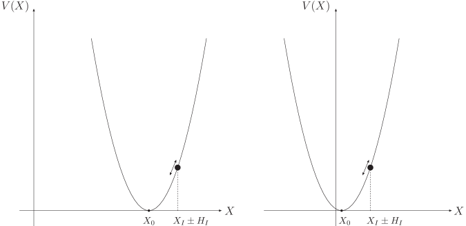
FIG. 1.: Case $X_{0}\gg|X_{I}-X_{0}|\,$ (left panel) vs. $X_{0}\ll|X_{I}-X_{0}|\,$ (right panel).

As discussed in the Introduction, there are however interesting cases in which, due to the evolution of $X$ prior or after $t_{*}\,$, eq. (4) does not apply. The amplitude of modulated perturbations can be easily computed case by case and, although there are several parameters in the model, the final results can be most effectively summarized as a function of the mass and the decay rate of the scalar field $X\,$. The two cases $X_{0}\gg|X_{I}-X_{0}|\,$ and $X_{0}\ll|X_{I}-X_{0}|\,$, see fig. (1), lead to different results, and hence we will consider them separately in the next two subsections.

A Case I: $|X_{I}-X_{0}|\ll X_{0}\leq M_{p}$

Figure (2) summarizes the results for this case. We always demand that $\Gamma_{X}<\Gamma_{*}$, with $\Gamma_{X}$ being the decay rate of $X$, which is a necessary assumption for the generation of modulated perturbations.  We also assume that the $X$-dependent term dominates $\Gamma_{*}$ and $\Gamma_{0}$ can be neglected in eq. (1). For $m_{X}<\Gamma_{*}\,$, the field $X$ is frozen at a value $X_{I}\pm H_{I}\,$ when the modulated perturbations are generated. The assumption $X_{0}<M_{p}$ ensures that its energy density is subdominant at this time.  This will continue to be the case provided $X$ decays sufficiently quickly. The modulated perturbations are then estimated as $\zeta\sim H_{I}/X_{0}\,$. However, if $X$ survives long enough, its energy density can overcome that of the inflaton decay products which, as discussed in the Introduction, redshifts as radiation for $t>t_{*}\,$. While $X$ is initially frozen, as soon as the Hubble parameter drops below $m_{X}\,$, the field starts oscillating about $X_{0}\,$. The amplitude of the oscillations decreases as $a^{-3/2}\,$, where $a$ is the scale factor of the universe, so that the energy density of $X$ redshifts as that of matter. The $X$-dominance occurs when the Hubble parameter is

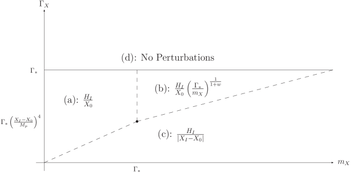
FIG. 2.: The amplitude of perturbations when $X_{0}\gg|X_{I}-X_{0}|\,$. In cases (a) and (b) perturbations are generated before and after the start of $X$ oscillations respectively. Case (c) corresponds to $X$-dominance which is essentially the same as the curvaton scenario. The boundary of (c) with (a) and (b) is defined by $\Gamma_{X}=H_{eq}$, with $H_{eq}$ given in eqs. (5) and (6) respectively.

$$H_{\rm eq}=m_{X}\,\left(\frac{X_{I}-X_{0}}{M_{p}}\right)^{4}\quad\quad\quad,\quad m_{X}<\Gamma_{*}$$ (5)

If $\Gamma_{X}<H_{\rm eq}\,$, the field $X$ dominates before decaying. As a consequence, the relevant primordial perturbations come from fluctuations in the (potential) energy density of $X\,$; $\rho_{X}\propto\left(X_{I}-X_{0}\pm H_{I}\right)^{2}\,$, and hence $\zeta\sim H_{*}/|X_{I}-X_{0}|$ in this case.

If $m_{X}>\Gamma_{*}\,$, the analysis is complicated by the fact that the oscillations of the $X$ field start before $t_{*}\,$. Dominance of $X$ now occurs at

$$H_{\rm eq}=\left(\frac{\Gamma_{*}}{m_{X}}\right)^{\frac{1-3w}{1+w}}\,m_{X}\,\left(\frac{X_{I}-X_{0}}{M_{p}}\right)^{4}\quad\quad\quad,\quad m_{X}>\Gamma_{*}$$ (6)

where $w$ is the (unknown) equation of state of the inflaton decay products for $\Gamma_{*}<H<m_{X}\,$. If the equation of state of the universe changes throughout this interval, the first term on the right-hand side of (6) will be replaced by the product of terms expressing the redshift in each sub-interval. If $\Gamma_{X}<H_{\rm eq}\,$, the $X$ field dominates and perturbations in the energy density of $X$ will give again $\zeta\sim H_{I}/|X_{I}-X_{0}|\,$. For $\Gamma_{X}>H_{\rm eq}\,$, however, modulated perturbations will have a smaller amplitude than the one found above due to the fact that $\delta X$ also decreases as $a^{-3/2}$ during the oscillations of $X\,$.

To summarize, the amplitude of primordial perturbations will amount to

$${H_{I}\over X_{0}}\left({\Gamma_{*}\over m_{X}}\right)^{1\over 1+w}~{}~{}<~{}~{}{H_{I}\over X_{0}}~{}~{}<~{}~{}{H_{I}\over|X_{I}-X_{0}|},$$ (7)

in cases (b), (a) and (c) respectively.  Since $|X_{I}-X_{0}|\ll X_{0}$, obtaining acceptable perturbations requires that $H_{I}/|X_{I}-X_{0}|\geq 10^{-5}$. On the other hand, current limits on the non-gaussianity of perturbations set the upper bound $H_{I}/X_{0}\>\raisebox{-3.22916pt}{$\stackrel{{\scriptstyle\textstyle<}}{{\sim}}$}\>10^{-1}$ [16]. Note that for values close to this limit, perturbations of the correct size can be generated only when $\Gamma_{*}<m_{X}$.

These results should be taken only as estimates of the exact value. More precise values can be obtained once the rate (1) is specified. Clearly, one should not expect a discontinuity of $\zeta$. The amplitude of the adiabatic mode will smoothly interpolate between the values given in fig. (2) and the bordering regions are characterized by a significant amount of isocurvature perturbations.

B Case II: $X_{0}\ll|X_{I}-X_{0}|\leq M_{p}$

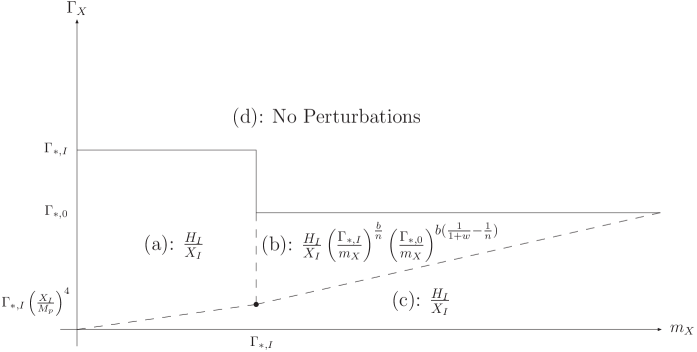
FIG. 3.: The same as fig. (2) but for $X_{0}\ll|X_{I}-X_{0}|\,$. Here $\Gamma_{*,I}$ and $\Gamma_{*,0}$ denote the initial value of $\Gamma_{*}$ and its value in the vacuum respectively. In case (b), domination of $\Gamma_{*,0}$ by $X$-dependent and $X$-independent terms, see eq. (1), results in $b=1$ and $b=n$ respectively.

We now discuss the case where the initial displacement of $X$ is much greater than $X_{0}\,$. In addition, we focus on the situation in which the rate (1) is initially much greater than in the vacuum of the theory, i.e. that $\Gamma_{*,I}\equiv\Gamma_{*}\left(X_{I}\right)\gg\Gamma_{*,0}\equiv\Gamma_{*}\left(X_{0}\right)\,$. Let us first discuss the simpler case $m_{X}<\Gamma_{*,I}\,$, characterized by a frozen field $X$ at $t_{*}\,$. In this case, the analysis is analogous to the one in the previous subsection. If the field $X$ never dominates, the amplitude of modulated perturbations now amounts to $\zeta\sim H_{I}/X_{I}\,$. Remarkably, the same value (up to an ${\cal O}(1)$ factor) is obtained also if the field $X$ survives long enough to dominate, since $\rho\simeq\rho_{X}\propto\left(X_{I}\pm H_{I}\right)^{2}\,$ in this case.

The situation for $m_{X}>\Gamma_{*,I}$ is instead more complicated. As soon as $X$ starts oscillating with a decreasing amplitude, the rate $\Gamma_{*}$ changes according to

$$\Gamma_{*,I}\rightarrow\Gamma\left(X\right)\propto X^{n}\propto H^{\frac{n}{1+w}}\,\,,$$ (8)

where we remind that $w$ denotes the equation of state before $t_{*}\,$. If $n\geq 1+w\,$ (expected, for example, for perturbative processes) $\Gamma_{*}$ decreases more rapidly than (or at the same rate as) $H\,$. Hence, the process which generates modulated perturbations will not be efficient until its rate stabilizes at $\Gamma_{*,0}$. Note that the situation in this case is very different from the one discussed in the previous subsection, where $\Gamma_{*}\simeq\Gamma_{*,0}$ at all times. At $t=t_{*}\,$, the field $X$ evaluates to

$$X\left(t_{*}\right)\simeq\left(X_{I}\pm H_{I}\right)\left(\frac{\Gamma_{*,0}}{m_{X}}\right)^{\frac{1}{1+w}}\,\,.$$ (9)

First assume that $\Gamma_{*,0}\simeq X^{n}_{0}f(X_{0})$, i.e. that the $X$-dependent term dominates in the vacuum. Since $f(X)$ is assumed to be a slowly varying fucntion of $X$, see the discussion after eq. (1), $X_{I}/X_{0}\simeq(\Gamma_{*,I}/\Gamma_{*,0})^{1/n}$ when $n\geq 1+w$. Thus the expression for the ampltiude of perturbations can be cast in the form

$$\zeta\sim{H_{I}\over X_{I}}\left({\Gamma_{*,I}\over m_{X}}\right)^{1/n}\left({\Gamma_{*,0}\over m_{X}}\right)^{{1\over 1+w}-{1\over n}}.$$ (10)

The situation will be somewhat different when the $X$-independent term dominates in the vacuum. Now $\Gamma_{*,0}\simeq\Gamma_{0}$, while $\delta\Gamma_{*,0}\sim X^{n-1}_{I}H_{I}(\Gamma_{*,0}/m_{X})^{n/1+w}$. This results in a smaller value for the amplitude of perturbations

$$\zeta\sim{H_{I}\over X_{I}}\left({\Gamma_{*,I}\over m_{X}}\right)\left({\Gamma_{*,0}\over m_{X}}\right)^{{n\over 1+w}-1}.$$ (11)

If $X$ dominates, we have again $\zeta\sim H_{I}/X_{I}\,$. This occurs provided $X$ decays after $H_{\rm eq}\,$, given by eq. (6).

It turns out from (10) and (11) that $\zeta<H_{I}/X_{I}$ in case (b). It is therefore possible to generate acceptable perturbations in this case for $10^{-5}<H_{I}/X_{I}\>\raisebox{-3.22916pt}{$\stackrel{{\scriptstyle\textstyle<}}{{\sim}}$}\>10^{-1}$. The upper bound is again given by current limits on the non-gaussianity of perturbations. When $H_{I}/X_{I}$ is close to this value, the modulated perturbations mechanism can work even if $X_{I}$ is entirely due to the accumulation of quantum fluctuations, and if inflation does not last much longer than $60$ e-foldings [17]. Note that the last two terms on the right-hand side of (10) and (11) should yield a number $>10^{-4}$. Otherwise oscillations of $X$ will suppress modulated perturbations to an unacceptably low value.

III Particle physics examples of $X$

In this section we present three realistic particle physics examples of $X$. We will discuss different possibilties for generating sufficient perturbations while satisfying other cosmological constraints, particularly to avoid the gravitino problem. As we will point out, these examples actually represent a wide range of particle physics candidates for $X$.

A Moduli

In superstring models physical parameters are usually set by the VEV of moduli scalar fields, which acquire mass only after supersymmetry is broken. In a cosmological setting, supergravity effects typically provide these fields with a mass of the order of the Hubble parameter $H\,$ [18, 19]. However, there are situations in which (for example, due to a “Heisenberg symmetry” [20]) supergravity corrections do not affect some of these directions. These fields may then naturally be expected to have a mass of the order of the low energy supersymmetry breaking; $m_{X}\sim{\cal O}(\rm TeV)$. Moduli are gravitationally coupled to the other fields in the theory, so that their decay rate is estimated to be $\Gamma_{X}\sim m^{3}_{X}/M^{2}_{p}$. They are typically characterized by $X_{0}\sim M_{p}\,$, thus leading to case I in above.

Modulated perturbations can be expected if any parameter relevant for reheating is controlled by one of these fields [7]. However, as we shall see, they turn out to be rather small in this example. The final result for the perturbations is sensitive to the difference $|X_{I}-X_{0}|\,$, namely on the initial displacement of the modulus from the minimum of the potential. We regard this quantity as a free parameter, with the only constraint that it should be greater than the Hubble parameter during inflation $H_{I}$. From eq. (5) we see that for $|X_{I}-X_{0}|\>\raisebox{-3.22916pt}{$\stackrel{{\scriptstyle\textstyle<}}{{\sim}}$}\>10^{11}\,{\rm GeV}\,$ the modulus field decays before it dominates. However, as we just noted, the limit on $|X_{0}-X_{I}|$ povides an upper bound also on $H_{I}$. This results in modulated perturbations that are too small, see fig. (2).

For $|X_{I}-X_{0}|\>\raisebox{-3.22916pt}{$\stackrel{{\scriptstyle\textstyle>}}{{\sim}}$}\>10^{11}$ the modulus decays after it dominates, and the relevant perturbations are the ones in the energy density of $X\,$.  As long as $|X_{I}-X_{0}|<M_{p}\,$, the amplitude of the perturbations amounts to $\sim H_{I}/|X_{I}-X_{0}|\,$ (see fig. 2). Acceptable perturbations are then generated provided $H_{I}\sim 10^{-5}\,|X_{I}-X_{0}|\,$. Actually $m_{X}\>\raisebox{-3.22916pt}{$\stackrel{{\scriptstyle\textstyle>}}{{\sim}}$}\>50$ TeV is needed so that the moduli decay will result in a reheat temperature $\sim{\cal O}(\rm MeV)$, compatible with the big bang nucleosynthesis. This can be achieved while keeping the mass splitting between matter fields and their supersymmetric partners at TeV level, for example, in models of anomaly-mediated supersymmetry breaking [21]. For $|X_{I}-X_{0}|>M_{p}\,$, the modulus $X$ drives a stage of inflation, and the analysis of the previous section does not apply. However, due to the smallness of $m_{X}$,i.e. $m_{X}\ll 10^{13}$ GeV, identification of modulus with the inflaton field results in unacceptably small perturbations.

B Right-handed sneutrinos

The right-handed (RH) sneutrinos arise in supersymmetric extensions of the standard model [22] which explain the smallness of the mass of the left-handed (LH) neutrinos via the see-saw mechanism [23]. A non-zero VEV for ${\tilde{N}}$ at the minimum of its potential breaks $R$-parity, thus destabilizing the lightest supersymmetric particle (LSP) [22]. This VEV should be $\ll 1$ GeV, if the LSP survives until today and constitutes the dark matter. Nevertheless, since $\tilde{N}$ is a standard model gauge singlet, it is conceivable that the $X$-indepdendent contribution to the process which generates modulated perturbations can be recasted in a much larger $X_{0}\,$, as we have discussed after eq. (3). Consider an example where perturbations are imprinted at the inflaton decay which proceeds through the superpotential couplings (the boldface charachters denote superfields)

$${{\bf X}\over M_{p}}\Phi\Psi\Psi+h\Phi\Psi\Psi.$$ (12)

Then $X_{0}=hM_{p}$, leading to case I (II) in above if $X_{I}\ll hM_{p}$ ($\gg hM_{p}$). We concentrate on the latter possibility as the former will lead to a situation similar to that discussed in the previous subsection. 

The see-saw formula gives [23]

$$m_{X}\geq y^{2}\langle H\rangle^{2}/m_{\nu}\sim y^{2}\,10^{15}\,{\rm GeV}\,\,,$$ (13)

where $\langle H\rangle\sim 200$ GeV is the electroweak symmetry breaking scale, $m_{\nu}\simeq 0.05$ eV is the mass of the heaviest light neutrino and $y$ denotes the neutrino Yukawa coupling. The same interactions give rise to a sneutrino decay rate

$$\Gamma_{X}=\frac{y^{2}}{8\,\pi}m_{X}\sim y^{4}\,10^{14}\,{\rm GeV}\,\,.$$ (14)

In realistic models of neutrino masses based on the see-saw mechansim [24], $m_{X}$ is typically much larger than the scale of electroweak symmetry breaking. Moreover, producing sufficient baryon asymmetry via leptogenesis [25] leads to additional constraints on the model parametrs. In particular, various leptogenesis scenarios [26, 27, 28, 29, 30] require that $m_{X}>10^{5}$ GeV (for thermal leptogenesis the bound is about $4$ order of magnitude stronger) unless some specific fine-tuning occurs (for example, having nearly degenerate RH (s)neutrinos [31]). Therefore, $m_{X}\gg 1$ TeV in general.

In principle, $\Gamma_{*}$ can be larger or smaller than $m_{X}\,$. In the former case, modulated perturbations must be generated by a very rapid process, most notably non-perturbative inflaton decay via preheating. A large $\Gamma_{*}\,$ may be associated with a high reheat temperature $T_{R}\,$,  which can then lead to thermal overproduction of gravitinos. In gravity-mediated models of supersymmetry breaking the gravitino mass is $m_{3/2}\simeq 100~{}{\rm GeV}-1$ TeV and (up to logarithmic factors) [33]

$${n_{3/2}\over s}\simeq 10^{-12}\left({T_{R}\over 10^{9}~{}{\rm GeV}}\right).$$ (15)

Bounds from nucleosynthesis (due to photodissociation of light elements by gravitino decay products) impose $T_{R}\leq 10^{9}$ GeV [34], corresponding to $H_{R}\leq 10$ GeV ($H_{R}$ being the Hubble parameter at $T=T_{R}$). In models of gauge-mediated supersymmetry breaking, the gravitino is the LSP and $m_{3/2}$ can be as low as $1$ KeV. Its fractional energy density is in this case [35, 36]

$$\Omega_{3/2}h^{2}\simeq 0.8\left({M_{3}\over 1~{}{\rm TeV}}\right)^{2}\left({10~{}{\rm MeV}\over m_{3/2}}\right)\left({T_{R}\over 10^{6}~{}{\rm GeV}}\right),$$ (16)

where $h\approx 0.7$ and $M_{3}$ is the gluino mass parameter. Then, for a typical value $M_{3}\sim 500$ GeV, the dark matter limit results in $T_{R}\>\raisebox{-3.22916pt}{$\stackrel{{\scriptstyle\textstyle<}}{{\sim}}$}\>10^{8}\,m_{3/2}$, corresponding to $H_{R}\leq 10^{17}m^{2}_{3/2}/M_{p}$. In both cases higher $T_{R}$ can be accommodated, provided the gravitino abundance is diluted by an entropy release at later times. This entropy can be naturally provided by the decay of the sneutrino if its energy density becomes significantly greater than that of the thermal bath. In addition, the observed baryon asymmetry of the universe can also be generated by such a late decay [29, 30]. Then (5), (14), (15) and (16) lead to the bounds

$$y\leq 5\left({10^{9}~{}{\rm GeV}\over T_{R}}\right)\left({X_{I}-X_{0}\over M_{p}}\right)^{2},$$ (17)

and

$$y\leq 5\times 10^{8}\left({m_{3/2}\over T_{R}}\right)\left({X_{I}-X_{0}\over M_{p}}\right)^{2}$$ (18)

in gravity-mediated and gauge-mediated models respectively. We are thus naturally led to consider the case in which the sneutrino dominates. Primordial perturbations will then be related to fluctuations in the energy density of $X\,$, corresponding to case (c) in fig. (3).

Let us finally consider the case where $\Gamma_{*,I}<m_{X}\,$. If the reheat temperature respects the gravitino bound, no entropy generation will be required. Then the sneutrino may decay before or after dominating the universe corresponding to cases (b) and (c) in fig. (3), respectively, and perturbations will be given by (10) in the former case. If the reheat temperature exceeds the gravitino bound, sneutrino dominance will be favoured again to solve the gravitino problem.

C Supersymmetric flat directions

There are many directions in the space of the Higgs, slepton and squark fields along which the scalar potential of the MSSM identically vanishes in the limit of exact supersymmetry [37]. These flat directions acquire a mass from supersymmetry breaking. In gravity-mediated models $m_{X}=100~{}{\rm GeV}-1$ TeV [22]. In gauge-mediated models $m_{X}\simeq 100~{}{\rm GeV}-1$ TeV for small $\langle X\rangle$, it drops $\propto\langle X\rangle^{-1}$ at intermediate VEVs and $m_{X}\sim m_{3/2}$ for large $\langle X\rangle$ [36].

The Higgs fields have a VEV $\sim 100$ GeV in the vacuum, while those of the sleptons and squarks vansih. Therefore identification of $X$ with the MSSM flat directions (the primary example considered in [6]) leads to case II in above where perturbations read from fig. (3). The situation is qualitatively similar to the sneutrino example but some differences exist. For the flat directions $m_{X}$ is typically much smaller than the RH sneutrinos, particularly in gauge-mediated models. This allows a smaller $\Gamma_{*}$ (as expected for perturbative processes) when $\Gamma_{*,I}>m_{X}$. The fact that the Higgs, slepton and squark fields are gauge non-singlets can also result in a different situation when $\Gamma_{*,I}<m_{X}$. Consider again the example of inflaton decay in eq. (12), with $X$ being a Higgs, slepton or squark field. Now the two terms in (12) must couple the inflaton to different final states $\Psi_{1}$ and $\Psi_{2}$, resulting in decay rates $\Gamma_{X}$ and $\Gamma_{0}$ respectively. In any acceptable scenario $\Gamma_{*,0}\simeq\Gamma_{0}$, and hence perturbations will be given by (11), instead of (10) for the sneutrinos, provided $X$ does not dominate.

The $X$-dominance leads to case (c) in fig. (3). The decay of the flat directions proceeds through the SM Yukawa and gauge couplings. In particular, one may wonder whether $X$ can dominate at all as gauge couplings lead to a rapid decay of $X$. However, the gauge (and Yukawa) couplings also result in an effective mass $m_{eff}$ for the decay prodcuts due to their couplings to the $X$ condensate and thermal effects. The decay is kinematically forbidden so long as $m_{eff}>m_{X}$ [39]. It occurs when $H=H_{d}\equiv{\rm min}[\Gamma_{X},H_{kin}]$, with $H_{kin}$ denoting the value of Hubble parameter at which $m_{eff}$ drops below $m_{X}$.  Therefore $X$-dominance actually requires that $H_{d}<H_{eq}$, where $H_{eq}$ is given by (6).

D Summary

In supergravity models all scalar fields typically receive a supersymmetry breaking mass $\sim m_{3/2}$. If a supersymmetry conserving (superpotential) mass term is allowed for a field, its mass can be $\gg m_{3/2}$. However, a tree-level (supersymmetry breaking or conserving) mass term will be forbidden if the theory has some symmetry in the superpotential (thus resulting in a Goldstone boson) or in the kinetic function (as in no-scale supergravity [40]). In this case the corresponding field obtains a mass $\ll m_{3/2}$ through symmetry breaking interactions at higher orders. Thus, unless forbidden by some symmetry, $m_{X}\geq m_{3/2}$ will be expected in general. Under the most general circumstances, a massive scalar field is either in a hidden sector, thus gravitationally coupled to the SM fields, or has gauge and/or Yukawa couplings to the observable sector. Moduli are an example of the case with $m_{X}\sim m_{3/2}$ and gravitational decay to matter fields. The supersymmetric flat directions ($m_{X}\geq m_{3/2}$) and the RH sneutrinos ($m_{X}\gg m+{3/2}$) have gauge and Yukawa couplings to the SM fields. The three examples considered above therefore represent a wide range of possible $X$ candidates.

One comment is in order before closing this section. We have only considered the mass term in $V(X)$, see (3). However, higher order terms are naturally expected to arise and make the potential steeper than $X^{2}$ at large field values. This will result in an upper limit $X_{max}$ on $X_{I}$ at which $V^{\prime\prime}(X_{max})\sim H^{2}_{I}$. When $X_{I}\simeq X_{max}$, fluctuations of $X$ are attenuated even before oscillations start [41]. This will suppress the amplitude of perturbations compared to that is given in figs. (2) and (3), which will be valid so long as $X_{I}<X_{max}$. A limit on $X_{I}$, through the expressions for the amplitude of perturbations, translates into an upper bound on the scale of inflation $H_{I}$. The strongest bound $H_{I}<10^{-5}X_{max}$ is obtained when $\zeta\sim H_{I}/X_{I}$, while cases with $\zeta<H_{I}/X_{I}$ lead to weaker constraints on $H_{I}$. In particular, $H_{I}$ can be just one order of magnitude below $X_{max}$ when the value of $H_{I}/X_{I}$ is close to the current limit from non-gaussianity of perturbations. The bound on $H_{I}$ can in this case be comparable with (or weaker than) $H_{I}<10^{13}$ GeV, which is required so that the inflaton fluctuations not yield too large perturbations, even if $X_{max}\ll M_{p}$. The value of $X_{max}$, signifying the importance of higher order terms, strongly depends on the particle physics identification of $X$. For a modulus field these terms are $M_{p}$ suppressed and the mass term will be dominant up to $X_{I}\>\raisebox{-3.22916pt}{$\stackrel{{\scriptstyle\textstyle<}}{{\sim}}$}\>M_{p}$ . For the RH sneutrinos and supersymmetric flat directions, $X_{max}$ can assume a wide range of values $\ll M_{p}$. Due to the model-dependence of $X_{max}$ and the constraint it imposes on $H_{I}$, we have not considered higher order terms in $V(X)$ in our discussion.

IV Discussion

So far we have assumed that only the inflaton and the $X$ field dynamically evolve in the early universe. Any other scalar fields with masses smaller than $H_{I}$ are also expected to acquire inflationary fluctuations, and be substantially displaced from the minimum of their potential at early times. They can then contribute to density perturbations in a similar fashion as the $X$ field. Since $X$ is considered to be the dominant source for generating perturbations here, fluctuations of other scalar fields should be suppressed. This is particularly true for $X$ decay products, generally denoted by $\chi$. This can be naturally achieved if these fields have a mass $\>\raisebox{-3.22916pt}{$\stackrel{{\scriptstyle\textstyle>}}{{\sim}}$}\>H_{I}$ during inflation. One possibility is that supergravity effects provide such a mass [18, 19]. Note, however, that the supergravity mass for $X$ should be $<H_{I}$. As pointed out earlier, this can happen if $X$ has a different kinetic function from other fields. It is also possible that different masses for different fields arise dynamically as a result of quantum corrections [42, 43]. Fluctuations of $\chi$ will also be suppressed if its coupling to $X$ and/or inflaton, denoted by $y$ and $h$ respectively, is sufficiently large, i.e. that $yX_{I}>H_{I}$ and $h\phi_{0}>H_{I}$ respectively ($\phi_{0}$ is the initial amplitude of inflaton oscillations). Since $m_{X}<H_{I}$, preheating decay of $X$ and/or inflaton to $\chi$ will be expected in this case [4].

The discussion of Section III, together with the requirement for suppressing fluctuations of $\chi$, lead us to the following “benchmark scenarios” for modulated perturbations:

1. $X$ is in the hidden sector and $m_{X}\>\raisebox{-3.22916pt}{$\stackrel{{\scriptstyle\textstyle>}}{{\sim}}$}\>50$ TeV. Supergravity effects provide a mass $>H$ for $\chi$ suppressing its fluctuations. $X$ dominates the universe and fluctuations in its energy density give rise to perturbations; case (c) in fig. (2). The situation is essentially the same as the curvaton scenario.

2. $X$ is in the observable sector and $m_{X}\gg 1$ TeV. Perturbations are generated when the inflaton decyas via preheating, before $X$ starts oscillating; case (a) in fig. (3). Coupling of $X$ to $\chi$ is large enough ($y>10^{-5}$) to suppress its fluctuations. This also leads to a rapid non-perturbative decay of $X$ to $\chi$, which is welcome as $X$ will not dominate and consequently affect perturbations. The universe thermalizes sufficiently late, thus there will be no thermal overproduction of gravitinos and no late time entropy generation will be required.

3. $X$ is in the observable sector and starts oscillating before perturbations are imprinted; case (b) in fig. (3). This happens due to the slowness of the process generating perturbations, for example, gravitational decay of the inflaton or decay of a long-lived massive particle produced in the inflaton decay. Such a slow process will be required by the gravitino bound when the universe thermalizes rapidly. Oscillations of $X$ in this case suppress modulated perturbations compared to that in the previous scenario. Preheating decay of $X$ is not allowed, thus $yX_{I}<m_{X}$, since it should survive long enough until perturbations are generated. This rules out suppressing $\chi$ fluctuations through its coupling to $X$ (supergravity effects or a large coupling to the inflaton can do this instead). On the other hand, since fluctuations in the energy density of $X$ can be $\gg 10^{-5}$, $X$ must decay long before dominating in order not to affect perturbations. This, after using (6), will result in an upper bound on $y$.

   We note that $X$ can undergo early oscillating if it acquires a large thermal [44] or non-thermal [45] mass $m_{X,eff}$. This will happen provided $\chi$ are in equilibrium with the (p)reheat plasma and $y$ is sufficiently large,  so that $m_{X,eff}$ exceeds the Hubble parameter when $H>m_{X}$.

4. $X$ is in the observable sector and starts oscillating before or after modulated perurbations are generated. The reheat temperature exceeds the gravitino bound but $X$ dominates the universe before decaying, thus diluting the gravitinos in excess. Fluctuations of $\chi$ will in this case be suppressed by supergravity effects or a large coupling to the inflaton. Perturbations will be due to fluctuations in the energy density of $X$; case (c) in fig. (3).

V Summary and conclusions

In this paper we have studied different scenarios of modulated perturbations. In this mechanism adiabatic cosmological perturbations are generated during reheating when the equation of state in the different parts of the universe changes at different moments. The inhomogeneity arises due to inflationary fluctuations of some scalar field $X$ whose VEV controls the value of parameter(s) (such as mass or coupling) involved in the relevant process. This is a generic property expected in models based on superstring and supersymmetric theories. Depending on the values of the rate of the process $\Gamma_{*}$, mass of the scalar field $m_{X}$ and its decay rate $\Gamma_{X}$, different situations can arise. We presented a general analysis of possible scenarios, with the main results summarized in fig. (2) and fig. (3). We also introduced some specific particle physics examples including the string moduli, RH sneutrinos and supersymmetric flat directions. These examples, in which $m_{X}$ is of the same order or greater than the gravitino mass $m_{3/2}$, represent a wide range of particle physics candidates of $X$.

The simplest possibility is that perturbations are generated when $X$ is frozen at an initial value $X_{I}$. If $m_{X}\geq{\cal O}(\rm TeV)$ (as for the RH sneutrinos and supersymmetric flat directions), this requires a very rapid process, namely non-perturbative inflaton decay via preheating. Moreover, $X$ must decay before dominating the energy density of the universe, and the reheat temperature should be sufficiently low to avoid overproduction of gravitinos. For a slower (likely perturbative) process, $X$ can start oscillating around the minimum of its potential before perturbations are imprinted. Then the expansion of the universe redshifts fluctuations of $X$ and dampens perturbations. An interesting consequence is that the level of non-gaussianity can in this case be just below the current limits and accessible to future experiments. If $X$ is long-lived (for example, a modulus field), it can dominate the universe before decaying. In this case the situation will essentially be the same as the curvaton scenario and fluctuations in the energy density of $X$ give rise to perturbations. The $X$-dominance can be a virtue when the reheat temperature exceeds the gravitino bound necessitating late time entropy production. The amplitude of the adiabatic mode is in general very different from one case to another. It interpolates between the different values and bordering regions are charachterized by a significant isocurvature component.

In conclusion, the modulated perturbations mechanism is a viable alternative with potentially interesting observational consequences. It can be implemented in various ways and a successful particle physics identification can lead us to a clearer and more complete picture of reheating.

VI Acknowledgements

The author wishes to thank L. Kofman and M. Peloso for many valuable discussions and collaboration at earlier stages of this work, and R. Cyburt for careful reading of the manuscript. He also acknowledges the kind hospitality by CITA while this work was being completed. The research of R.A. is supported by the National Sciences and Engineering Research Council of Canada.

REFERENCES

-
[1]
For reviews on inflation, see: A. D. Linde, Particle Physics and
Inflationary Cosmology, Harwood (1990);
D. H. Lyth and A. Riotto, Phys. Rep. 314, 1 (1999). - [2] C. L. Bennett, et al, Ap. J. S. 148, 1 (2003); D. N. Spergel, et al, Ap. J. S. 148, 175 (2003).
- [3] A. Dolgov and A. D. Linde, Phys. Lett. B 116, 329 (1982); L. F. Abbott, E. Farhi and M. Wise, Phys. Lett. B 117, 29 (1982).
- [4] L. Kofman, A. D. Linde and A. A. Starobinsky, Phys. Rev. Lett. 73, 3195 (1994), and Phys. Rev. D 56, 3258 (1997).
- [5] G. Lazarides and Q. Shafi, Phys. Lett. B 258, 305 (1991); E. W. Kolb, A. D. Linde and A. Riotto, Phys. Rev. Lett. 77, 4290 (1996).
- [6] G. Dvali, A. Gruzinov and M. Zaldarriaga, Phys. Rev. D 69, 023505, (2004); ibid 69, 083505 (2004).
- [7] L. Kofman, astro-ph/0303614.
- [8] M. Postma, J. Cosmol. Astropart. Phys. 0403, 006 (2004).
- [9] A. Gruzinov, astro-ph/0401407.
- [10] D. H. Lyth and D. Wands, Phys. Lett. B 524, 5 (2002); D. H. Lyth, C. Ungarelli and D. Wands, Phys. Rev. D 67, 023503 (2003).
- [11] T. Moroi and T. Takahashi, Phys. Lett. B 522, 215 (2001), Erratum-ibid B 539, 303 (2002); Phys. Rev. D 66, 063501 (2002).
- [12] N. Bartolo and A. R. Liddle, Phys. Rev. D 65, 121301 (2002).
- [13] K. Dimopoulos, G. Lazarides, D. H. Lyth and R. Ruiz de Austri, Phys. Rev. D 68, 123515 (2003).
- [14] P. Greene and L. Kofman, Phys. Lett. B 448, 6 (1999), and Phys. Rev. D 62, 123516 (2000).
- [15] M. Peloso and L. Sorbo, J. High Energy Phys 0005, 016 (2000).
- [16] E. Komatsu, D. N. Spergel and B. D. Wandelt, astro-ph/0305189.
- [17] G. Felder, L. Kofman and A. D. Linde, J. High Energy Phys. 0002, 027 (2000).
- [18] M. Dine, W. Fischler and D. Nemechansky, Phys. Lett. B 138, 169 (1984); S. Bertolami and G. G. Ross, Phys. Lett. B 183, 163 (1987); G. Dvali, Phys. Lett. B 355, 78 (1995).
- [19] M. Dine, L. Randall and S. Thomas, Phys. Rev. Lett. 75, 398 (1995), and Nucl. Phys. B 458, 291 (1996).
- [20] P. Binetruy and M. K. Gaillard, Phys. lett. B 195, 382 (1987).
- [21] G. F. Giudice, M. A. Luty, H. Murayama and R. Rattazzi, J. High Energy Phys. 9812, 027 (1998).
- [22] For a review on supersymmetry, see: H. P. Nilles, Phys. Rept. 110, 1 (1984).
- [23] M. Gell-Mann, P. Ramond and R. Slansky, in Supergravity, eds. P. van Nieuwenhuizen and D. Z. Freedman (North Holland 1979); T. Yanagida, Proceedings of Workshop on Unified Theory and Baryon number in the Universe, eds. O. Sawada and A. Sugamoto (KEK 1979); R. N. Mohapatra and G. Senjanovic, Phys. Rev. Lett. 44, 912 (1980).
- [24] For a review on neutrino mass models, see: S. F. King, Rept. Prog. Phys. 67, 107 (2004), and references therein.
- [25] M. Fukugita and T. Yanagida, Phys. Lett. B 174, 45 (1986).
- [26] W. Büchmuller, P. Di bari and M. Plümacher, Nucl. Phys. B 643, 367 (2002); Nucl. Phys. 665, 445 (2003), and hep-ph/0401240.
- [27] S. Davidson, J. High Energy Phys. 0303, 037 (2003).
- [28] G. F. Giudice, A. Notari, M. Raidal, A. Riotto and A. Strumia, Nucl. Phys. B 685, 89 (2004).
- [29] K. Hamaguchi, H. Murayama and T. Yanagida, Phys. Rev. D 65, 043512 (2002).
- [30] R. Allahverdi and M. Drees, Phys. Rev. D 69, 103522 (2004).
- [31] A. Pilaftsis, Phys. Rev. D 56, 5431 (1997), and Int. J. Mod. Phys. A 14, 1811 (1999); A. Pilaftsis and T. E. J. Underwood, hep-ph/0309342.
- [32] A. Mazumdar, Phys. Lett. B 580, 7 (2004), and Phys. Rev. Lett. 92, 241301 (2004).
-
[33]
M. Yu. Khlopov and A. D. Linde, Phys. Lett. B 138, 265 (1984);
J. Ellis, J. E. Kim and D. V. Nanopoulos, Phys. Lett. B 145,
181 (1984);
J. Ellis, D. V. Nanopoulos, K. A. Olive and S- J. Rey, Astropart. Phys.
4, 371 (1996);
for a recent calculation, see: M. Boltz, A. Brandenburg and W. Büchmuller, Nucl. Phys. B 606, 518 (2001). -
[34]
R. H. Cyburt, J. Ellis, B. D. Fields and K. A. Olive, Phys. Rev. D 67,
103521 (2003).
for a review, see: S. Sarkar, Rept. Prog. Phys. 59, 1493 (1996). - [35] T. Moroi, H. Murayama and M. Yamaguchi, Phys. Lett. B 303, 289 (1993).
- [36] A. de Gouvêa, T. Moroi and H. Murayama, Phys. Rev. D 56, 1281 (1997).
-
[37]
T. Gherghetta, C. Kolda and S. Martin, Nucl. Phys. B 468, 37 (1996):
for a review on cosmological consequences of flat directions, see: K. Enqvist and A. Mazumdar, Phys. Rep. 380, 99 (2003). - [38] A. Kusenko and M. Shaposhnikov, Phys. Lett. B 418 (1998) 46; K. Enqvist and J. McDonald, Phys. Lett. B 425 (1998) 309.
- [39] A. D. Linde, Phys. Lett. B 160, 243 (1985).
- [40] E. Cremmer, S. Ferrara, C. Kounnas and D. V. Nanopoulos, Phys. Lett. B 133, 61 (1983).
- [41] K. Enqvist, A. Mazumdar and M. Postma, Phys. Rev. D 67, 121303 (2003).
- [42] M. K. Gaillard, H. Murayama and K. A. Olive, Phys. Lett. B 355, 71 (1995).
- [43] R. Allahverdi, M. Drees and A. Mazumdar, Phys. Rev. D 65, 065010 (2002).
- [44] R. Allahverdi, B. A. Campbell and J. Ellis, Nucl. Phys. B 579, 355 (2000); A. Anisimov and M. Dine, Nucl. Phys. B 619, 729 (2001).
- [45] L. Kofman, A. D. Linde and A. A. Starobinsky, Phys. Rev. Lett. 76, 1011 (1996); I. I. Tkachev, Phys. Lett. B 376, 35 (1996).