Origin of coherent magnetic fields in high redshift objects

Abstract

Large scale strong magnetic fields in galaxies are generally thought to have been generated by a mean field dynamo. In order to have generated the fields observed, the dynamo would have had to have operated for a sufficiently long period of time. However, magnetic fields of similar intensities and scales to the one in our galaxy, are observed in high redshift galaxies, where a mean field dynamo would not have had time to produce the observed fields. Instead of a mean field dynamo, we study the emergence of strong large scale magnetic fields in the first objects formed in the universe due to the action of a turbulent, helical stochastic dynamo, for redshifts $5\leq z\leq 10$. Ambipolar drift plays an important role in this process due to the low level of ionization of the gas, allowing a large scale stochastic dynamo to operate. We take into account the uncertainties in the physics of high redshift objects by examining a range of values for the parameters that characterize the turbulent plasma. By numerically integrating the nonlinear evolution equations for magnetic field correlations, we show that for reasonable values of the parameters in the time interval considered, fields can grow to high intensities ($\sim 10^{-6}$ G), with large coherence lengths ($\sim 2-6$ kpc), essentially independent of the initial values of the magnetic field.

1 INTRODUCTION

Magnetic fields have been observed in all known structures of our universe, from the Earth to superclusters of galaxies, spanning a wide range of intensities from $\sim\mu\,\rm{G}$ in galaxies and galaxy clusters to $\sim 10^{\,12}\,\rm{G}$ in neutron stars. The origin of these fields in large structures, such as galaxies and clusters of galaxies, remains an unsolved problem. Many physical processes have been proposed to explain the origin and evolution of these fields (see reviews Grasso & Rubinstein, 2001; Widrow, 2002). The processes suggested can be divided into two main classes: 1) cosmological mechanisms; and 2) local astrophysical processes. Until now, none of them has provided a satisfactory explanation for the generation of the magnetic fields.

A mean field dynamo is commonly invoked to explain the fields observed in our galaxy and in small redshift galaxies (e.g., Zel’dovich et al., 1983; Moffat, 1978). In order to have attained the observed intensities, the dynamo would have had to have operated for a time on the order of the age of the universe. However, the presence of equally intense and coherent fields in high redshift galaxies (Carrilli & Taylor, 2002), where the mean field dynamo would not have had enough time to amplify the field to the observed values, casts doubt on the mean field dynamo paradigm as the preferred generation mechanism. Fields of similar intensity and coherence to those in the Milky Way, have also been detected in high redshift damped $\rm{Lyman}-\alpha$ systems (Wolfe et al., 1992).

In this paper, we are concerned with the origin of strong, large coherent magnetic fields in high redshift structures. We relate the origin of magnetic fields to the physical conditions in the early universe: 1) a dense low ionized plasma; and 2) appreciable turbulence due to the observed high star formation rate (Lanzetta et al. lanzetta02, 2002).

The formation of the first stars and quasars marked the beginning of the transformation of the universe from a smooth initial state to its present lumpy state. In the bottom-up hierarchy of cold dark matter (CDM) cosmologies, the first gaseous clouds collapsed at redshifts $z>10$ and, subsequently, fragmented into stars due to molecular hydrogen cooling (Barkana & Loeb, 2001). These collapsing objects then fragmented into many clumps, which had typical masses of $\sim 10^{\,2}-10^{\,3}M_{\odot}$. Very massive stars have lifetimes of $\sim 3\times 10^{\,6}\,\rm{years}$ and end their lives as supernovae.

Recently, Lanzetta et al. (lanzetta02, 2002) showed that the incidence of the highest intensity star formation regions increases monotonically with redshift. Their observations indicate that star formation in the early universe occurred at a much higher rate than was previously believed. Therefore, the rate of occurrence of supernovae would have also been much higher in the past than at the present. Supernovae shocks disturb the plasma in which they are immersed, producing turbulent motions of the gas. If the supernovae rate was much higher in the past than at present, the plasma of the first formed objects must have been much more turbulent than that of presently observed, low redshift, star forming galactic molecular clouds.

Turbulence generates stochastic magnetic fields (magnetic noise) at a faster rate than it does mean fields (Kulsrud & Anderson, 1992). If the turbulence is strongly non-helical, the fields induced are confined to small scales (Kazantzev kazantzev68, 1968). However, if it is helical, induction of large scale magnetic correlations by the $\alpha$ effect occurs (Vainshtein & Kichatinov vainshtein86, 1986). Astrophysical turbulence is mainly of a helical nature. Hence, we can expect that large scale correlations were induced by the high redshift, turbulent plasma.

In this study, we explore the hypothesis that the magnetic fields observed in high redshift galaxies were created by small scale, stochastic, turbulent helical dynamos, rather than by mean field dynamos. We use a simple model of a gas cloud that is assumed to have collapsed at a high redshift $z>10.$ At $z\sim 10,$ the cloud would have had a low magnetization level and a high level of turbulence. Thus, it would have been similar to the turbulent, low ionization, star forming molecular clouds observed in our galaxy, albeit with a much smaller initial magnetic field and a much higher turbulence level due to the higher star formation rate in the early universe.

It is well known that shock waves produced by supernova explosions accelerate cosmic rays to energies $\geq\,\rm{GeV}$ (e.g., Blandford & Eichler, 1987). Völk et al. (volk89, 1989) showed that in all galaxies, the supernova rate is a direct measure of the cosmic ray intensity. We can, therefore, infer that cosmic rays were already present in considerable intensities in high redshift galaxies. We take into account phenomenologically, the effect on turbulence of cosmic rays, supernova shocks, and powerful stellar winds from massive stars on turbulence by varying the turbulent parameters over a broad range, in order to take into account the uncertainies in our knowledge of high redshift structures.

The linear evolution equations for the correlation function of magnetic fields for non-helical turbulence were derived nearly forty years ago by Kazantzev (kazantzev68, 1968). For helical turbulence, the corresponding equations were obtained twenty years later by Vainshtein & Kichatinov (vainshtein86, 1986). These equations are linear in the magnetic correlations. Recently, Subramanian (subramanian99, 1999) and Brandemburg & Subramanian (bran-sub, 2000) derived the non-linear evolution equations for the magnetic correlations by taking into account the back-reaction of the Lorentz force on the plasma charges in the form of ambipolar drift. We solve the nonlinear helical evolution equations numerically for various values of the parameters that characterize the high redshift turbulent plasma.

The paper is organized as follows. In section II, we give the evolution equations for the magnetic correlations. We describe the effects of the main parameters on the integration in section III . Finally, in section IV, we summarize and discuss our results.

2 MAGNETIC FIELD EVOLUTION EQUATIONS

In this section, we summarize the nonlinear evolution equations for the magnetic field correlations (Subramanian subramanian99, 1999, Brandemburg & Subramanian bran-sub, 2000). The evolution equation for the magnetic field is given by the induction equation, $\partial\,\mathbf{B}/\partial\,t=\mathbf{\nabla\times}\left(\mathbf{v\times{B}}-\eta\mathbf{\nabla\times\mathbf{B}}\right),$ where $\mathbf{B}$ is the magnetic field, $\mathbf{v}$ the velocity of the fluid, and $\eta$ is the Ohmic resistivity. The velocity $\mathbf{v}$ $(=\mathbf{v}_{\,T}+\mathbf{v}_{D})$ is the sum of an external stochastic field $\mathbf{v}_{\,T}$ and an ambipolar drift component $\mathbf{v}_{D},$ which describes the non-linear back-reaction of the Lorentz force. This back-reaction is due to the force that the ionized gas exerts on the neutral gas through collisions of the ions with the neutral atoms. It is assumed that $\mathbf{v}_{\,T}$ is an isotropic, homogeneous, Gaussian random field with a zero mean value and a delta correlation function in time (Markovian approximation). Its two point correlation function is $\left\langle{v_{\,T}^{\,i}\left(\mathbf{x},t\right)v_{\,T}^{\,j}\left(\mathbf{y},s\right)}\right\rangle=T^{\,ij}(\mathbf{r})\delta(t-s),$ where $T^{\,ij}\left(\mathbf{r}\right)=T_{NN}\left(\mathbf{r}\right)\left[\,\delta^{\,ij}-{r^{\,i}r^{\,j}}/{r^{\,2}}\,\right]+T_{LL}\left(\mathbf{r}\right)\left({r^{\,i}r^{\,j}}/{r^{\,2}}\right)+C\left(\mathbf{r}\right)\epsilon^{\,ijf}r_{f}$ (Monin & Yaglom, 1975). The symbol $\left\langle{}\right\rangle$ denotes ensemble averaging over the stochastic velocities, $r=\left|\mathbf{x}-\mathbf{y}\right|,$ $r^{\,i}=x^{\,i}-y^{\,i},$ $T_{LL}\left(r\right)$ and $T_{NN}\left(r\right)$ are the longitudinal and transverse correlation functions of the velocity field, respectively, and $C\left(r\right)$ is the helical term of the velocity correlations. As the magnetic field grows, the Lorentz force acts on the fluid. We assume that the fluid responds instantaneously and develops an extra drift velocity, proportional to the instantaneous Lorentz force. We, thus, express the drift velocity as $\mathbf{v}_{D}=a\left[\left(\mathbf{\nabla\times B}\right)\times\mathbf{B}\right],$ where $a=\tau/4\pi\rho_{\,i}$, $\tau$ the characteristic response time, and $\rho_{\,i}$ is the ion density.

Consider a system whose size $S\gg L_{c},$ where $L_{c}$ is the coherence scale of the turbulence, for which the mean field averaged over any scale is negligible. We take $\mathbf{B}$ to be a homogeneous, isotropic, Gaussian random field with a negligible mean average value. Thus, we take the equal time, two point correlation of the magnetic field as

$$\left\langle B^{\,i}\left(\mathbf{x},t\right)B^{\,j}\left(\mathbf{y},t\right)\right\rangle=M^{\,ij}\left(r,t\right),$$ (1)

where

$$M^{\,ij}=M_{N}\left[\delta^{\,ij}-\left(\frac{r^{\,i}r^{\,j}}{r^{\,2}}\right)\right]+M_{L}\left(\frac{r^{\,i}r^{\,j}}{r^{\,2}}\right)+H\epsilon_{\,ijk}\,r^{\,k}$$ (2)

(Subramanian subramanian99, 1999). The symbol $\left\langle{}\right\rangle$ denotes a double ensemble average over both the stochastic velocity and $\mathbf{B}$ fields, $M_{L}\left(r,t\right)$ and $M_{N}\left(r,t\right)$ are the longitudinal and transverse correlation functions, respectively, of the magnetic field, and $H\left(r,t\right)$ is the helical term of the correlations. Graphically, $M_{L}$ can be represented as $\rightarrow--\rightarrow$ and $M_{N},$ as $\uparrow--\uparrow.$ Hence, positive values of $M_{L}$ and $M_{N}$ correspond to parallel vectors and negative values, to anti-parallel vectors. Since $\mathbf{\nabla\cdot{B}}=0,$ we have $M_{N}=\left(1/2\,r\right)\partial\left(r^{\,2}M_{L}\right)/\left(\partial r\right)$ Monin & Yaglom (1975). The induction equation can be converted into evolution equations for $M_{L}$ and $H:$

$$\frac{\partial M_{L}}{\partial\,t}\left(r,t\right) = \frac{2}{r^{\,4}}\frac{\partial}{\partial\,r}\left(r^{4}\kappa_{N}\left(r,t\right)\frac{\partial M_{L}\left(r,t\right)}{\partial\,r}\right)$$ (3)

$$+ G(r)M_{L}\left(r,t\right)+4\,\alpha_{N}H\left(r,t\right),$$

$$\frac{\partial H}{\partial{\,t}}\left(r,t\right) = \frac{1}{r^{\,4}}\frac{\partial}{\partial{\,r}}\left[r^{\,4}\frac{\partial}{\partial{\,r}}\left[\,2\,\kappa_{N}\left(r,t\right)H\left(r,t\right)\right.\right.$$ (4)

$$- \left.\left.\alpha_{N}\left(r,t\right)M_{L}\left(r,t\right)\right]\,\right],$$

where

$$\kappa_{N}\left(r,t\right)=\eta+T_{LL}\left(0\right)-T_{LL}\left(r\right)+2\,a\,M_{L}\left(0,t\right),$$ (5)

$$\alpha_{N}\left(r,t\right)=2\,C\left(0\right)-2\,C\left(r\right)-4\,a\,H\left(0,t\right),$$ (6)

and

$$G\left(r\right)=-4\left\{\frac{d}{d\,r}\left[\frac{T_{NN}\left(r\right)}{r}\right]+\frac{1}{r^{\,2}}\frac{d}{d\,r}\left[\,r\,T_{LL}\left(r\right)\right]\right\}$$ (7)

(Subramanian subramanian99, 1999). These equations form a closed set of nonlinear partial differential equations for the evolution of $M_{L}$ and $H,$ describing the evolution of magnetic correlations at small and large scales. The effective diffusion coefficient $\kappa_{N}$ includes microscopic diffusion $(\eta),$ a scale-dependent turbulent diffusion $\left[T_{LL}\left(0\right)-T_{LL}\left(r\right)\right],$ and ambipolar drift $2aM_{L}\left(0,t\right),$ which is proportional to the energy density of the fluctuating fields. Similarly, $\alpha_{N}$ is a scale-dependent $\alpha$ effect, proportional to $[\,2\,C\left(0\right)-2\,C\left(r\right)].$ The nonlinear decrement of the $\alpha$ effect due to ambipolar drift is $4aH\left(0,t\right),$ proportional to the mean helicity of the magnetic fluctuations. The $G\left(r\right)$ term in equation (3) allows for rapid generation of small scale magnetic fluctuations due to velocity shear (Zel’dovich et al., 1983; Kazantzerv kazantzev68, 1968). We are interested in the evolution of $M_{L}\left(r\right)$ since this function gives information about the coherence of the induced large scale magnetic field. A positive value of this function over a given length indicates that the field is coherent in this region. Therefore this length will be taken as the coherence scale of the induced field. Since $M_{L}$ is the correlation function of the tensor product of parallel vectors, evaluated at two points separated by a distance $r,$ we can estimate the induced magnetic field intensity at all points where $M_{L}>0$ as $B\sim M_{L}(r)/M_{L}^{\,1/2}(0).$

3 TURBULENT STOCHASTIC DYNAMO ACTION
IN HIGH REDSHIFT GALAXIES

In order to study the evolution of the magnetic correlations due to the turbulent plasma in the high redshift objects, we integrated equations (3) and (4) numerically for different values of the parameters. We employed second order conservative finite differencing in space, with Neumann boundary conditions. In the time discretization, we used a second order Crank-Nicolson type method, except for the treatment of the non-linear terms. In these terms, we employed the values of $M_{L}(0,t)$ and $H(0,t)$ from the previous time-step, making the system of equations to be solved, linear in each time-step. The equations were solved by a few iterations of a relaxation procedure. The implicit treatment in the time discretization is important to avoid the severe stability constraints that would result from a fully explicit time discretization of the system. For the numerical results presented in this paper, we employed a spatial grid with 5000 equally spaced grid-points. With this resolution, we were able to obtain convergence. Doubling the resolution led to graphically indistinguishable numerical results.

3.1 Characterizing the High Redshift Plasmas

We considered a cloud at $z\sim 10$ and followed the evolution of the magnetic correlations until $z\sim 5$ $(\sim 10^{\,9}\,\rm{years)}.$ The value taken for the cut-off scale of the turbulence, $l_{c}\sim 1\;\rm{AU},$ is similar to that for present objects (Zel’dovich et al., 1983). Assuming $L_{c}\gg l_{c},$ we studied the range of values $10\,\rm{pc}\lesssim L_{c}\lesssim 100\,\rm{pc}.$ We assumed that the height $h$ of the turbulent eddies of the high redshift object is of the same order of magnitude as $L_{c}$. In order to estimate the correlation velocity $V_{c}$ on the scale $L_{c},$ we used the expression $V_{c}^{\,2}\left(V_{c}/L_{c}\right)\sim\varepsilon,$ where $\varepsilon$ is the turbulent energy dissipated per unit mass per unit time. This expression assumes that the energy is dissipated on the order of a single rotation of the eddies of size $L_{c}$ at the angular frequency $\Omega\sim V_{c}\,/L_{c}.$ We then have $V_{c}\sim\left(\varepsilon L_{c}\right)^{1/{\,3}}.$ Supernova explosions are a major contributor to the galactic turbulent energy. The energy associated with a supernova remnant in our galaxy is about $3\times 10^{\,50}\,\rm{erg},$ with about one third transformed into kinetic energy of the ambient gas. Larger values for the supernova remnant energy and the mass of the gas involved in the explosions, will produce higher turbulent velocities. We assumed that at redshifts 5-10, $\,f$ explosions occurred every 5 years and that the mass of the gas involved was $10^{\,10}M_{\odot}$ Zel’dovich et al. (1983). As noted above, the star formation and supernova rates were very high in the past. The indicated star formation rate from observations increased by a factor of $\sim 50,$ in going from $z\sim 0$ to $z\sim 8$ (see e.g., fig. 4 in Lanzetta et al. lanzetta02, 2002). The expected values for $f$ are then $1<f\lesssim 10.$ A value of $f\sim 0.1$ corresponds to the present supernova rate in our galaxy. We, thus, have $\varepsilon\simeq 0.3\times f\;\rm{cm^{\,2}\,s^{-3}}.$ For the considered values of $L_{c},$ the expected range of values for $V_{c}$ is $9.59\,{\rm{km\,s^{-1}}}\lesssim V_{c}\lesssim 96.5\,\rm{km\,s^{-1}}.$ These values are 3 - 10 times larger than those in our galaxy Zel’dovich et al. (1983). Assuming that the largest velocity corresponds to the largest eddy, we have $\Omega\sim 10^{-13}\,\rm{s^{-1}}.$ We estimated that the baryon density is $\rho_{n}\left(z\right)=\rho_{n}\left(0\right)\left(1+z\right)^{\,3}b,$ where $\rho_{n}\left(0\right)$ is the present baryon density and $b$ is a compression factor, which can be much greater than $\sim 200$ (virial collapse). In our galaxy, the particle density is $\sim 1\,\rm{cm^{-3}}$ or $\rho_{n}\sim 10^{-24}\,\rm{g\,cm^{-3}}.$ The average baryon density in the universe today is $\sim 10^{-30}\,\rm{g\,cm^{-3}}.$ Thus, for our galaxy, the compression factor is $b\sim 10^{\,6}.$ We assumed that the cloud that we are studying in the interval $5\leq z\leq 10,$ collapsed virially at a high redshift, creating a large $b.$ Reasonable values for $b$ are, then, in the range $200\leq b\leq 10^{\,7}.$ Taking $\rho_{n}\left(0\right)\sim 0.05\,\rho_{c}\left(0\right),$ where $\rho_{c}\left(0\right)\simeq 0.9\times 10^{-29}\,\rm{g\,cm^{-3}}$ is the present critical density (assuming a fiducial factor, $h\sim 0.7$, for the Hubble constant), we obtain $4\times 10^{-26}\,\rm{g\,cm^{-3}}\lesssim\rho_{n}$ $(z=10)\lesssim 2.3\times 10^{-21}\,\rm{g\,cm^{-3}}$ for the baryon density in our high redshift cloud. We estimated the ion mass density as $\rho_{i}\sim g\rho_{n},$ with $0.001\lesssim g\lesssim 1,$ which gives an ion density in the range $4\times 10^{-29}\rm{g\,cm^{-3}}\lesssim\rho_{i}\lesssim 2.3\times 10^{-21}\,\rm{g\,cm^{-3}}.$

At $z\sim 10,$ the cosmic microwave radiation temperature was $\left(1+z\right)T_{0}\sim 30\,\rm{K}.$ For $5\lesssim z\lesssim 10,$ we considered plasma cloud temperatures in the interval $30\,\rm{K}\lesssim T\lesssim 10^{\,3}\,\rm{K}.$ Using these values and estimating the thermal velocity of the ions as $v_{n}=(3k_{B}T/m_{p})^{1/2},$ we obtained $10^{\,4}\,{\rm{cm\,s^{-1}}}\lesssim v_{n}\lesssim 10^{\,5}\,\rm{cm\,s^{-1}}.$ Comparing these values with $V_{c},$ we see that we are dealing with mildly supersonic turbulence.

Due to the the relatively low temperatures of the plasma, the ion-neutral collision cross section is $\sigma_{in}\simeq 10^{-15}\,\rm{cm^{\,2}}$ (NRL, 2002). The ion-neutral collision frequency is $\nu_{in}=\sigma_{in}\,n_{n}\,v_{th}$, giving $10^{-16}\,s^{-1}\lesssim\nu_{in}\lesssim 10^{-10}s^{-1}.$ The electrical resistivity can be estimated as $\eta=\left(c^{\,2/4}\pi\right)\left(m_{e}\,\nu_{en}/e^{\,2}\,n_{e}\right),$ where $n_{e}$ is the electron number density, $m_{e}$ the electron mass, and $\nu_{en}=\langle\sigma_{en}\,v_{e}\,\rangle\,n_{n}$ is the electron-neutral collision frequency. Taking $n_{e}=n_{i}$ (charge neutrality), $T_{e}\sim T_{i},$ and using $v_{e}\sim\left(3k_{B}T_{e}/m_{e}\right)^{\,1/2},$ we obtain $\eta\sim 5\times 10^{\,3}\,\rm{cm^{\,2}\,s^{-1}},$ which is extremely small. The magnetic Reynolds number is $R_{m}=L_{c}V_{c}\,/\eta\sim 10^{\,23}-10^{\,24},$ which means that at high redshifts, plasma turbulence was the main mechanism for diffusion and dissipation. Thus the first term in equation (5) can be neglected. Since the ion-neutral collision was the dominant interaction in the plasmas considered, we took the characteristic response time as $\tau\sim\nu_{in}^{-1}.$ The coefficient $``a"$ in the non-linear terms in equations (5) and (6) can then assume values in the interval $4.3\times 10^{\,30}\;{\rm{g^{-1}\,cm^{3}\,s}}\lesssim a\lesssim 2.5\times 10^{\,44}\;\rm{g^{-1}\,cm^{3}\,s}.$

3.2 Characterizing the Turbulence

When studying low velocity $(|\mathbf{v}_{T}|\ll$ velocity of sound) turbulence, it is usually assumed that the fluid is incompressible $(\nabla\mathbf{\cdot}\mathbf{v}_{T}=0).$ The functions $T_{NN}$ and $T_{LL}$ are, then, related in the way described by Subramanian (subramanian99, 1999). When the above approximation is not valid (as is the case here), $\mathbf{\nabla\times{v}}_{T}=0$ is used and these functions are related by $T_{LL}=T_{NN}+r\,(d\,T_{NN}/d\,r)$ (Monin & Yaglom, 1975). The fluid flow correlation functions can be written as

$$2C\left(r\right) = \frac{\Omega L_{c}^{2}}{h}\left[1-\left(\frac{r}{L_{c}}\right)^{q}\,\right]\qquad 0<r<L_{c},$$ (8)

$$T_{NN}\left(r\right) = A_{N}\left[1-\left(\frac{r}{L_{c}}\right)^{p}\,\right]\qquad l_{c}<r<L_{c},$$ (9)

$$T_{NN}\left(r\right) = 0\qquad r>L_{c},$$ (10)

with $A_{N}=V_{c}\,L_{c}\,/3$ (Vainshtein, 1982). In our study, $l_{c}$ is much smaller than the numerical resolution used. We, therefore, considered $M_{L}\left(0\right)=M_{L}\left(l_{c}\right).$ For free turbulence, we have $p=4/3,$ (the Richardson law) (McComb, 1990). We take a range of values for $p$ to take into account the uncertainties in the physics of high redshift objects $1\leq p\leq 2.$ It is customary to take $q=2$ for the helicity spectrum, but here, we shall allow for a more general dependence, using $q\geq 1.$

The required integration time can be estimated from the fact that when the kinetic energy density of the turbulence equals the magnetic energy density $(\rm{i.e.,}\;\rho_{n}\,V_{c}\,/2\sim M_{L}\left(l_{c}\right)),$ turbulence cannot supply more energy to create stronger magnetic fields. In the integrations that we performed, the growth saturated before this condition was reached.

3.3 Discussion

Both the size of the coherent region $L_{M}$ and the induced intensity of the magnetic field $B_{M}$ were studied. We estimated the value of $B_{M}$ at all points where $M_{L}>0$ as $B_{M}\left(r\right)\sim M_{L}\left(r\right)/M_{L}^{\,1/2}\left(0\right).$ We found that, in general, the magnetic correlations that result from the evolution of the turbulent kinematical dynamo in going from $z=10$ to $z=5,$ are independent of the initial field correlations.

We investigated the following sets of turbulent parameters: 1) $L_{c}=33\,\rm{pc}$ and $V_{c}=45\,\rm{km\,s^{-1}};$ and 2) $L_{c}=81\;\rm{pc}$ and $V_{c}=96\,\rm{km\,s^{-1}}.$ In both cases, we took $p=4/3,$ $q=2,$ $\eta\sim 5\times 10^{\,3}\,\rm{cm^{\,2}\,s^{-1}},$ and $a\simeq 9.76\times 10^{\,39}\,\rm{cm^{\,3}\,s\,g^{-1}}$. For the first set of parameters, we obtained $B_{M}\sim 1.1\times 10^{-6}\,\rm{G}$ and $L_{M}\simeq 1.7\,\rm{kpc}$ and for the second case, $B_{M}\sim 1.4\times 10^{-6}\,\rm{G}$ and $L_{M}\sim 5.4\,\rm{kpc}.$

In general, $B_{M}$ at $z=5$ is sensitive to the values of $a$ and $V_{c}.$ The parameter $a$ depends on both $\rho_{i}$ and $\nu_{in},$ such that it is not possible to discriminate the dependence of our results on each of these factors, independently. The length $L_{M}$ depends mainly on the value of $V_{c}.$ Different values of $p$ and $q$ change $B_{M}$ and $L_{M}$ only slightly.

In Figures (1)-(4), we show $M_{L}\left(r\right)$ at $z=5$ for different values of the parameters.

In Figure 1, we plotted $M_{L}\left(r\right)$ as a function of $r$ for $p=1.1,$ $1.33,$ and $1.66.$ Using $L_{c}=81\,\rm{pc},$ $V_{c}=96\,\rm{km\,s^{-1}},$ $a=9.76\times 10^{\,39}\,\rm{cm^{\,3}\,s\,g^{-1}},$ and $q=2,$ we see that $B_{M}$ and $L_{M}$ are somewhat larger for smaller values of $p.$

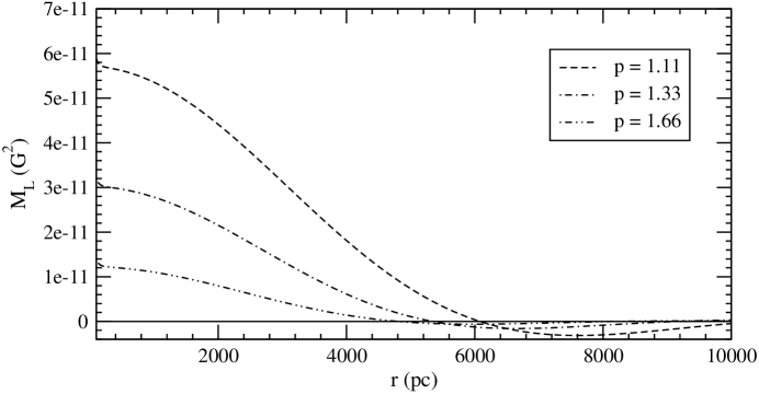
Figure 1: Final value of $M_{L}(\rm{G^{\,2}})$ as a function of $r(\rm{pc})$ for $p=1.11,1.33,$ and $1.66;$ $q=2;$ $L_{c}=81\,\rm{pc};$ $V_{c}=98\,\rm{km\,s^{-1}};$ and $a=9.76\times 10^{\,38}\,\rm{cm^{\,3}\,s\,g^{-1}}.$ We see that $B_{M}$ and $L_{M}$ are somewhat larger for smaller values of $p.$

In Figure 2, we show $M_{L}\left(r\right)$ as a function of $r$ for $q=1.8,$ $2,$ and $2.5,$ using $p=1.33$ and the same values for $L_{c},$ $V_{c},$ and $a$ as in Figure 1. The values of $B_{M}$ and $L_{M}$ are a little larger for smaller values of $q.$

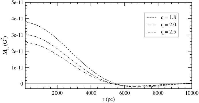
Figure 2: Final $M_{L}(\rm{G^{\,2}})$ as a function of $r(\rm{pc})$ for $q=1.5,2,$ and $2.5;$ $p=1.333;$ $L_{c}=81\,\rm{pc};$ $V_{c}=98\,\rm{{km}\,s};$ $a=9.76\times 10^{\,38}\,\rm{cm^{\,3}\,s\,g^{-1}};$ and ${p=1.33}.$ For smaller values of $q,$ $B_{M}$ and $L_{M}$ are somewhat larger.

In Figure 3, we plotted $M_{L}\left(r\right)$ as a function of $r$ for $a=3.2\times 10^{\,39}\;\rm{cm^{\,3}\,s\,g^{-1}},9.7\times 10^{\,39}\;\rm{cm^{\,3}\,s\,g^{-1}},$ and $2.43\times 10^{\,40}\;\rm{cm^{\,3}}\,s\,g^{-1};$ $p=1.33;$ and $q=2.$ We used the same values for $L_{c}$ and $V_{c}$ as in Fig. 1. We see that the smaller the value of $a$ (high ion density and/or high ion-neutral collision frequency), the larger the value of $B_{M}$. However, $L_{M}$ is almost insensitive to the value of $a$.

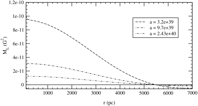
Figure 3: Final values of $M_{L}\rm({G^{\,2})}$ as a function of $r(\rm{pc})$ for $q=2,$ $p=1.333,$ $L_{c}=81\,\rm{pc},$ and $V_{c}=98\,\rm{{km}\,s^{-1}}$ and three different values for $a:$ $3.2\times 10^{\,38}\,\rm{cm^{\,3}}\,s\,g^{-1},$ $9.76\times 10^{\,38}\,\rm{cm^{\,3}\,s\,g^{-1}},$ and $2.43\times 10^{\,39}\,\rm{cm^{\,3}\,s\,g^{-1}}.$ For smaller values of $a$, $B_{M}$ is larger, while $L_{M}$ remains practically unchanged.

In Figure 4, we plotted $M_{L}\left(r\right)$ as a function of $r$ for $q=2,$ $p=1.33,$ $L_{c}=81\,\rm{pc},$ $a=3.2\times 10^{\,39}\,\rm{cm^{\,3}\,s\,g^{-1}},$ and $V_{c}=30\,\rm{km\,s^{-1}},$ $45\,\rm{km\,s^{-1}},$ and $96\,\rm{{km}\,s^{-1}}.$ We see that large values of these two parameters produce high values of $M_{L}$ as well as large coherence lengths.

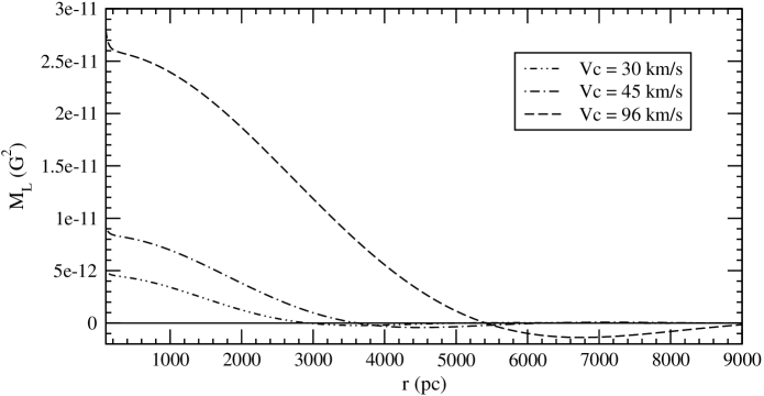
Figure 4: Final values of $M_{L}\rm{(G^{\,2}})$ as a function of $r(\rm{pc})$ for $q=2,$ $p=1.33,$ $L_{c}=81\,\rm{pc},$ and $a=9.76\times 10^{\,38}\,\rm{cm^{\,3}\,s\,g^{-1}}$ and three different values for $V_{c}$:$30\,\rm{km\,s^{-1}}$, $45\,\rm{km\,s^{-1}}$, and $96\,\rm{{km}\,s^{-1}}.$ We see that for larger values of $V_{c}$, $B_{M}$ and $L_{M}$ are larger.

Finally, in Figure 5, we plotted the evolution of $M_{L}$ as a function of $t$ at $r_{0}=112\;\rm{pc},$ going from $z=10$ to $z=5,$ for $M_{L}\left(r_{0},\,t=0\right)=1.5\times 10^{-38}\;\rm{G^{\,2}}$, $1.5\times 10^{-47}\;\rm{G^{\,2}},$ and $1.5\times 10^{-55}\;\rm{G^{\,2}}$. We see that after a short period of time, $t\sim 5\times 10^{\,6}\;\rm{years},$ $M_{L}$ reaches its saturation value, $M_{L}^{\,1/2}\sim 10^{-6}\;\rm{G},$ independent of its initial value.

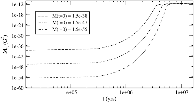
Figure 5: Values of $M_{L}\rm{(G^{\,2})}$ as a function of $t\rm{(years)}$ at $r_{0}=112\;\rm{pc}$ for three different initial values: $M_{L}\left(r_{0},t=0\right)=1.5\times 10^{-38}\,\rm{G^{\,2}},$ $1.5\times 10^{-47}\,\rm{G^{\,2}},$ and $1.5\times 10^{-55}\,\rm{G^{\,2}}.$ We used $p=1.11,$ $q=2,$ $L_{c}=81\,\rm{pc},$ $V_{c}=98\,\rm{km\,s},$ and $a=9.76\times 10^{\,38}\,\rm{cm^{\,3}\,s\,g^{-1}}.$ Independent of the initial values of $M_{L},$ saturation occurs at a time $t\sim 5\times 10^{\,6}\,\rm{years},$ when $M_{L}^{\,1/2}\sim 10^{-6}\,\rm{G}$.

Throughout the integration time, the kinetic energy density of the fluid was greater than that of the magnetic energy. The magnetic energy density is given by $E_{B}=B^{\,2}/8\,\pi,$ which for $B\sim 10^{-6}\;\rm{G}$ (see Fig. 5), has a value of $E_{B}\simeq 10^{-18}\;\rm{erg\,cm^{-3}}.$ The kinetic energy density is given by $E_{V}=\rho_{n}V_{c}^{\,2/}2.$ For $V_{c}=98\;\rm{km\,s^{-1}}$ and the range of values used for $\rho_{n},$ the kinetic energy, $3\times 10^{-13}\;\rm{erg\,cm^{-3}}$ $\lesssim E_{V}\lesssim 10^{-9}\;\rm{erg\,cm^{-3}},$ was many orders of magnitude greater than the magnetic energy.

4 CONCLUSIONS

In this work, we studied the problem of the origin of strong coherent large-scale magnetic fields, observed in low-redshift galaxies and previously thought to have been created by the mean field dynamo. Since doubts have been cast on the mean field dynamo as the source of these fields due to their observation in high redshift objects, where the dynamo would not have had suficient time to operate, we investigated here the stochastic helical dynamo as such a source. We showed that these fields can be generated in the plasmas found in very high redshift objects.

The generation of strong large scale coherent fields is a highly non-linear magnetohydrodynamical problem, which depends upon many factors. Here we discussed a possible mechanism for the generation of large scale fields, namely the non-linear evolution and diffusion of magnetic noise. Magnetic noise becomes coherent on a scale which is larger than that of the turbulence due to the presence of non linear terms in the evolution equations for the magnetic correlations.

We found that for realistic turbulent parameters, it is possible to generate the magnetic fields, observed at high redshifts . Between $z\sim 10$ and $z\sim 5$, the primordial plasma is strongly turbulent and partially ionized The magnetic field intensities reached are independent of initial correlations.

We considered a very simple model for the generation and evolution of the magnetic correlations. The dependence of the resulting magnetic field intensity on the charge composition of the primordial plasma, suggest that the reionization and star formation processes played an important role in determining the features of the magnetic fields detected in high redshift objects. In a forthcoming work we shall address the evolution of the magnetic correlations, considering a time dependent ion density as well as other nonlinear processes, such as the the Hall effect. Other turbulent scenarios, in addition to the homogeneous and isotropic one considered here, will be treated as well.

5 ACKNOWLEGEMENTS

We thank George Morales for useful comments. This work was partially supported by the Brazilian financing agency FAPESP (00/06770-2). A.K. acknowledges the FAPESP fellowship (01/07748-3). R. O. acknowledges partial support from the Brazilian financing agency CNPq (300414/82-0).

References

- Barkana & Loeb (2001) Barkana, R. & Loeb, A. 2001, Phys. Rep., 349, 125
- Blandford & Eichler (1987) Blandford, R. D. & Eichler, D. 1987, Phys. Rep., 154, 1
- (3) Brandemburg, A. & Subramanian, K. 2000, A&A, 361, L33
- Carrilli & Taylor (2002) Carrilli, C. L. & Taylor, R. B. 2002, ARA&A, 40, 319
- see reviews Grasso & Rubinstein (2001) Grasso, D. & Rubinstein, H. 2001, Phys. Rep., 348, 163
- (6) Kazantsev, A. P. 1968, JETP, 26, 1031
- Kulsrud & Anderson (1992) Kulsrud, R. M. & Anderson, S. W. 1992, ApJ, 396, 606
- (8) Lanzetta, K. M., Yahata, N., Pascarelle, S., Chen, H.-W., & Fernández-Soto, A. 2002, ApJ, 570, 492
- McComb (1990) McComb, W. D. 1990, The Physics of Fluid Turbulence (Oxford: Clarendon)
- Moffat (1978) Moffat, K. H. 1978, Magnetic Field Generation in Electrically Conducting Fluids (Cambridge: Cambridge Univ. Press)
- Monin & Yaglom (1975) Monin, A. S. & Yaglom, A. A. 1975, Statistical Fluid Mechanics, Vol. 2 Cambridge: MIT Press)
- NRL (2002) Naval Research Laboratory 2002, Plasma Formulary
- (13) Subramanian, K. 1999, Phys. Rev. Lett., 83, 2957
- Vainshtein (1982) Vainshtein, S. I. 1982, JETP, 56, 86
- (15) Vainshtein S. I. & Kichatinov, L. L. 1986, JFM, 168, 73
- (16) Völk, H. J., Klein, U., & Wielebinski, R. 1989, A&A, 213, L12
- Widrow (2002) Widrow, L. M. 2002, Rev. Mod. Phys., 74, 775
- Zel’dovich et al. (1983) Zel’dovich, Ya. B., Ruzmaikin, A. A., & Sokoloff, D. D. 1983, Magnetic Fields in Astrophysics (New York: Gordon & Breach)
- Wolfe et al. (1992) Wolfe, A. M., Lanzetta, K. M., & Oren, A. L. 1992, ApJ, 388, 17