Gamma-Ray Burst Intensity Distributions

Abstract

We use the lag-luminosity relation to calculate self-consistently the redshifts, apparent peak bolometric luminosities $L_{B}$, and isotropic energies $E_{\rm iso}$ for a large sample of BATSE gamma-ray bursts. We consider two different forms of the lag-luminosity relation; for both forms the median redshift for our burst database is 1.6. We model the resulting $E_{\rm iso}$ sample with power law and Gaussian probability distributions without redshift evolution, both of which are reasonable models. The power law model has an index of $\alpha_{E}=1.76\pm 0.05$ (95% confidence), where $p(E_{\rm iso})\propto E_{\rm iso}^{-\alpha_{E}}$. The simple universal jet profile model suggested but did not require $\alpha_{E}=2$, and subsequent physically reasonable refinements to this model permit greater diversity in $\alpha_{E}$, as well as deviations from a power law; therefore our observed $E_{\rm iso}$ probability distribution does not disprove the universal jet model.

1 Introduction

The major breakthroughs in the study of gamma-ray bursts of the past six years—most if not all bursts are cosmological, bursts do not have constant peak luminosity, the fireballs are beamed, many bursts are associated with supernovae—resulted from the intensive study of a relatively small number of bursts without regard for whether these bursts formed a well defined statistical sample. However, realizing that for any one burst we are only sampling an anisotropic radiation pattern from one direction, we now have to study distributions of burst properties to reconstruct the bursts’ appearance from all directions. Well-defined burst samples are required to derive these distributions.

Unfortunately, we do not yet have a large sample of bursts with spectroscopic redshifts, which in most cases are required for calculating the intrinsic burst properties. The two dozen or so bursts with redshifts were detected by various detectors with different detection thresholds and energy sensitivities, and the follow-ups that determined the redshifts depended on the vagaries of weather and telescope availability. BATSE provided a large burst sample with well-understood thresholds, but without direct redshift determinations for most of these bursts. However, redshifts can be determined indirectly from the lag-luminosity (Norris, Marani & Bonnell 2000) or variability-luminosity (Fenimore & Ramirez-Ruiz 2000; Reichart et al. 2001) relations. Here we calculate self-consistently the redshifts for a large subset of the BATSE bursts using the lag-luminosity relation. To accommodate the problematic burst GRB980425, which is significantly underluminous if the lag-luminosity relation is a single power law, Salmonson (2001) and Norris (2002) proposed that the relation should be a broken power law. This reduces the luminosity of many long-lag bursts, moving this population closer to the observer.

We use the resulting redshifts to calculate both the peak bolometric luminosity $L_{B}$ and the isotropic energy $E_{\rm iso}$. Bursts are thought to radiate anisotropically, but we sample their radiation field in only one direction. Therefore $L_{B}$ and $E_{\rm iso}$ are calculated from the observed flux as if the emissions are isotropic; corrections for the anisotropy are based on models of the relativistic jets that emit the observed gamma rays (see Bloom, Frail & Kulkarni 2003). $L_{B}$ and $E_{\rm iso}$ are both bolometric quantities in the burst frame. $L_{B}$ is the maximum value of the luminosity while $E_{\rm iso}$ is the total energy emitted over the duration of the burst (without correcting for the anisotropic emission). We consider the isotropic energy $E_{\rm iso}$ to be more fundamental, and therefore model its probability distribution.

Two models have been proposed for the structure of the jets. The uniform jet model (Frail et al. 2001; Bloom et al. 2003) assumes that all jets have a constant surface energy density $\epsilon$ (energy per solid angle across the jet) but differing opening angles $\theta_{0}$ (the angle between the jet axis and the edge of the jet). The model makes no predictions for the energy probability distribution. On the other hand, in the universal jet profile model (Rossi, Lazzati, & Rees 2002; Zhang & Meszaros 2002) all jets have the same surface energy density $\epsilon$ as a function of off-axis angle $\theta$ (the angle from the jet axis), and thus the observed differences in $L_{B}$ or $E_{\rm iso}$ result from the angle $\theta_{v}$ between the jet axis and the line-of-sight. This model predicts that the energy probability distribution is a power law with index $\alpha_{E}$, where $p(E_{\rm iso})\propto E_{\rm iso}^{-\alpha_{E}}$. If $\epsilon\propto\theta^{k}$, then $\alpha_{E}=1-2/k$. Rossi et al. (2002) and Zhang & Meszaros (2002) suggested $k=-2$, resulting in $\alpha_{E}=2$, to reproduce the distributions observed by Frail et al. (2001), although this was not a firm prediction. A Gaussian surface energy density profile results in $\alpha_{E}=1$ (Lloyd-Ronning, Dai & Zhang 2004). Thus $\alpha_{E}$ is of order 1–2. Lloyd-Ronning et al. (2004) showed that allowing the parameters of the jet profile to vary somewhat from burst to burst—the jet profile is now only quasi-universal—results both in variations in the value of $\alpha_{E}$ and deviations from a pure power law. While numerical modelling of hypernovae (Zhang, Woosley, & MacFadyen 2003) shows that the surface energy density of the outflows should vary with off-axis angle, it does not predict the profile; thus the profiles are fitted empirically to the data. Consequently, the observed $E_{\rm iso}$ probability distribution is not a powerful discriminant between the two jet structure models.

This paper has two goals. First, we calculate the redshift of a large sample of bursts self-consistently from the lag-luminosity relation. With the redshift and the observed fluxes and fluences we calculate $L_{B}$ and $E_{\rm iso}$. Second, we model the $E_{\rm iso}$ distribution with two functional forms: power law and lognormal. We find the best fit values for the parameters of each functional form, and evaluate how well each functional form describes the data. We also compare the fit of the power law functional form to the predictions of the universal jet profile model.

In these calculations we use a cosmology with $H_{0}=70$ km s^-1 Mpc^-1, $\Omega_{m}=0.3$ and $\Omega_{\Lambda}=0.7$. The notation $p(a\,|\,b)$ means the probability of $a$ given $b$. Lower case $p$ denotes a probability density while upper case $P$ (without a subscript) represents a cumulative probability. Note that $a$ and $b$ are propositions that are true or false. A proposition can be a statement such as “the energy distribution can be described with a lognormal functional form” or a parameter value (equivalent to the statement “the parameter value is 5”).

In §2 we present the methodology used in this study: calculating the burst redshifts (§2.1); fitting the energy probability distribution (§2.2); and using the cumulative probability to test the quality of the fit (§2.3). The implementation of this methodology is discussed in §3 and the results are provided by §4. Finally, our conclusions are in §5.

2 Methodology

2.1 Calculating Redshifts

In the absence of a large number of measured spectroscopic redshifts, we use the lag-luminosity relation (Norris et al. 2000) to calculate peak luminosities $L_{B}$, and subsequently redshifts, for a large burst sample. Assume that for a set of bursts we have measured the lag $\tau_{0}$ (s) between the light curves in two energy bands, the peak photon flux $P_{\rm ph}$ (ph s^-1 cm^-2) in the photon energy band $E_{L}$–$E_{U}$, and the spectral fit for the time period over which $P_{\rm ph}$ is measured. The spectral fit ($N_{\rm ph}(E)$—ph cm^-2 s^-1 keV^-1) uses the “Band” functional form (Band et al. 1993) which is characterized by an asymptotic low energy power law with index $\alpha$ ($N_{\rm ph}(E)\propto E^{\alpha}$), a high energy power law with index $\beta$ ($N_{\rm ph}(E)\propto E^{\beta}$), and a characteristic energy $E_{p}$ between the two power laws; for $\beta<-2$ $E_{p}$ is energy at the peak of the $E^{2}N_{\rm ph}$ (energy per logarithmic frequency interval) light curve. This functional form is fitted to the observed count spectrum, which covers a limited energy range, but is extrapolated to high and low energy, as needed. The instrument team is assumed to have converted the observed peak count rate into the peak photon flux using the fitted spectral model and the response function.

The lag $\tau_{B}$ in the burst’s frame and the observed lag $\tau_{0}$, both between the same energy bands in their respective frames, are related by time dilation (which increases the lag) and spectral redshifting (which shifts the smaller lag at high energy into the observed band). The first effect is simple and universal—a factor of $(1+z)^{-1}$. The second depends on the burst’s spectral evolution, and may vary from burst to burst. Thus

$$\tau_{B}=\tau_{0}g(z)\quad.$$ (1)

We assume that $g(z)$ is universal, and as a working assumption we use $g(z)=(1+z)^{c_{\tau}}$. Time dilation contributes $-1$ to $c_{\tau}$, while the redshifting of temporal structure with a smaller lag from higher energy contributes a positive constant (e.g., $\sim 1/3$; Fenimore et al. 1995 found $\sim 0.4$).

Empirically the lag has been related to the apparent bolometric peak luminosity $L_{B}$ (erg s^-1; Norris et al. 2000)

$$L_{B}=Q(\tau_{B})\quad.$$ (2)

The observed peak bolometric energy flux $F_{B}$ (erg cm^-2 s^-1) is related to the bolometric peak luminosity $L_{B}$ through the redshift, and an assumed cosmology:

$$F_{B}=L_{B}/[4\pi D_{L}^{2}]\quad,$$ (3)

where $D_{L}$ is the luminosity distance. Note that $L_{B}$ is the “isotropic” peak bolometric luminosity, the peak luminosity if the observed flux were beamed in all directions. If the flux is actually beamed into a solid angle $\Delta\Omega$, then the actual peak luminosity is only $\Delta\Omega/4\pi$ of $L_{B}$. We define

$$\langle E\rangle = F_{B}/P_{\rm ph}$$ (4)

$$\hbox{where}\quad P_{\rm ph} = \int_{E_{L}}^{E_{U}}N_{\rm ph}(E)dE$$ (5)

$$\hbox{and}\quad F_{B} = \int_{0}^{\infty}EN_{\rm ph}(E)dE\quad;$$ (6)

$N_{\rm ph}(E)$ is the photon spectrum. The photon spectrum energy flux $F_{B}$ results from a fit to the observed spectrum which is available over a limited energy band from a time bin that includes the peak of the light curve. Thus the peak bolometric energy flux $F_{B}$ is calculated by extrapolating $N_{\rm ph}(E)$ in eq. 6 to high and low energies.

The resulting implicit equation for redshift,

$$P_{\rm ph}={{Q\left(\tau_{0}g(z)\right)}\over{4\pi D_{L}^{2}\langle E\rangle}}\quad,$$ (7)

must be solved for each burst. The inputs are $\tau_{0}$, $P_{\rm ph}$ and $\langle E\rangle$ (which is calculated from the spectral fit). The functional form of the lag-luminosity relation $Q$ is calibrated from the small set of bursts for which $z$ is known. We have an assumed functional form for $g(z)$ with one unknown constant $c_{\tau}$. This constant can be calculated using the dependence of $\tau$ on energy bands (Fenimore et al. 1995).

These equations can be evaluated for the sensitivity of calculated quantities such as $z$ and $L_{B}$ on observables such as $P_{\rm ph}$ and $\langle E\rangle$ (which, in turn, depends on the spectral parameters). Eq. 7 shows that $z=\phi(P_{\rm ph}\langle E\rangle,\tau_{0})$ while eqs. 3–4 can be combined to give $L_{B}=P_{\rm ph}\langle E\rangle\psi(z)$, where $\phi$ and $\psi$ are functions defined only for this sensitivity analysis and need not be derived explicitly. The quantities $P_{\rm ph}$ and $\langle E\rangle$ appear in these expressions only in the product $P_{\rm ph}\langle E\rangle$, and consequently errors in $\langle E\rangle$, resulting from uncertainties in the spectral parameters, are equivalent to errors in $P_{\rm ph}$. As shown by figure 1, these equations give curves in $z$–$L_{B}$ space parameterized by $\tau_{0}$; larger values of the product $P_{\rm ph}\langle E\rangle$ lie at larger values of $z$ and $L_{B}$ on the appropriate curve.

If the spectrum is fairly flat, e.g., $\alpha=-1$ and $\beta=-2$, then $\langle E\rangle$ does not vary by a large factor as $E_{p}$ varies. The segments plotted on figure 1 are for $E_{p}$ ranging between 5 keV and 2 MeV for $\alpha=-1$ and $\beta=-2$ while holding $P_{\rm ph}$ fixed. However, if the spectrum is more peaked, i.e., is harder at low energies (larger $\alpha$) or softer at high energy (smaller $\beta$), then the $\langle E\rangle$ range is larger. This is shown on figure 1 by the diamonds, triangles and asterisks that mark the range that results as $E_{p}$ varies for different sets of $\alpha$ and $\beta$. As can be seen, cavalier treatment of the spectrum of the peak flux can result in large errors in $z$ and $L_{B}$.

Solving eq. 7 provides $z$ for each burst (note that $L_{B}$ does not appear explicitly in eq. 7). With $P_{\rm ph}$ and the energy fluence (erg cm^-2) we then calculate $L_{B}$ and $E_{\rm iso}$. The result is a large database of observables (lags, $P_{\rm ph}$, energy fluences, spectral parameters) and derived quantities ($z$, $L_{B}$, and $E_{\rm iso}$) with which we can address different questions about the burst population. Here we study the distribution of intensity measures such as $L_{B}$ and $E_{\rm iso}$.

2.2 The Intensity Probability Distribution

We use a Bayesian analysis to investigate intensity probability distributions, although we argue that a frequentist analysis will give the same result; Band (2001) provides a more complete exposition of the methodology. In this study we consider the isotropic energy $E_{\rm iso}$ as the relevant intensity measure; the same formulae apply substituting $L_{B}$ for $E_{\rm iso}$.

Our burst database provides the isotropic energy $E_{\rm iso}$, the peak photon flux $P_{\rm ph}$ and the redshift $z$ for each burst. The threshold peak flux $P_{\rm ph,min}$ is known, from which the threshold isotropic energy $E_{\rm iso,min}$ for each burst is calculated: $E_{\rm iso,min}=E_{\rm iso}\,P_{\rm ph,min}/P_{\rm ph}$. The energy probability distribution function is the normalized probability distribution $p(E_{\rm iso}\,|\,\vec{a_{j}},M_{j},I)$ where $\vec{a_{j}}$ is the set of parameters that characterize the $j$th model distribution function represented by $M_{j}$, and $I$ specifies general assumptions about our calculation. Thus $M_{j}$ states that we are using the $j$th functional form, which has parameters $\vec{a_{j}}$. There are always additional assumptions upon which the calculation rests, such as the underlying cosmology or the detector calibration. The validity of our analysis depends on these assumptions, which we represent with the proposition $I$. If the distribution evolves with redshift, then $z$ should be included in the list of ‘givens’ in the probability distribution; here we do not include a redshift dependence. Thus we do not consider redshift evolution in our analysis. Because we work with probability distributions that are normalized at each redshift, our results remain valid for evolution in the burst rate per comoving volume.

In our calculations we use power law and lognormal energy probability distributions. In the power law case the proposition $M_{j}=M_{\rm pl}$ is the statement that the functional form is a power law, and the parameters $\vec{a_{j}}$ are the power law index $\alpha_{E}$ and the low energy cutoff $E_{2}$:

$$p(E_{\rm iso}\,|\,\alpha_{E},E_{2},M_{\rm pl},I)\propto E_{\rm iso}^{-\alpha_{E}}\qquad\hbox{for}\qquad E_{\rm iso}\geq E_{2}\quad.$$ (8)

For a finite number of bursts the distribution must have a low energy cutoff $E_{2}$ if $\alpha_{E}>1$. As we will see, the fit to the power law model is relatively insensitive to the low energy cutoff $E_{2}$. Therefore our results are valid for redshift evolution in the energy scale (i.e., in $E_{2}$), but not in the power law index.

In the lognormal case $M_{j}=M_{\ln}$ states that the functional form is a lognormal, and the parameters are the energy centroid $E_{\rm iso,cen}$ and the logarithmic width $\sigma_{E}$:

$$p(E_{\rm iso}\,|\,E_{\rm iso,cen},\sigma_{E},M_{\rm ln},I)={1\over{\sqrt{2\pi}\sigma_{E}}}\exp\left[{{\left(\ln\left(E_{\rm iso}\right)-\ln\left(E_{\rm iso,cen}\right)\right)^{2}}\over{2\sigma_{E}^{2}}}\right]\quad.$$ (9)

For the $i$th burst we have $E_{\rm iso,i}$ with threshold $E_{\rm iso,min,i}$, the set of which constitutes the data $D$. The observed $E_{\rm iso,i}$ are not drawn from $p(E_{\rm iso}\,|\,\vec{a_{j}},M_{j},I)$ but from

$$p(E_{\rm iso}\,|\,E_{\rm iso,min},\vec{a_{j}},M_{j},I)={{p(E_{\rm iso}\,|\,\vec{a_{j}},M_{j},I)H(E_{\rm iso}-E_{\rm iso,min})}\over{\int_{E_{\rm iso,min}}^{\infty}dE_{\rm iso}\,p(E_{\rm iso}\,|\,\vec{a_{j}},M_{j},I)}}$$ (10)

where $H(x)$ is the Heaviside function (1 for positive $x$ and 0 for negative $x$); $E_{\rm iso}$ is drawn from the observable part of the energy distribution function.

The probability of obtaining the data $D$ given the model is the ‘likelihood’

$$\Lambda_{j}=p(D\,|\,\vec{a_{j}},M_{j},I)=\prod_{i=1}^{N_{B}}p(E_{\rm iso,i}\,|\,E_{\rm iso,min,i},\vec{a_{j}},M_{j},I)$$ (11)

where the product is over the $N_{B}$ bursts in our database. In the “frequentist” framework best-fit parameters are typically found by maximizing $\Lambda_{j}$ through varying the parameters. Plotting $\Lambda_{j}$ as a function of $\vec{a_{j}}$ around the maximum reveals the range of acceptable $\vec{a_{j}}$ values.

However the Bayesian analysis is based on $p(\vec{a_{j}}\,|\,D,M_{j},I)$, the posterior probability for the parameters, that is, the probability that the particular set of $\vec{a_{j}}$ values is correct given the data. Bayes theorem gives

$$p(\vec{a_{j}}\,|\,D,M_{j},I)={{p(D\,|\,\vec{a_{j}},M_{j},I)p(\vec{a_{j}}\,|\,M_{j},I)}\over{\int d\vec{a_{j}}\,p(D\,|\,\vec{a_{j}},M_{j},I)p(\vec{a_{j}}\,|\,M_{j},I)}}\quad.$$ (12)

The factor $p(\vec{a_{j}}\,|\,M_{j},I)$ is the prior for $\vec{a_{j}}$, constraints on the parameters based on information available before the new data were acquired. The factor in the denominator is a normalizing constant. Thus for parameter determination the Bayesian approach explicitly factors in additional information and constraints (e.g., energies must be non-negative and finite). The expectation value of the parameters is

$$\langle\vec{a_{j}}\rangle=\int d\vec{a_{j}}\,\vec{a_{j}}\,p(\vec{a_{j}}\,|\,D,M_{j},I)\quad.$$ (13)

If $\Xi_{j}=p(D\,|\,\vec{a_{j}},M_{j},I)p(\vec{a_{j}}\,|\,M_{j},I)$, the numerator in eq. 12, is sharply peaked, then the expectation value of the parameters occurs at the peak of $\Xi_{j}$. However the posterior probability $p(\vec{a_{j}}\,|\,D,M_{j},I)$ (or $\Xi_{j}$) is required to determine the acceptable parameter range.

As was discussed in Band (2001), reasonable priors for the parameters of both the power law and lognormal distributions are constants (when the logarithm of an energy is treated as the parameter rather than the energy), and therefore the frequentist likelihood $\Lambda_{j}$ and the Bayesian posterior $p(\vec{a_{j}}\,|\,D,M_{j},I)$ are proportional to each other. Consequently, while we favor the Bayesian approach, here the frequentist and Bayesian analyses are the same. We calculate $\Lambda_{j}$ as a function of the parameters $\vec{a_{j}}$. The maximum of $\Lambda_{j}$ gives the best fit parameter values while the width of $\Lambda_{j}$ shows the range of acceptable values, and correlations between the parameter values.

Note that the methodology we use here only provides the normalized probability distribution, not the normalization of the distribution (i.e., the burst rate per volume). The normalization requires the history of $E_{\rm iso,min}$ during the mission (i.e., not only for the detected bursts).

2.3 The Cumulative Probability

The Bayesian approach does not provide a goodness-of-fit statistic. However a frequentist statistic can be derived. For each burst the cumulative probability is

$$P(>E_{\rm iso,i}\,|\,E_{\rm iso,min,i},\vec{a_{j}},M_{j},I)=\int_{E_{\rm iso,i}}^{\infty}p(E_{\rm iso}\,|\,E_{\rm iso,min,i},\vec{a_{j}},M_{j},I)\,dE_{\rm iso}\quad.$$ (14)

If the assumed energy distribution function is an acceptable characterization of the observations (which would be the case if the model $M_{j}$ is correct) and all the assumptions (included in the proposition $I$) are valid (e.g., the cosmological model is correct), then the cumulative probabilities $P(>E_{\rm iso,i})$ for each burst should be uniformly distributed between 0 and 1, and have an average value of $\langle P(>E_{\rm iso,i})\rangle=1/2\pm(12N_{B})^{-1/2}$ for the $N_{B}$ bursts in the sample. Note that $(12N_{B})^{-1/2}$ is the expected statistical variance resulting from the size of the sample, and does not take into account systematic errors.

3 Implementation

3.1 Datasets

We start with a database for 1438 BATSE bursts that includes the lags and their uncertainties, the peak flux $P_{\rm ph}$ over the 50–300 keV band on the 256 ms timescale, the burst duration $T_{90}$, and hardness ratios among the 4 BATSE energy channels (30–50, 50–100, 100–300, and 300–2000 keV). Of these 1438 bursts, 1218 have positive lags.

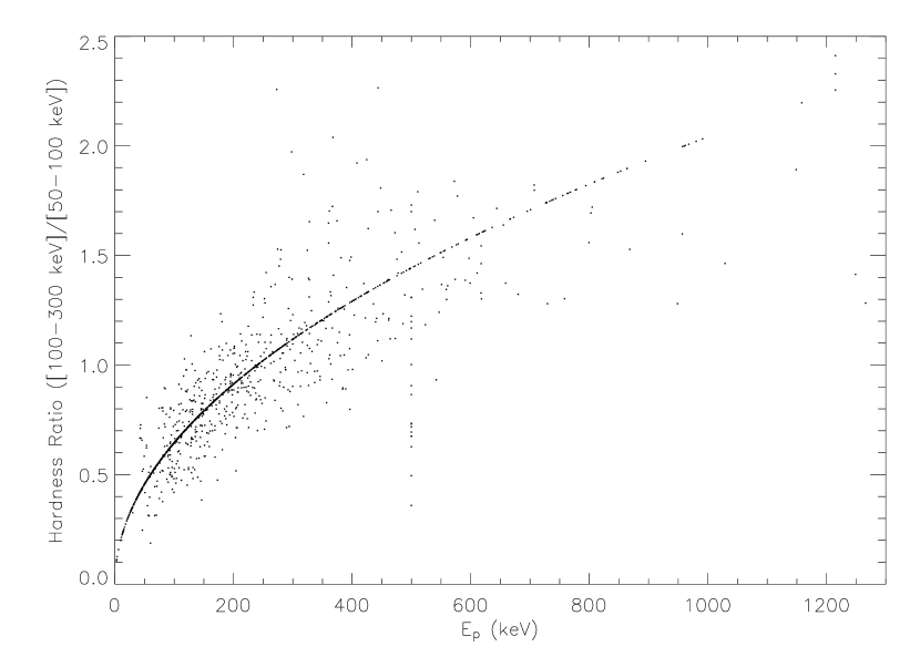
Figure 2: Hardness ratio HR₃₂ (100–300 keV vs. 50–100 keV) as a function of $E_{p}$. Two populations are evident. First, spectral fits were not available for the bursts that fall on an empirical $E_{p}\propto\hbox{HR}_{32}^{2}$ relation. Second, bursts with spectral fits are dispersed around this $E_{p}\propto\hbox{HR}_{32}^{2}$ relation.

To calculate the average energy $\langle E\rangle$ (see eq. 4) we use the parameters of the “Band” spectrum fits by Mallozzi et al. (1998) to the 16 channel BATSE “CONT” count spectra accumulated over the peak flux time interval (usually 2.048 s) for the 580 bursts in our database that are also in the Mallozzi et al. database. For the 858 bursts that are not in the Mallozzi et al. database we assume the average low and high energy spectral indices of $\alpha=-0.8$ and $\beta=-2.3$ found by Preece et al. (2000). Because $E_{p}$, the energy of the peak of the $E^{2}N_{\rm ph}(E)\quad(\propto\nu f_{\nu})$ curve, and HR₃₂, the 100–300 keV to 50–100 keV hardness ratio, are strongly correlated, we use the empirical relation $E_{p}$ = 240 HR${}_{32}^{2}$ keV (for HR${}_{32}\leq 2.25$) for the bursts without spectral fits. In §2.1 we discussed the sensitivity of $z$ to errors in the spectrum; the gaps in the available spectral fits introduces a systematic uncertainty into our analysis. Figure 2 shows the resulting scatter plot for $E_{p}$ vs. HR₃₂.

3.2 The Lag-Luminosity Relation

Based on less than a dozen bursts, Norris et al. (2000) found that $L_{B}\propto\tau_{B}^{-1.15}$. However, this single component relationship predicts a much greater $L_{B}$ than observed for GRB980425, the burst that appears to coincide with the supernova SN1998bw. By introducing a break in the lag-luminosity relation Salmonson (2001) and Norris (2002) were able to include GRB980425. The resulting lag-luminosity relation is:

$$L_{51}=2.18(\tau_{B}/0.35\hbox{ s})^{c_{L}},\quad c_{L}=-1.15\hbox{ for $\tau_{B}\leq 0.35$ s, }-4.7\hbox{ for $\tau_{B}>0.35$ s.}$$ (15)

where $L_{51}=L_{B}/10^{51}$ erg s^-1. In our calculations we use both the single (i.e., $c_{L}=-1.15$ for all $\tau_{B}$) and two component lag-luminosity relations.

4 Results

4.1 Lag-Luminosity Relation and Redshift

We first investigate the lag-luminosity relation and then use it to construct a database of burst redshifts, $L_{B}$ and $E_{\rm iso}$. Salmonson (2001) and Norris (2002) introduced a break in the simple power law relation to include the long lag, very low luminosity GRB980425. As a result of this break other long lag bursts in the BATSE database are assigned low luminosities, and consequently small distances; Norris (2002) suggested that there may be a population of nearby low luminosity bursts. Figure 3 demonstrates this: the solid line is the cumulative distribution of burst redshifts assuming a single power law lag-luminosity relation, while the dashed line shows the distribution for the broken power law relation. Introducing a break in the power law shifts the low redshift bursts closer (i.e., to lower redshifts). Note this break was introduced only to include GRB980425 in the lag-luminosity relation; if GRB980425 was not associated with SN1998bw or if GRB980425 was anomalous, then this break is unnecessary and unsupported by other data.

Figure 3 also shows that there are few bursts with $z>10$. These bursts may indeed be at high redshift; finding such high redshift bursts is one of the goals of the Swift mission. However, on theoretical grounds bursts with $z>17$ are not expected. Given the dispersion in the lag-luminosity relation and the errors in determining $\tau_{0}$, it is not surprising that some bursts are assigned redshifts as high as $z=65$; large redshifts result from high luminosities for bursts with very small lags, which are particularly difficult to measure accurately. Thus the lag-luminosity relation does not give unphysical results at the high luminosity end. Norris (2002) placed an upper limit on the luminosity when he found a large number of very high redshift bursts.

We use the simple single power law lag-luminosity relation without any cutoffs or limits in the following analysis.

For our database the median redshift is $z_{m}=1.58$. As can be seen from Figure 3, this redshift is greater than the redshift range where the form of the lag-luminosity relation makes a difference.

Figure 4 shows the distribution of $L_{B}$ we calculate (the scatter plot) along with the threshold of $L_{B}$ at different redshifts (the lines). In calculating the threshold values of $L_{B}$ we assume a constant $P_{\rm ph,min}=0.3$ ph cm^-2 s^-1 and vary $\langle E\rangle$ (see eq.  4). Factor of $\sim 3$ differences in $\langle E\rangle$ result in significant over- or under-predictions of the threshold.

Thus we have accomplished the first goal of this paper. The resulting database is provided online at http://cossc.gsfc.nasa.gov/analysis/lags/ .

4.2 The $E_{\rm iso}$ Probability Distribution

We focus on the probability distribution functions of the bolometric energy. To perform quantitative estimates of distributions as a function of redshift (e.g., of the burst rate) the threshold for the database must be known, and therefore studies have often focused on the peak luminosity $L_{B}$; $L_{B}$ is more closely related to the peak flux $P_{\rm ph}$, which has a relatively sharp instrumental threshold $P_{\rm ph,min}$. However, to study probability distributions of intrinsic burst quantities the threshold for that quantity for each observed burst will suffice. Thus our database is sufficient to study both the isotropic energy $E_{\rm iso}$ and the peak luminosity $L_{B}$ probability distributions.

Figure 5 shows the scatter plot of the isotropic energy $E_{\rm iso}$. The region just above the threshold is underpopulated, suggesting that the thresholds are underestimated for this database. Therefore, we raise the threshold to $P_{\rm ph,min}=0.5$ ph cm^-2 s^-1, raising the median redshift from 1.58 to 1.62, and decreasing the number of bursts to 1054.

4.2.1 Power Law $E_{\rm iso}$ Distribution

This functional form is relevant because it is predicted by the universal jet profile model. Figure 6 shows the resulting likelihood surface, which peaks at $\alpha_{E}=1.76$ and $\log(E_{2})=50.2$. This value of $E_{2}$ is the smallest value of $E_{\rm iso}$ in our sample; burst samples that extend to fainter bursts will probably have smaller observed values of $E_{\rm iso}$, and consequently $E_{2}$ is most likely smaller. The contour plot indicates that the determination of $\alpha_{E}$ is independent of the value of $E_{2}$. Since the likelihood peaks at the same $\alpha_{E}$ at any given $E_{2}$, our result holds even if the energy scale evolves with redshift. The 95% confidence region centered on $\alpha_{E}=1.76$ has a half width of 0.05.

As discussed in §1, the universal jet profile model, especially with physically reasonable refinements, does not predict definitively a value of $\alpha_{E}$ that can then be used to falsify this model. Originally $\alpha_{E}=2$ was suggested (Rossi et al. 2002, Zhang & Meszaros 2002) for a surface energy density that is a power law in the jet off-axis angle, while a Gaussian surface energy density would have $\alpha_{E}=1$ (Lloyd-Ronning et al. 2004). Consequently our value of $\alpha_{E}=1.76\pm 0.05$ falls in the range of expected $\alpha_{E}$ values. Thus our work does not distinguish between the universal jet profile model and the uniform jet model (which does not predict an energy probability distribution).

Since the value of $\alpha_{E}$ is relevant to jet models, consideration of the possible systematic errors is warranted. Our method for estimating the energy probability distribution considers where each measured $E_{\rm iso}$ falls between $E_{\rm iso,min}$ for that burst and infinity. If $E_{\rm iso,min}$ is underestimated, then the low $E_{\rm iso}$ portion of the probability distribution will be under-represented, causing the distribution to be shifted to higher energy, in this case resulting in a smaller value of $\alpha_{E}$. Indeed, when we use $P_{\rm ph,min}$=0.1, 0.3, 0.5, 1 and 2 ph cm^-2 s^-1 we find $\alpha_{E}$=1.125, 1.6, 1.76, 1.9 and 2. Next, uncertainties in the measured value of $E_{\rm iso}$ that are symmetric to higher and lower values will cause a net ‘diffusion’ towards higher $E_{\rm iso}$ because there are more bursts below than above any given value of $E_{\rm iso}$. This effect also decreases $\alpha_{E}$. Note that small lags are more difficult to measure, resulting in greater uncertainties for large $L_{B}$; since $E_{\rm iso}$ is correlated with $L_{B}$ (but is not strictly proportional), on average the uncertainty increases for larger $E_{\rm iso}$. Therefore, the true value of $\alpha_{E}$ is most likely greater than the value we measured.

The likelihood alone does not indicate whether the power law model is a good description of energy distribution. The average of the cumulative probability (§2.3) should be $\langle P(>E_{\rm iso})\rangle=1/2\pm(12N_{B})^{-1/2}$ for $N_{B}$ bursts. Figure 7 shows that the cumulative $P(>E_{\rm iso})$ for $P_{\rm ph,min}=0.5$ ph cm^-2 s^-1 is very close to the straight line that is expected if the distribution function is a good description of the data. We calculate $\langle P(>E_{\rm iso})\rangle=0.4642$ with an expected statistical variance of $0.0089$ ($N_{B}=1054$). Thus $\langle P(>E_{\rm iso})\rangle$ differs from the expected value of 1/2 by $4\sigma$ using the statistical variance only. However, since the likely systematic uncertainties (e.g., in the value of $P_{\rm ph,min}$, in the determination of the lags, in the corrections for the redshifting of high energy light curves) are likely to be considerable, this value of $\langle P(>E_{\rm iso})\rangle$, and the proximity of the $P(>E_{\rm iso})$ distribution to a straight line (Figure 7), indicates that a power law is a good representation of the distribution.

4.2.2 Lognormal $E_{\rm iso}$ Distribution

The second model distribution we consider is a lognormal energy probability distribution; the parameters are the energy centroid $E_{\rm iso,cen}$ and the logarithmic width $\sigma_{E}$ of the distribution. For this distribution the likelihood (relevant to a frequentist analysis) and the posterior distribution as a function of $\ln E_{\rm iso,cen}$ and $\sigma_{E}$ (relevant to a Bayesian analysis) are the same if the prior is constant in $\ln E_{\rm iso,cen}$ and $\sigma_{E}$ (see Band 2001). Figure 8 shows the likelihood surface; the peak occurs at $E_{\rm iso,cen}=2.8\times 10^{50}$ ergs and $\sigma_{E}=2.7$. However, these parameters are highly correlated since a broader distribution (larger $\sigma_{E}$) can compensate for a smaller central energy $E_{\rm iso,cen}$. The figure shows that 95% of the probability distribution is in the range $E_{\rm iso,cen}=$(0.03–1)$\times 10^{51}$ erg and $\sigma_{E}=2.3$–3.2. As can be seen from figure 5, $E_{\rm iso,cen}=2.8\times 10^{50}$ ergs is at the lower end of the distribution of measured $E_{\rm iso,min}$, and thus the data are insufficient to determine whether the probability density does indeed decrease below $E_{\rm iso,cen}$.

For $P_{\rm ph,min}=0.5$ ph cm^-2 s^-1, $\langle P(>E_{\rm iso})\rangle=0.4821\pm 0.0089$ ($N_{B}=1054$), which is consistent with $\langle P(>E_{\rm iso})\rangle=1/2$ at the $2\sigma$ level. Note that for $P_{\rm ph,min}=0.3$ ph cm^-2 s^-1 $\langle P(>E_{\rm iso})\rangle=0.4598\pm 0.0085$ ($N_{B}=1162$), which differs from the expected value by nearly $5\sigma$ using the statistical variance only. As we argued above, there are undoubtedly significant systematic uncertainties in addition to the statistical variance. Figure 9 shows the distribution of the cumulative probability for $P_{\rm ph,min}=0.5$ ph cm^-2 s^-1; as can seen, the observed cumulative probability distribution is very close to the expected distribution. Again, considering the systematic uncertainties in our calculation, the lognormal distribution is consistent with the data.

4.2.3 Comparison to Previous Probability Distribution Calculations

In this study we apply the same methodology presented in Band (2001) to a new burst data set. In both studies the $E_{\rm iso}$ distributions are modelled with lognormal and power law functional forms, although Band (2001) applied a high energy cutoff to the power law function because in some cases $\alpha_{E}\leq 1$. Band (2001) used three data sets: a) ‘B9’—9 bursts with spectroscopic redshifts (i.e., the redshifts were measured from emission or absorption lines) and fitted BATSE spectra; b) ‘C17’—17 bursts with spectroscopic redshifts and spectral information from a variety of sources; and c) ‘F220’—220 bursts with redshifts derived from the variability-luminosity relation (Fenimore & Ramirez-Ruiz 2000). Table 1 presents the resulting parameters; 90% uncertainties are indicated. The variables of the lognormal distribution are highly correlated, resulting is large uncertainty ranges for both parameters. We find that as the database size increases, it samples smaller $E_{\rm iso}$, as can be seen from the values of $E_{2}$. Perhaps as a consequence, $E_{\rm iso,cen}$ decreases and $\alpha_{E}$ increases as the database size increases.

The distributions for these different samples are discrepant, which may result from systematic difficulties with the burst samples or incorrect assumed probability distribution functional forms. The variability-luminosity relation used for the F220 sample and the lag-luminosity relation used in this paper were both calibrated with only a few bursts, and the validity of these relations must be confirmed by a larger burst sample. The B9 and C17 samples use spectroscopic redshifts, and thus are affected by selection effects in detecting such redshifts. Band (2001) used the $P_{\rm ph,min}$ for the BATSE detection, but the true $P_{\rm ph,min}$ for measuring the redshift was undoubtedly significantly greater: the bursts in this sample were usually detected and rapidly localized by a less sensitive detector (e.g., Beppo-SAX); and the burst’s afterglow had to be sufficiently bright for an improved localization that warranted follow-up spectroscopic observations. Thus the B9 and C17 samples were seriously flawed. Note that the discrepancy between the F220 sample and ours is not very great, particularly for the power law distribution.

The systematic trends in the fitted parameters of the probability distribution function with the burst sample’s $E_{\rm iso}$ range suggest that a simple power law or a lognormal form are not the correct functional form. For example, Schaefer, Deng, & Band (2001) and Lloyd-Ronning, Fryer & Ramirez-Ruiz (2002) find that the luminosity function for $L_{B}$ is a broken power law.

Comparison to other studies is more difficult, particularly since we study the probability distribution of $E_{\rm iso}$ while others (Fenimore & Ramirez-Ruiz 2000; Schaefer et al. 2001; Schmidt 2001; Lloyd-Ronning et al. 2002; Norris 2002) studied the luminosity function of $L_{B}$. In addition, these studies use different definitions of the luminosity, e.g., for BATSE’s 50-300 keV trigger band (Fenimore & Ramirez-Ruiz 2000; Lloyd-Ronning 2002) or bolometric ($E=0.025$–20 MeV for Norris 2002), with transformations using a variety of spectra (e.g., an $E^{-2}$ power law for Schaefer et al. 2001 and Schmidt 2001, a broken power law for Norris 2002 and a ‘Band’ spectrum with fixed parameters for all bursts for Fenimore & Ramirez-Ruiz 2000). Consequently, a more detailed comparison between distributions is beyond the scope of our study.

5 Summary

In this paper we have two objectives. First, we use the lag-luminosity relation to calculate self-consistently the redshifts for 1218 BATSE bursts. For the bursts without the spectral parameters required by the calculation we use average low and high energy spectral indices, and a peak energy $E_{p}$ derived from the hardness ratio. We find that the redshift is quite sensitive to the spectral parameters, particularly if the spectrum is sharply peaked. We use both single power law and broken power law lag-luminosity relations, and find that the broken power law relation does indeed predict a population of low luminosity, nearby bursts. For both forms of the relation the median redshift is 1.58.

We use the redshifts to calculate the apparent peak bolometric flux and the isotropic energy, both assuming that the bursts radiate isotropically.

Second, we fit two functional forms to the distribution of the isotropic energy. We find that our burst data can be fit by a power law energy distribution with $\alpha_{E}=1.76\pm 0.05$ (95% confidence); considering the likely systematic uncertainties in addition to the statistical variance, the power law distribution is probably a good description of the data. This value of $\alpha_{E}$ is in the acceptable range for the universal jet profile model, and therefore, our work does not distinguish between the current jet structure models. A lognormal energy distribution also describes the data; the data permit a smaller average energy if the distribution is wider. More faint bursts will bound the lower end of this distribution.

Figure 1: Variation of bolometric peak luminosity $L_{B}$ as a function of redshift as $E_{p}$ varies. The solid curves, labelled by the observed lag $\tau_{0}$, are for $\alpha=-1$ and $\beta=-2$ while $E_{p}$ varies between 5 keV and 2 MeV. Also shown on the $\tau_{0}=0.1$ curve and its extrapolation are the maximum and minimum redshifts for: triangle—$\alpha=-1$, $\beta=-2$; diamond—$\alpha=-1$, $\beta=-3$; and asterisk—$\alpha=-1/2$, $\beta=-2$. In all cases $P_{\rm ph}=1$ ph cm^-2 s^-1.

Figure 3: Cumulative distribution of bursts by redshift. Solid line—one component lag-luminosity relation. Dashed line—two component relation. Both distributions have the same median redshift of 1.6.

Figure 4: Bolometric peak luminosity $L_{B}$ vs. redshift $z$ for the single component lag-luminosity relation. The lines represent the threshold peak luminosity for a threshold peak flux of $P_{\rm ph,min}=0.3$ ph cm^-2 s^-1 in the 50–300 keV band, $\alpha=-1$, $\beta=-2$, and $\langle E\rangle=30$ (2 dots-dashed line), 100 (dot-dashed), 300 (solid) and 1000 keV (dashed), where $\langle E\rangle$ is defined by eq. 4.

Figure 5: Scatter plot of $E_{\rm iso}$ vs. the $E_{\rm iso,min}$. On the dotted line $E_{\rm iso}=E_{\rm iso,min}$. The paucity of bursts just above the dotted line suggests that $P_{\rm ph,min}$ should be raised from 0.3 to 0.5 ph cm^-2 s^-1.

Figure 6: Contour plot of the likelihood function for a power law energy probability distribution. A threshold peak flux of $P_{\rm ph,min}=0.5$ ph cm^-2 s^-1 was imposed. The power law has an index of $\alpha_{E}$ and a low energy cutoff of $E_{2}$. The contour levels contain 0.68, 0.9, 0.95, 0.99 and 0.999 of the integrated probability.

Figure 7: Cumulative distribution of the probability of the observed isotropic energies for a power law energy probability distribution. A threshold peak flux of $P_{\rm ph,min}=0.5$ ph cm^-2 s^-1 was imposed.

Figure 8: Contour plot of the likelihood function for a lognormal energy probability distribution. A threshold peak flux of $P_{\rm ph,min}=0.5$ ph cm^-2 s^-1 was imposed. The distribution is characterized by a centroid energy and a logarithmic width. The contour levels contain 0.68, 0.9, 0.95, 0.99 and 0.999 of the integrated probability.

Figure 9: Cumulative distribution of the probability of the observed isotropic energies for a lognormal energy probability distribution. A threshold peak flux of $P_{\rm ph,min}=0.5$ ph cm^-2 s^-1 was imposed.

Table 1: Probability Distribution Parameters for Different Burst Samples

Quantity	B9	C17	F220	LL1054
$E_{\rm iso,cen}$	$130^{+190}_{-124}$	$52^{+48}_{-50}$	$12^{+11}_{-10}$	$0.28^{+0.61}_{-0.23}$
$\sigma_{E}$	$1.9^{+2.6}_{-0.4}$	$2.1^{+2.1}_{-0.4}$	$1.9^{+0.4}_{-0.2}$	$2.7^{+0.4}_{-0.3}$
$\alpha_{E}$	$0.74^{+0.46}_{-0.34}$	$0.96^{+0.29}_{-0.21}$	$1.81^{+0.13}_{-0.11}$	$1.76^{+0.07}_{-0.07}$
$E_{2}$	1.6	0.55	0.12	0.16
$E_{c}$	1440	1460	5000	—

References

- a (1) Band, D. 2001, ApJ, 563, 582
- a (5) Band, D., et al. 1993, ApJ, 413, 281
- a (12) Bloom, J. S., Frail, D., & Kulkarni, S. 2003, ApJ, 594, 674
- a (114) Fenimore, E. E., in’t Zand, J. J. J. M., Norris, J. P., Bonnell, J. T., & Nemiroff, R. J. 1995, ApJ, 448, L101
- a (13) Fenimore, E. E., & Ramirez-Ruiz, E. 2000, ApJ, submitted [astro-ph/0004176]
- a (11) Frail, D., et al. 2001, ApJ, 562, 55
- (7) Lloyd-Ronning, N., Dai, X., & Zhang, B. 2003, ApJ, submitted [astro-ph/0310431]
- a (111) Lloyd-Ronning, N., Fryer, C. L., & Ramirez-Ruiz, E. 2002, ApJ, 574, 554
- (9) Mallozzi, R., et al. 1998, in Gamma-Ray Bursts, 4th Huntsville Symposium, AIP Conference Proceedings 428, eds. C. Meegan, R. Preece and T. Koshut (AIP: Woodbury, NY), 273
- a (2) Norris, J. P. 2002, ApJ, 579, 386
- a (4) Norris, J. P., Marani, G. F., & Bonnell, J. T. 2000, ApJ, 534, 248
- a (3) Preece, R. D., Briggs, M. S., Mallozzi, R. S., Pendleton, G. N., Paciesas, W. S., & Band, D. L. 2000, ApJS, 126, 19
- a (14) Reichart, D. E., Lamb, D. Q., Fenimore, E. E., Ramirez-Ruiz, E., Cline, T. L., & Hurley, K. 2001, ApJ, 552, 57
- a (7) Rossi, E., Lazzati, D., & Rees, M. J. 2002, MNRAS, 332, 945
- (15) Salmonson, J. 2001, ApJ, 546, 29
- a (42) Schaefer, B. E., Deng, M., & Band, D. L. 2001, 563, L123
- a (41) Schmidt, M. 2001, ApJ, 552, 36
- a (8) Zhang, B., & Meszaros, P. 2002, ApJ, 571, 876
- a (9) Zhang, W., Woosley, S. E., & MacFayden, A. I. 2003, ApJ, 586, 356