Chandra X-ray Observatory high-resolution x-ray spectroscopy of stars: modeling and interpretation

Abstract

The Chandra X-ray Observatory grating spectrometers allow study of stellar spectra at resolutions on the order of 1000. Prior x-ray observatories’ low resolution data have shown that nearly all classes of stars emit x-rays. Chandra reveals details of line and continuum contributions to the spectra which can be interpreted through application of plasma models based on atomic databases. For cool stars with hot coronae interpreted in the Solar paradigm, assumption of collisional ionization equilibrium allows derivation of temperature distributions and elemental abundances. Densities can be derived from He-like ion’s metastable transition lines. Abundance trends are unlike the Sun, as are the very hot temperature distributions. For young stars, there is evidence of accretion driven x-ray emission, rather than magnetically confined plasma emission. For some hot stars, the expected emission mechanism of shocked winds has been challenged; there is now evidence for magnetically confined thermal plasmas. The helium-like line emission in hot stars is susceptible to photoexcitation, which can also be exploited to derive wind structure.

I Introduction

X-ray emission is ubiquitous among late-type and pre-main sequence stars, as has been amply demonstrated by imaging and low-resolution x-ray observatories.(Feigelson and Montmerle, 1999) With the advent of the Chandra transmission-grating and the XMM-Newton reflection-grating spectrometers, we can now probe the nature of the x-ray emission in detail through high-resolution diagnostics. Early Chandra results confirmed some of the abundance anomalies derived from low-resolution imaging spectra and also unambiguously confirmed that few-component temperature models generally are not adequate. Chandra spectroscopy has also challenged long-standing hot-star wind and x-ray production theories. Much effort is now being spent to survey and analyze stellar x-ray spectra over a range of evolutionary states, spectral types, rotational periods, and activity levels.

Here we will examine some results for a variety of stars, the “active” binaries; young, low-mass stars; and hot, high mass stars, with emphasis on Chandra grating spectrometers. We will not discuss results from the XMM-Newton observatory, though they are complementary in many ways.

II A Brief Introduction to Chandra

The Chandra X-ray Observatory (CXO) was launched in 1999 and is one of NASA’s Great Observatories. It has arc second scale imaging x-ray optics, two transmission gratings, and several detector arrays, two dedicated to dispersive spectroscopy. The dispersive spectrometers are complimentary in resolution, wavelength coverage, and sensitivity. The High Energy Transmission Grating Spectrometer (HETGS) covers the range from 1–15 Å at $\Delta\lambda\sim 0.01$ Å and 1–30 Å at $\Delta\lambda\sim 0.02$ Å (concurrently). The Low Energy Transmission Grating Spectrometer (LETGS) covers 1–175 Å with $\Delta\lambda\sim 0.05$Å. Canizares et al. (2000) describe the HETGS and initial observations of Capella, and Brinkman et al. (2000) do similarly for LETGS. Weisskopf et al. (2002) describe all the instruments and capability of CXO.

III Stellar X-ray Sources

Stars of nearly all spectral types (a surface temperature classification) are significant x-ray emitters. The only exceptions are the A-type stars ($T_{\mathrm{eff}}\sim 10^{4}\,\mathrm{K}$) whose atmospheres are too placid to generate x-ray-emitting structures. Cooler stars are magnetically active. In analogy with the Sun, they are presumed to have coronal structures driven by a magnetic dynamo, since there is a strong correlation of x-ray luminosity with rotation rate.(Pallavicini, 1989; Walter and Bowyer, 1981) These stars also are known to have dark starspots, strong ultraviolet emission, and activity cycles.(Baliunas et al., 1996; Wilson, 1978) Youthful, low mass stars are also prodigious sources of x-ray emission. (Feigelson and Montmerle, 1999) This is thought to be primarily due to their primordial rapid rotation and associated dynamo, which decays with age unless there are external driving forces.

Hot, high-mass stars are also strong x-ray sources, but here the mechanisms are different. These stars are extremely luminous in the optical and ultraviolet, and the radiation field can drive a massive wind, in which instabilities can lead to shocks. (Seward et al., 1979; Lucy and White, 1980; Lamers and Cassinelli, 1999)

Degenerate objects (white dwarfs, neutron stars, and black holes) in close binaries are some of the brightest x-ray emitters, as material is compressed and heated in unstable accretion disks or on the compact object’s surface. We will not be discussing these further in this paper.

IV Plasma Modeling

A common assumption of coronal modeling is that the plasma is in collisional ionization equilibrium (CIE). This means that ionic species are predominantly in their ground state, are ionized or excited by collisions with thermal electrons, and recombine and radiatively decay. It is also assumed that the plasma is optically thin, so that appreciable scattering does not occur. Additionally, it is usually assumed that the plasma, while it may have temperature and density gradients, has a uniform elemental composition.

Under CIE, the emitted spectrum is a function of electron temperature, $T_{e}$, and elemental abundance, $A_{Z}$ (for atomic numbers, $Z$). Since the plasma is highly ionized, most of the electrons come from hydrogen and helium (astrophysical plasmas are composed primarily of H and He, with a trace of heavier elements). The spectral energy distribution is mostly only weakly dependent upon electron density, $n_{e}$, except for some few highly density sensitive transitions.

The line luminosity, $L_{l}$, for spectral feature, $l$, can be expressed as:

$$L_{l}={A_{Z}}\int{{\left[n_{e}n_{H}\frac{dV(T)}{d\log T}\right]}{\,\epsilon_{l}(\log T)}\,d\log T}$$ (1)

Here, $n_{H}$ is the hydrogen number density, $V$ is the volume of material at temperature $T$, and $\epsilon$ is the line emissivity as defined by Raymond and Brickhouse (1996) (with units of $\mathrm{photons\,cm^{3}\,s^{-1}}$). The elemental abundances, $A_{Z}$, are relative to Solar.

The quantity in square brackets is known as the differential emission measure ($DEM$). It is a one-dimensional parameterization of the emitting volume’s temperature structure. It is, in a sense, the most one can discern about the structure without additional constraints, such as obtained by imposition of geometrical and temperature structure from an ensemble of magnetically confined loops,(Rosner et al., 1978) or by constraining the volume with a spectroscopic density determination or via some geometric mapping method. Pottasch (1963) presented an early application of Solar spectra emission measure modeling. Griffiths and Jordan (1998) gave detailed application of emission measure modeling to ultraviolet spectra, and also cite significant historical work.

The functional dependence of $\epsilon$ in Equation 1 makes direct inversion impossible (Craig and Brown, 1976; Hubeny and Judge, 1995) (even without the additional degeneracy imposed by the abundance factor, $A_{Z}$). The $\epsilon$ can be thought of as a set of basis vectors; in the $\log$, they are often approximately parabolic with full width-half maximum near 0.3 dex, and they overlap greatly from species to species, providing more redundant than unique information. Hence, we must rely on forward-folding, iterative techniques with a priori biases. Some authors use polynomial parameterizations of the $DEM$(Schmitt and Ness, 2002; Lemen et al., 1989) and others sophisticated statistical methods which formally incorporate sources of uncertainty. (Kashyap and Drake, 1998)

We chose a simple, fairly brute-force approach: we minimize Equation 1 for the $DEM$ and abundances on an arbitrary temperature grid for as many lines as can be reliably identified and whose flux can be determined from parametric fits to the spectral features. Since the fit is underdetermined, we use a regularization term which imposes some smoothness on the $DEM$ solution. In order to estimate the effect of observational statistical uncertainties, we implement a Monte-Carlo iteration in which the measured line fluxes are perturbed by their uncertainties, and about 100 iterations are averaged. In this way, we simultaneously estimate the $DEM$ and the abundances. The solution is not unique, but is consistent and must adequately predict the spectrum. An example of application to the active binary, AR Lacertae, is given by Huenemoerder et al. (2003) Figure 1 shows a small portion of the HETGS spectrum of long-period (24 days), single-lined spectroscopic binary, IM Pegasi, along with a synthesized spectrum using the $DEM$ and abundance solution.

IV.1 Atomic Data

The importance of the atomic database cannot be overestimated. The emissivities in Equation 1 embody a large community effort. To identify lines, look up emissivities, and synthesize line and continuum spectra, we use the Astrophysical Plasma Emission Database (APED). (Smith et al., 2001) This database includes effective collisional excitation rate coefficients, photoionization rates, dielectronic satellite line strengths, and atomic transition probabilities, spectroscopic designations for many levels, and, as available, wavelengths accurate enough for high-resolution spectroscopy. Ionization balance models are also included. The APED is available as a set of files in standard portable formats and also via an on-line interactive browser. This plasma database is also the underpinning of the Interactive Spectral Interpretation System (Houck and Denicola, 2000, ISIS) which we use for spectral measurement and modeling.

IV.2 The Importance of Resolution

Kastner et al. (2002) show a dramatic comparison of the previous low-resolution imaging x-ray spectra compared to the Chandra HETGS. We can now see individual features that were only inferred before, sometimes incorrectly: Kastner et al. (1999) modeled the emission as due primarily to iron. The high resolution spectrum showed that iron was highly depleted in the corona, and that neon was very strong.(Kastner et al., 2002)

Even given the CXO dispersive spectrometers, resolution can be crucial, and can outweigh a factor of two difference in overall sensitivity. In Figure 1 we show a portion of the HETGS spectrum of IM Pegasi, a K1 III, RS CVn-type binary. The HETG is comprised of two grating types, the HEG and MEG (high and medium energy gratings, respectively). HEG has about twice the resolution as MEG at the same wavelength and order, but only half the effective area. In the HEG, we can quite clearly see and measure lines, such as Ca xix $\lambda 3.2\,$Å, Ar xviii $\lambda 3.7$ Å, or Si xiii $\lambda 5.2\,$Å, which are not obvious at MEG resolution.

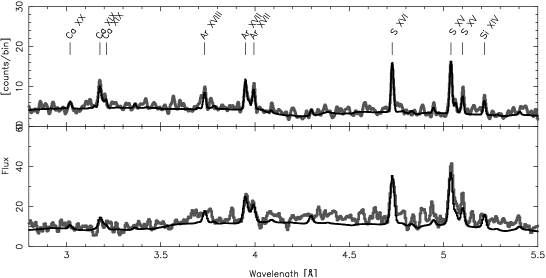
Figure 1: A portion of the IM Pegasi HETGS spectrum demonstrates the importance of resolution in line detection and measurement. The top panel shows the HEG spectrum, which has twice the resolving power of the MEG data (lower panel). Some emission lines, which are distinct in the HEG data, may not even appear as measurable features from the MEG. The smoother curve is a model, convolved with the instrumental response. The data are the sum of eight 25 ks exposures.

V Results for Active Binaries

The Solar corona is a common reference for interpretion of active binary spectra. Active binary stars are, however, three to four orders of magnitude more luminous in x-rays than the Sun. (Walter and Bowyer, 1981; Dempsey et al., 1993) It was not entirely surprising, then, when these stars showed very non-Solar characteristic coronal temperatures and abundances.

V.1 Elemental Abundances

High resolution spectroscopy has allowed more detailed evaluation of abundance anomalies first derived from low resolution data. (Singh et al., 1996; Huenemoerder et al., 2003) The Solar first ionization potential (FIP) effect (Feldman et al., 1990; Feldman, 1992; Feldman and Laming, 2000) is not followed. Instead, the trend is the reverse: high FIP elements are enhanced, though it is not a totally uniform or consistent trend. Examples may be found in Brinkman et al. (2001); Audard et al. (2001); Huenemoerder et al. (2001)

We have derived a preliminary set of abundances for IM Pegasi, for the same observations shown in Figure 1. They are rather typical results for coronally active binaries, with depleted Fe and enhanced Ne. Figure 2 shows the abundances relative to solar photospheric values versus the first ionization potential.

Figure 2: Abundances relative to Solar photospheric values for the IM Peg corona, as derived from the emission-measure and abundance fit to line fluxes. Uncertainties are the result of a Monte-Carlo iteration in which measured line fluxes were perturbed by their statistical measurement uncertainty. The $x$-axis is the first ionization potential.

The FIP is a convenient coordinate, but ultimately may not be physically significant. In the Sun, the coronal abundance drops by a factor of four at about 10 eV.Feldman and Laming (2000) Huenemoerder et al. (2003) compare the AR Lac results to Solar.

While we generally suspect that the abundance anomalies are important, we have no physical mechanism for predicting the fractionation, even in the Solar case. An additional complication we face with stellar coronae is that we often do not know the stellar photospheric abundances; they are difficult to determine from photospheric lines blended by rapid rotation.

The relative and absolute abundances must ultimately relate to the various mixing and segregating forces at work: gravitational settling, thermal diffusion, electrostatic forces, and bulk flows, for examples. In some cases, it appears that the relative abundances truly reflect an underlying physical phenomenon. As stars evolve, CNO processing occurs in the core, and can be dredged to the surface, and in binary systems, transferred to a companion in a dynamical mass-transfer phase. Drake (2003b); Drake and Sarna (2003) explore two scenarios with LETGS spectroscopy of C and N in a few stars and clearly show strong differences in the C and N line strengths in otherwise similar stars, consistent with stellar evolutionary theory.

V.2 Temperature Structure

As is obvious from Equation 1, temperature structure (the $DEM$) and abundances are not determined independently. They are highly degenerate if there is no coupling from element to element by overlapping emissivity functions. Fortunately, there are many ion states of iron present, typically from Fe xvii to Fe xxv. Many authors first derive the $DEM$ for Fe, then adjust abundances of other elements to bring the inferred emission measure into agreement with that of Fe. This is acceptable if the distributions strongly overlap. At the low end of the temperature range available to Chandra, however, there is little overlap of Fe with O or N, for example. In this case, we rely on the simultaneous fit to “bootstrap” N to O to Fe. A representative view of the HETGS line-temperature coverage can be found in Huenemoerder et al. (2003) (which also includes some ions from the extreme ultraviolet range).

We frequently find that the $DEM$ is double-peaked with components near $\log T\sim 6.8$ and $\sim 7.4$. (Huenemoerder et al., 2003; Drake et al., 2001) Weak, but significant, tails are seen on both the high and low sides. For the case of AR Lac, we had supplemental extreme ultraviolet data to extend the solution below $\log T=6.5$, and found that the minumum in the x-ray regime is real. On the hot end, the fit is poorly constrained since there are only a few weak lines with broad emissivity functions. The continuum also provides a high-temperature constraint, but also with low temperature resolution. That there is very hot material is undisputed, but the shape of the hot tail is not unique.

The solution to IM Pegasi (the same fit whose abundances are shown in Figure 2) is typical of active binaries and is shown in Figure 3.

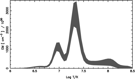
Figure 3: $DEM$ for IM Peg, from the same model in Figure 2. The width of the band is the standard deviation from the Monte-Carlo iteration.

We believe that the hotter peak is primarily due to flares, in analogy with impulsive magnetic reconnection events on the Sun which heat plasma. In the case of II Pegasi, we had enough data and a conveniently timed flare to model the $DEM$ in both pre-flare and flare states, and it was clear that the hot peak was due to the flare.(Huenemoerder et al., 2001) For AR Lac, with fewer flare counts, we relied on a proxy indicator: line flux modulation binned by temperature of formation, which showed that high $T$ lines — roughly coincident with the $DEM$ hotter peak — were highly modulated, but cooler lines were not.(Huenemoerder et al., 2003) Capella has only one peak near $\log T=6.8$, but does have a variable hot component which could be due to some lower level of flare contribution.Brickhouse et al. (2000)

V.3 Geometric Structure

The geometry of stellar coronae is of great interest. In the Sun, we have several different coronal structures: magnetically confined loops; open-field regions which merge the corona with the interplanetary medium; flaring loops; eruptive prominences; and bright points, to name a few. For other stars, we can only infer or indirectly image the surfaces and coronae. One method for determining scale is to search for rotational or eclipse modulation. Brickhouse et al. (2001) found modulation in 44 Boo, a short period eclipsing system, consistent with polar active regions on one component. In order to discriminate fluctuations due to flares, the high-resolution spectrum is necessary in order to exclude features formed predominantly at flare temperatures.

This effect is clearly demonstrated in a light curve of VW Cep, an 0.25 day period binary system. Figure 4 shows the count rate over 5 rotations in a short wavelength band (1.7–7 Å), the 17–25 Å region (which is dominated by iron and oxygen emission lines), and in the Ne x 12.3 Å line (which is blended with Fe xvii). It is obvious that the large flare is not seen in the low-temperature features. There is a hint that Ne x is systematically decreased near phase modulus 0.5; phase-folded curves will reveal whether we have detected compact coronal structure, or whether emission is uniformly distributed (or of large extent, relative to stellar radii).

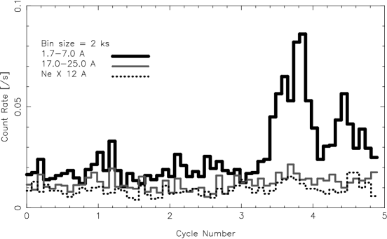
Figure 4: The counts in 2000 second bins vs. phase cycle are shown in 3 bandpasses for VW Cep, an 0.25 day period coronally active binary. The short-band curve (1.7–7 Å; upper, thick solid line) shows a sequence of large flares beginning near phase 3.5. The narrow bands (two lower curves; solid gray is 17–25 Å, and dotted is Ne x 12 Å), which are formed predominantly at lower temperatures than the short band, do not show the flares.

Radial velocity information can provide a general locus for coronal emission. Ayres et al. (2001) found that the Ne x centroid in HR 1099 followed the K1 IV star, indicating that it is the primary source of x-ray emission. Huenemoerder et al. (2003) used line width variability to determine that in AR Lac, both components were equal contributors to the x-ray flux.

VI Density Diagnostics

Young stars are well known as prodigious x-ray emitters,(Feigelson and Montmerle, 1999) and x-ray imaging is good for identifying young stars obscured by dust at optical wavelengths. The working hypothesis has been that since young stars are rapidly rotating, they have a strong magnetic dynamo, and they have activity analogous to that of the active binaries (which rotate rapidly due to their binary nature and tidal coupling).

Our first high resolution x-ray spectra of a classical T Tauri star (CTT; a youthful, low mass star, still actively undergoing accretion), TW Hydrae shed doubt on this interpretation.(Kastner et al., 2002) Neon is extremely overabundant, and iron very depleted, similar to, but more extreme than the typical coronal sources. Since we don’t yet know what fractionates the x-ray emitting plasma, this is still a curiosity without theoretical underpinning. The $DEM$ was very cool ($\log T\sim 6.5$) and narrow. This is different in general from active binaries, but not extreme, since it is not much different from Capella.

The single, starkly contrasting feature is in the ratios of the helium-like triplets: both Ne ix and O vii in TW Hya show ratios indicative of high density. Coupled with evidence from other wavelengths for accretion, Kastner et al. (2002) argued that the emission mechanism is not strictly “coronal” (magnetic loops and a dynamo), but somehow generated in an accretion funnel.

The sensitivity of the helium-like triplets to density has been known for a some time.(Gabriel and Jordan, 1969, 1973) The forbidden line is metastable; above some critical value, it can become depopulated by collisions, thereby reducing its flux in favor of the intercombination line. The ratio of the forbidden line ($f$) to the intercombination ($i$) is density sensitive above some critical density determined by the nuclear charge. In the Chandra bandpass, the most prominent He-like triplets are from Si xiii, Mg xi, Ne ix, O vii, N vi, and C v (the latter two are LETGS-only). These span a range of critical densities potentially useful for stellar plasma diagnostics. Ness et al. (2003) plot the critical densities of these ions. (There are other triplets present, such as S xv, Ar xvii, Ca xix, and Fe xxv, but the resolution is not sufficient to resolve them adequately.)

In order to pursue the nature of pre-main-sequence x-ray emission, we have recently obtained the HETGS spectrum of a weak-lined T Tauri (WTT) star, TV Crt (WTTs have presumably finished the accretion stage of evolution, but have not yet finished gravitational contraction to the main sequence when nuclear fusion starts and sustains pressure balance). We show its spectrum in Figure 5.

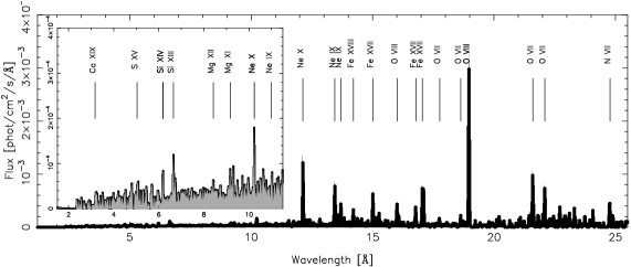
Figure 5: The Chandra HETGS spectrum of TV Crt (HD98800), a weak-lined T Tauri star. The inset shows an expanded view of the short wavelength region, with significant detections of features formed at high temperatures, and which are not present in the TW Hya spectrum.

The corona appears to be intermediate between TW Hya and the active binaries: it has a fairly cool component to the $DEM$, but also a warmer tail which drops off above $\log T\sim 7$.(Huenemoerder et al., 2004) To quantify the density diagnostic, we fit the $f/i$ ratio, and also the “G”-ratio, $(f+i)/r$ which is primarily sensitive to temperature ($r$ represents the resonance line flux). Figure 6 shows contours of confidence for these ratios for Ne ix ($\sim 13.6$ Å). The two stars are clearly distinct at the 99% confidence level.

Figure 6: We show the confidence countours for the Ne ix density ($R=f/i$) and temperature ($G=(f+i)/r$) sensitive line ratios for TW Hya and TV Crt, two pre-main sequence stars in the same physical association. Contours (inner to outer) are the 68, 90, and 99% limits. The small upper oval is for TW Hya, whose density is clearly constrained, and best fit value is about $\log n_{e}=12.5$. TV Crt (lower contours) only provides an upper limit of 12.25 (99% confidence). The grid overlay is from the density dependent atomic database, with $\log T$ labeled along the approximately horizontal direction, and $\log n_{e}$ vertically.

VI.1 A Warning

The positive density detection in TW Hya was easy, even in a rather low-signal observation, due to its extreme value. In other spectra, even deep observations, the measurement can be a very difficult task. Ness et al. (2003) present an in-depth study of Capella using HEG, MEG, LETG, and XMM-Newton grating spectra. They show that there is essentially no such thing as a model-independent line ratio. The only way to account for blends is to model the entire spectrum, then evaluate the relative contributions to any particular spectral feature using that model. They applied this to the Ne ix triplet, and found that about 30% of the intercombination line is due to iron. This 30% can change the $f/i$ ratio from an apparently constrained density measurement to unconstrained, even at HEG resolution.

VII Hot (High-Mass) Stars

At the other end of the temperature spectrum are the hot, high-mass main-sequence stars (O and B spectral types). The standard model for x-ray production in these objects was a massive, radiatively driven wind with shock instabilities.(Lucy and White, 1980) Temperatures were expected to be low. Due to outflow and optical depth effects, line profiles were expected to be blue-shifted and asymmetric. Chandra/HETGS spectra have changed that view. Some objects did behave as expected, such as $\zeta$ Puppis. (Kramer et al., 2003; Gagne et al., 2001; Cassinelli et al., 2001) Others did not: Schulz et al. (2003) found narrow, symmetric, and un-shifted lines in $\theta^{1}$ Ori C. It now appears that there can also be magnetically confined and very hot plasma in hot stars. There is currently a fairly large observational and theoretical campaign to explore and explain this unexpected behavior. Models of $\theta^{1}$ Ori C, which is periodically variable and has a measured magnetic field, have a wind channeled into a shock by primordial magnetic fields.(Gagne et al., 2001) It remains to be determined whether the previous x-ray/wind theory is the rule or the exception.