On the nature of eclipses in binary pulsar J0737-3039

Abstract

We consider magnetohydrodynamical interaction between relativistic pulsar wind and static magnetosphere in binary pulsar system PSR J0737-3039. We construct semi-analytical model describing the form of the interface separating the two pulsars. An assumption of vacuum dipole spin down for Pulsar B leads to eclipse duration ten times longer than observed. We discuss possible Pulsar B torque modification and magnetic field estimates due to the interaction with Pulsar A wind. Unless the orbital inclination is $\leq 86^{\circ}$, the duration of eclipses is typically shorter than the one implied by the size of the eclipsing region. We propose that eclipses occur due to synchrotron absorption by mildly relativistic particles in the shocked Pulsar A wind. The corresponding optical depth may be high enough if Pulsar A wind density is at the upper allowed limits. We derive jump conditions at oblique, relativistic, magnetohydrodynamical shocks and discuss the structure of the shocked Pulsar A wind. Finally, we speculate on a possible mechanism of orbital modulation of Pulsar B radio emission.

1 Introduction

A recent discovery of eclipsing binary pulsar system PSR J0737-3039 (Burgay et al. , 2003; Lyne et al. , 2004) may serve as an important tool in studying close environment of the neutron stars. In this system a fast recycled $P_{A}=22.7$ msec Pulsar A orbits a $P_{B}=2.77$ sec Pulsar B on a 2.4 hour orbit inclined at $\sim 87.7^{\circ}$ (with uncertanity of the order of unity) to the line of sight. Pulsar A shows $27$ sec frequency independent eclipses at the moments of superior conjunction (Kaspi et al. , 2004). In addition, Pulsar B shows orbital-phase dependent variations of intensity. It is also very weak at the inferior conjunction, consistent with being eclipsed as well (S. Ransom, private communication).

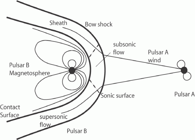
Figure 1: Cartoon of the binary pulsar system PSR J0737-3039. The wind of Pulsar A is shocked near Pulsar B and forms a sheath. Magnetosphere of Pulsar B is strongly distorted due to interaction with the wind. The system resembles the Earth-Solar wind interaction. On the ”day side” of Pulsar B magnetosphere (facing Pulsar A) the opening angle of the last closed field line may be much larger than in the case of isolated pulsar. In the sheath, the flow near the apex point is subsonic, while at larger angles it becomes supersonic both due to changing conditions at oblique shocks and due to pressure acceleration along the sheath. The contact surface is also expected to be unstable to Kelvin-Helmholtz instabilities.

In this paper we first construct a geometrical model of Pulsar A eclipses. Similarly to Arons et al. (private communication) we propose that the interaction of Pulsar A wind with Pulsar B magnetosphere resembles Solar wind – Earth magnetosphere interaction (see Fig 1). As a result, a bow shock forms in Pulsar A wind, separated from Pulsar B magnetosphere by a sheath of shocked material.

Absorption of Pulsar A radio emission may occur either in the shocked Pulsar A wind or in the magnetosphere of Pulsar B. If absorption occurs at cyclotron resonance with non-relativistic particles present on the closed field lines, then it is expected to be strongly frequency dependent, which is not observed. Synchrotron absorption by relativistic particles on the open field lines can give a frequency independent eclipse. Still, we disfavor this possibility, First, there are no indication of modulation of the eclipse by the rotation of Pulsar B (though the present temporal resolution may not be sufficient). Secondly, since the line of sight passes at the edge of magnetosphere (see Fig. 3), and since we see pulses from Pulsar B, it is hard to imagine geometry in which near the superior conjunction the line of light constantly passes through open field lines, giving full eclipses. Thirdly, the dimming of Pulsar B near the inferior conjunction is consistent with absorption being due to the shocked Pulsar A wind.

An alternative possibility for the location of the absorbing material, which we favor, is that the absorption occurs in the shocked Pulsar A wind, enveloping Pulsar B. Though the size of the shocked sheath is expected to vary by about $25\%$ due to Pulsar B rotation, it may still have an approximately constant column density and optical depth regardless of its size.

What determines the size of the eclipsing region? It may be determined either by geometric factors, so that the beginning and the end of the eclipse occur at the moment when the line of sight enters the absorbing region, or by microphysical processes in the plasma so that the eclipse occurs at the moment when optical depth $\tau$ to scattering/absorption becomes of the order of unity. We strongly prefer the geometrical interpretation of eclipses since any relevant microphysical process gives a frequency dependent absorption coefficient so that the condition $\tau\sim 1$ would occur at different points for different frequencies.

The geometrical (as opposed to microphysical) interpretation of the eclipse duration seems, at first sight, inconsistent with the data: a simple scaling of the size of Pulsar B magnetosphere would predict an eclipse which is much longer than observed. The light cylinder radius of Pulsar B is $1.29\times 10^{10}$ cm, so that its angular size seen from Pulsar A is $0.14$ rad. The line of sight passes $2.3^{\circ}=0.04$ rad $=3.6\times 10^{9}$ cm away from Pulsar B. Eclipsing part, corresponding to a 27 sec eclipse duration, is $1.8\times 10^{9}$ cm Kaspi et al.  (2004), which subtends a total angle of $0.02$ radians (see Fig. 2). Thus, the size of the eclipsing region is $\sim 0.04$ rad $=4\times 10^{9}$ cm, which is more than 3 times smaller than the light cylinder radius of Pulsar B.

A possible resolution of this disagreement is that the pressure of Pulsar A wind compresses Pulsar B magnetosphere to lateral sizes much smaller than the light cylinder. In this paper we first calculate semi-analytically the form of the interface between Pulsar A wind and Pulsar B magnetosphere. We find that if the magnetic field of Pulsar B is calculated using the vacuum dipole formula, the lateral size of the sheath is still much larger than the one inferred from eclipse duration. On the other hand, electromagnetic interaction of Pulsar B with the sheath strongly modifies the structure of the magnetosphere, so that the vacuum dipole formula becomes inapplicable. The modification of the spin down torque leads to an estimate of Pulsar B magnetic field which is typically 3-5 times smaller. Still, the size of the sheath is much larger than inferred from eclipse duration. A possible resolution is that inclination angle is $\leq 86^{\circ}$, so that the line of sight cuts at the edge of the sheath.

As independent parameters of the system we chose the spin down luminosities $L_{A}=5.8\times 10^{33}$ erg/sec and $L_{B}=1.6\times 10^{30}$ erg/sec and the separation of $D=9\times 10^{10}$ cm. These are the most reliable parameters, while the quantities like the inferred surface magnetic fields depend on the details of the magnetospheric structure.

2 Model of Pulsar A wind – Pulsar B magnetosphere interaction

Consider a point C on the interface between Pulsar A wind and Pulsar B magnetosphere defined by the radius-vector ${\bf r}_{B}(\theta_{B})$ (see Fig.  2). A normal to the interface makes an angle

$$\tan\alpha=\partial_{\theta_{B}}\ln r_{B}(\theta_{B})$$ (1)

with the radius-vector ${\bf r}_{B}(\theta_{B})$. Here $\theta_{B}$ is the polar angle between ${\bf r}_{B}$ and the normal to the plane of the orbit. At the same point, the radial flow from Pulsar A, leaving at the polar angle $\theta_{A}$, is inclined at angle $\phi$ to the interface. Angles $\alpha,\phi,\theta_{A}$ and $\theta_{B}$ are related by $\phi=\pi/2+\alpha-(\theta_{A}+\theta_{B})$. From the triangle $ABC$ we also find

$$\tan\theta_{A}+\tan\theta_{B}={D\over r_{B}\cos\theta_{B}}$$ (2)

and

$${r_{A}\over r_{B}}={\cos\theta_{B}\over\cos\theta_{A}}$$ (3)

We assume that the position of the interface is determined by the pressure balance between the static pressure of Pulsar B magnetic field and the dynamic pressure of Pulsar A wind (this is often called Newtonian approximation) :

$${L_{A}\sin^{2}\phi\over 4\pi r_{A}^{2}c}={\mu^{2}\over 8\pi r_{B}^{6}}f(\theta_{B})$$ (4)

where $\mu$ is the magnetic moment of the B pulsar and $f(\theta_{B})$ depends on the inclination of the magnetic moment. $f(\theta_{B})=1,~{}1+3\sin^{2}\theta_{B},~{}1+3\cos^{2}\theta_{B}$ for magnetic moments oriented along $x,y$ and $z$ correspondingly.

Next, we dimentionalize the problem by introducing $r_{B}\rightarrow rD$, $\xi=2L_{A}D^{4}/\mu^{2}$,

$${f(\theta_{B})\over r^{6}}={\xi\over 1+(\partial_{\theta_{B}}\ln r_{B}(\theta_{B}))^{2}}\left({r+\cos\theta_{B}\partial_{\theta_{B}}\ln r_{B}(\theta_{B})-\sin\theta_{B}\over 1-2r\sin\theta_{B}+r^{2}}\right)^{2},$$ (5)

which for a given $f(\theta_{B})$ is an ODE for $r(\theta_{B})$ depending on $\xi$ as a parameter. Next, instead of $\xi$ we introduce a dimensionless (measured in terms of $D$) stand-off distance $r_{0}$

$$\xi={(1-r_{0})^{2}\over r_{0}^{6}}f(\pi/2)$$ (6)

and parametrize $r\rightarrow r_{0}g(\theta)$. This gives

$${f(\theta_{B})\over f(\pi/2)}={g^{6}\over g^{2}+g^{\prime 2}}\left({(1-r_{0})(r_{0}g^{2}-g\sin\theta_{B}+g^{\prime}\cos\theta_{B})\over 1+r_{0}^{2}g^{2}-2r_{0}g\sin\theta_{B}}\right)^{2}$$ (7)

For a given stand-off distance $r_{0}$ Eq. (7) determines the form of the interface. We integrate this equation numerically, limiting integration to the regions close to Pulsar B light cylinder (near the apex point $g\sim 1+2(\pi/2-\theta_{B})^{2}/3$). Further down the stream the approximation of a static magnetosphere of Pulsar B breaks down and the balance at the contact discontinuity is determined by the pressure balance of two winds.

3 Magnetic field of Pulsar B

In order to find the stand-off distance we need to estimate a magnetic field strength of Pulsar B. This is not straightforward since the conventionally used vacuum dipole formula is not applicable in this case, as we argue below.

3.1 Vacuum dipole spindown

Conventionally, magnetic field of pulsars is determined by the vacuum dipole spin down formula

$$L={2\over 3}B_{NS}^{2}R_{NS}^{2}c\left({R_{NS}\Omega\over c}\right)^{4}$$ (8)

Even in case of isolated pulsars this is only an approximation since a large contribution to the torque comes from the currents flowing on the open field lines of magnetosphere.( If the typical current density is the Goldreich-Julian density times velocity of light, then the torque from the ${\bf j}\times{\bf B}$ force integrated over the open field lines gives the same estimate as the vacuum dipole luminosity (8).)

Equating (8) to the spin down luminosity $L_{B}=\Omega\dot{\Omega}I$, where $I\sim 10^{45}{\rm gcm^{2}}$ is the moment of inertial of neutron star, gives $B_{B}=1.5\times 10^{12}$ G (Lyne et al. , 2004). In this case $\xi=4\times 10^{7}$, $r_{0}=8.6\times 10^{-3}$ for $f(\pi/2)=1$ (when the B pulsar magnetic moment is oriented along $x$ or $z$ axis), and $r_{0}=1.07\times 10^{-2}$ for $f(\pi/2)=4$ (when the B pulsar magnetic moment is oriented along $y$ axis). The corresponding stand-off distances are $r_{m}=4.8\times 10^{9}$ cm and $r_{m}=6\times 10^{9}$ cm.

For these parameters $r_{0}$ we integrate Eq. (7). The results are given by upper set of curves in Fig 3. It is evident that the resulting size of the interaction sheath is much larger than the observed duration of the eclipse (the expected duration of the eclipse is $\sim 10$ times longer than observed).

3.2 Modification of the spindown of Pulsar B due to interaction with Pulsar A wind

Applicability of the vacuum spin down formula (8) in the case of interacting system PSR J0737-3039B is even more doubtful than in the case of isolated pulsars. Since the magnetospheric radius is located deep inside the light cylinder, the structure of Pulsar B magnetosphere is strongly distorted if compared with the vacuum case. The details of the structure are bound to be complicated.

Qualitatively, there are three possibilities for the structure of Pulsar B magnetosphere and corresponding spindown torque. (i) the interface may be a perfect conductor so that no Pulsar B field lines penetrate it. (ii) the interface may be a perfect resistor, so that all the Poynting flux from Pulsar B reaching it gets dissipated. (iii) the interface may be partially resistive so that large surface currents are generated, which together with the poloidal field of Pulsar B produce a torque on the star.

Modification of the spindown torque in all these cases are very different. We are mostly interested in cases (ii) and (iii). For case (ii), assuming that the typical current on the open field lines is of the order of the Goldreich-Julian current and that the size of the open field lines is determined by the magnetospheric radius $r_{m}$, the spin down becomes

$$L=\left({2\over 3}\right)B_{NS}^{2}r_{NS}^{2}c\left({\Omega r_{NS}\over c}\right)^{2}\left({r_{NS}\over r_{m}}\right)^{2}$$ (9)

Equating (11) to spin down luminosity $L_{B}$ and using the force balance (4), we find

$$B_{B}={3^{3/4}\over 2}{\sqrt{D}L_{B}^{3/4}\over L_{A}^{1/4}r_{NS}^{3}\Omega^{3/2}}=4.7\times 10^{11}\,{\rm G}\mbox{}$$

$$r_{m}={3^{1/4}\over\sqrt{2}}\left({L_{B}\over L_{A}}\right)^{1/4}\sqrt{{cD\over\Omega}}=4\times 10^{9}\,{\rm cm}$$ (10)

Using parameters (10) we integrate Eq. (7) (the middle solid curve on Fig. 3; in this case $r_{0}=0.045$ for $\mu=\mu_{x}$). The size of the sheath is only slightly modified if compared with the vacuum dipole and is much larger than the one implied by eclipse duration.

Finally, the interface may be partially resistive. Relativistic boundary layers are strongly unstable on scales of tens to hundreds of gyroradii (Smolsky & Usov, 1996; Liang et al. , 2003), so that for ultra-relativistic electrons with $\gamma\sim 10^{6}$ the kinetic thickness of the interface may become macroscopically large. As a result, Pulsar B field may penetrate the interface, similar to what may happen in neutron star – disk interaction (e.g.  Ghosh &Lamb, 1979a, b; Wang, 1995). In this case the poloidal magnetic field of Pulsar B will be twisted by the pulsar rotation to produce toroidal magnetic field which may be as high as poloidal magnetic field at the interface, $B_{\phi}(r_{m})\leq B_{B}(r_{m})$. (Since the magnetospheric radius is much smaller than the light cylinder radius, light travel effects may be neglected.) The resulting surface current on the interface together with the poloidal field will produce a ${\bf j}\times{\bf B}$ force and a torque on the pulsar. The spin down then becomes

$$L=\left({1\over 2}\right)\left({2\over 3}\right)B_{NS}^{2}r_{NS}^{2}c\left({r_{NS}\over r_{m}}\right)^{3}\left({\Omega r_{NS}\over c}\right)$$ (11)

A factor $1/2$ has been introduced in front to account for the fact that only the part of pulsar B magnetosphere facing Pulsar A experiences the torque.

Equating (11) to spin down luminosity $L_{B}$ and using the force balance (4), we find

$$B_{B}={3\over\sqrt{2}}{DL_{B}\sqrt{c}\over\sqrt{L_{A}}r_{ns}^{3}\Omega}=3\times 10^{11}~{}{\rm G}\mbox{}$$

$$r_{m}=\left({3\over 2}\right)^{1/3}\left({L_{B}\over L_{A}}\right)^{1/3}\left({cD^{2}\over\Omega}\right)^{1/3}=3.5\times 10^{9}{\rm cm}$$ (12)

Magnetic field in this case is $\sim 5$ times smaller.

Using parameters (12) we integrate Eq. (7) (the lower solid curve on Fig. 3; in this case $r_{0}=0.038$ for $\mu=\mu_{x}$).

Both modified magnetic field estimates (10-12) predict the size of pulsar B magnetosphere which is 2-3 times larger than inferred by eclipse duration. A possible resultion of the disagreement is that the orbital inclination angle is $\leq 86^{\circ}$.

3.3 Spin down due to propeller effect and Magnus force on Pulsar B

Interaction of Pulsar B with the wind of Pulsar A may also produce propeller effect, whereby the material of Pulsar A wind is flung off by the rotation of Pulsar B. As a result, there will be extra torque on Pulsar B produced by the Magnus force (a force due to a difference in pressures at the two sides of the Pulsar B magnetosphere with rotation velocity aligned and counter-aligned with the radial wind of Pulsar A, c.f. a ”dry leaf” kick in soccer). Next we estimate the importance of the propeller effect on the spin down of Pulsar B.

The torque of the Magnus force acting on Pulsar B can be estimated as

$$T={L_{A}\Omega^{2}r_{m}^{5}\over 4D^{2}c^{3}}$$ (13)

Equating this to the change of angular momentum we find the corresponding magnetospheric radius

$$r_{m}=2^{2/5}\left({L_{B}\over L_{A}}\right)^{1/5}\left({c^{3}D^{2}\over\Omega^{3}}\right)^{1/5}=7.2\times 10^{9}{\rm cm}$$ (14)

This radius is larger than the one given by the dipole formula. Thus, we conclude that the propeller effect is not important for the spin evolution of Pulsar B.

4 Eclipsing mechanism: synchrotron absorption

We propose that the absorption of Pulsar A radio beam occurs due to the synchrotron absorption in the shocked plasma. We parametrize Pulsar A wind by a magnetization parameter $\sigma$, the ratio of Poynting to particle fluxes (Kennel & Coroniti, 1984a). The magnetic field in the sheath (in the laboratory frame) is

$$B=3\sqrt{{\sigma\over 1+\sigma}}\sqrt{2L\over cD^{2}}=21\sqrt{{\sigma\over 1+\sigma}}\,{\rm G}=1.2\,{\rm G}$$ (15)

where the last equality assumes $\sigma=3\times 10^{-3}$, a value inferred for Crab pulsar (Kennel & Coroniti, 1984a). The factor of 3 in front assumes a compression in strong relativistic fluid shock (see also Section 5 for more details). The non-relativistic cyclotron frequency inside the sheath is $\nu_{B}=2.4$ MHz. In order to absorb at the observed frequencies $\nu_{obs}\sim 1$ GHz, the particles should be relativistic with a Lorentz factor $\gamma\sim\sqrt{\nu_{obs}/\nu_{B}}=30$. It is not obvious at all that such particles are present in the shocked flow. Estimates of the bulk Lorentz factor in case of the Crab pulsar give $\Gamma\sim 10^{6}$ (Kennel & Coroniti, 1984b). If a similarly high Lorentz factor is assumed for PSR J0737-3039A, then one expects that the lowest energy cut-off in the shocked flow is similarly high, $\gamma\sim\Gamma$.

On the other hand, radio emission of the Crab nebula is attributed to electrons with much lower energies, $\gamma\ll\Gamma$. These electrons may be either cooled remnants of the intense early injection Atoyan (1999), or, more likely, may represent a completely different population of accelerated particles. Thus, invoking the Crab pulsar as an example, it is feasible that relativistic magnetized shocks do produce a low energy population of electrons. Note, though, that since the magnetic fields in the bulk of the Crab nebular and in the sheath of the interacting winds of PSR J0737-3039 differ by some 4 orders of magnitude, the corresponding Lorentz factors of synchrotron emitting/absorbing particles differ by two orders of magnitude. Unfortunately, in the absence of understanding of the acceleration mechanism of radio electrons we cannot judge whether this is possible. (Alternatively, it is feasible that the low energy population in the sheath comes from Pulsar B due to a ”leakage” through the interface.)

Below we assume that a population of low energy electrons with a power law distribution $n(\epsilon)=\kappa\epsilon^{-p}$ is indeed present in the sheath ($\epsilon$ is the energy of particles). The parameter $\kappa$ is related to the density of pairs and the low and high energy cut-offs in the spectrum, $\kappa\sim nmc^{2}/(p-1)\gamma_{min}^{p-1}\sim nmc^{2}$ where we assumed that $\gamma_{min}\sim 1$ and $p$ close to 2.

Cyclotron absorption coefficient is then (Lang, 1974)

$$\alpha_{\nu}^{0}=2\times 10^{-2}\,g(p)\,(3.5\times 10^{9})^{p}\,\kappa\,B^{(p+2)/2}\,\nu^{-(p+4)/2}\,{\rm cm^{-1}}$$ (16)

where $g(p)$ is a coefficient of the order of unity, $\nu$ is observing frequency. We also assumed that radiation propagates orthogonally to the field lines.

We normalize the pair density in the wind to the Goldreich-Julian density at Pulsar A light cylinder. The particle flux for the Pulsar A is then $\dot{N}_{A}=\lambda\sqrt{4\pi L_{A}c/e^{2}}\sim\lambda\times 10^{32}s^{-1}$ and the density at distance of Pulsar B is $n_{A}=\dot{N}_{A}/(4\pi cD^{2})=3\times 10^{-2}\lambda$ cc. In order to estimate the thickness and the particle density in the sheath it is necessary to know the details of the flow structure. As a simple estimate we assume that the column density through the sheath is of the order of the column density of Pulsar A at the distance of Pulsar B, $\sim n_{A}D$. For particle index $p=2$ we find

$$\tau_{0}\sim 3\times 10^{-6}\lambda\left({\nu\over 1GHz}\right)^{-3}$$ (17)

Thus, in order to produce optical depth $\geq 1$ the multiplicity factor should not be quite large $\lambda\geq 10^{6}$ (flatter spectra $p\leq 2$ give higher optical depth also, for $p=1.5$ it increases by an order of magnitude). The required multiplicity is large, but not impossible (a value of multiplicity factor invoked for the Crab is $\lambda=10^{6}$, (Kennel & Coroniti, 1984a), see also Arons & Scharlemann (1979); Muslimov & Harding (2003)).

We conclude that synchrotron absorption by weakly relativistic particles in the shocked Pulsar A wind is a possible eclipsing mechanism, but acknowledge that the required wind multiplicity is at the upper possible end.

5 Dynamics of the shocked Pulsar A wind

In the previous section we calculated semi-analytically the form of the interface between Pulsar A wind and Pulsar B magnetosphere. In reality, the interface will consist of the bow shock and a contact discontinuity (see Fig 1). In this section we study the dynamics of the shocked pulsar wind in the sheath. We first derive the oblique jump conditions for relativistic MHD shocks. Relativistic oblique fluid shocks have been considered by Konigl (1980); we are not aware of a work which considered relativistic oblique MHD shocks. We apply the results to PSR J0737-3039, assuming that the form of the shock follows the form of the interface calculated in Sections 2 and 3.

5.1 Oblique fluid shocks

Let the stream lines make an angle $\phi$ with the shock and let the post-shock flow make an angle $\chi$ with the initial velocity (Fig. 5). Oblique shock conditions can be obtained from normal shocks and an additional condition that the component along the shock velocity remains constant.

$$n_{1}u_{1}\sin\phi=n_{2}u_{2}\sin(\chi-\phi)\mbox{}$$

$$w_{1}u_{1}^{2}\sin^{2}\phi+p_{1}=w_{2}u_{2}^{2}\sin^{2}(\chi-\phi)+p_{2}\mbox{}$$

$$w_{1}\gamma_{1}u_{1}\sin\phi=w_{2}\gamma_{2}u_{2}\sin(\chi-\phi)\mbox{}$$

$${u_{1}^{2}\cos^{2}\phi\over 1+u_{1}^{2}\sin^{2}\phi}={u_{2}^{2}\cos^{2}(\phi-\chi)\over 1+u_{2}\sin^{2}(\phi-\chi)}$$ (18)

where $w$ is enthalpy, $u$ is four-velocity, $n$ is density, $p$- pressure and $\gamma$ is Lorentz factor; velocity of light has been set to unity. Subscripts denote unshocked (1) and shocked (2) fluids. Relations (18) can be resolved (Landau & Lifshitz, 1975)

$$u_{1}\sin\phi=\sqrt{(e_{2}+p_{1})(p_{2}-p_{1})\over(e_{1}+p_{1})(e_{2}-e_{1}-(p_{2}-p_{1})}\mbox{}$$

$$u_{2}\sin(\chi-\phi)=\sqrt{(e_{1}+p_{2})(p_{1}-p_{2})\over(e_{2}+p_{2})(e_{1}-e_{2}-(p_{1}-p_{2})}\mbox{}$$

$${n_{1}\over n_{2}}={u_{2}\sin(\chi-\phi)\over u_{1}\sin\phi}=\sqrt{(e_{1}+p_{2})(e_{1}+p_{1})\over(e_{2}+p_{1})(e_{2}+p_{2})}\equiv\eta$$ (19)

where $w=e+p$ and $\eta$ is the compression ratio, defined here as a ratio of rest frame densities.

For adiabatic flow, using relations

$$w=n+{\Gamma_{a}\over\Gamma_{a}-1}p={u_{s}^{2}+1\over u_{s}^{2}}p\Gamma_{a}$$ (20)

where $u_{s}$ is a sound four-velocity, and $\Gamma_{a}$ is adiabatic index. The compression ratio $\eta$ can be expressed as a function of $u_{s,1}$ and $u_{s,2}$. The corresponding relations are too bulky to be reproduced here. In the case of initially cold plasma ($p_{1}=0$, $w_{1}=e_{1}=n_{1}$, $u_{s,1}=0$) we find

$$u_{1}^{2}={(\Gamma_{a}-1)(\Gamma_{a}(1-\eta)-(1+\eta))\over\Gamma_{a}(2-\Gamma_{a}(1-\eta))\eta^{2}\sin^{2}\phi}\mbox{}$$

$$u_{2}=\eta u_{1}{\sin\phi\over\sin(\chi-\phi)}\mbox{}$$

$$u_{s,2}^{2}={(\Gamma_{a}-1)(\Gamma_{a}(1-\eta)-(1+\eta))\over\Gamma_{a}(3-\eta)-\Gamma_{a}^{2}(1-\eta)-2-\eta}$$ (21)

In the non-relativistic limit $u\ll 1$ these relations give $\eta=(\Gamma_{a}-1)/(\Gamma_{a}+1)+{{\cal{O}}(u^{2})}$, while in the strongly relativistic limit $u_{1}\gg 1$, $\eta\ll 1$,

$$\eta={\Gamma_{a}-1\over u_{1}\sin\phi\sqrt{\Gamma_{a}(2-\Gamma_{a})}}={1\over 2\sqrt{2}u_{1}\sin\phi}\mbox{}$$

$$u_{2}={\Gamma_{a}-1\over\sqrt{\Gamma_{a}(2-\Gamma_{a})}}={1\over 2\sqrt{2}}{\sin\phi\over\sin(\chi-\phi)}\mbox{}$$

$$u_{2,s}=\sqrt{\Gamma_{a}-1\over 2-\Gamma_{a}}={1\over\sqrt{2}}$$ (22)

where the second equalities assume $\Gamma_{a}=4/3$ (this is also assumed for all numerical estimates below). Thus, for cold flow $0<\eta<(\Gamma_{a}-1)/(\Gamma_{a}+1)$.

As independent parameters of the problem we chose the initial four-velocity $u_{1}$ and the compression ratio $\eta$. For a particular case of cold plasma $u_{1}$ and $\eta$ are related by Eq. (21).

Eliminating $u_{2}$ from Eqns. (18), we can determine $\chi(\phi,u_{1})$:

$$\tan^{2}(\phi-\chi)=\eta^{2}{1+u_{1}^{2}\sin^{2}\phi\over 1+\eta^{2}u_{1}^{2}\sin^{2}\phi}\tan^{2}\phi$$ (23)

which, using Eq. (21) gives

$$\tan\chi={\Gamma_{a}(1-\eta)\tan\phi\over 1+(1-\Gamma_{a}(1-\eta))\tan^{2}\phi}$$ (24)

For strong shocks, $\eta\rightarrow 0$,

$$\tan\chi={\Gamma_{a}\tan\phi\over 1-(\Gamma_{a}-1)\tan^{2}\phi}$$ (25)

For $\Gamma_{a}=4/3$, the maximum deflection angle $\chi_{max}=\pi/6$ is reached at $\phi_{max}=\pi/3$.

We can also determine the post-shock Mach number:

$$M_{2}^{2}={u_{2}^{2}\over u_{2,s}^{2}}={u_{1}^{2}\over u_{2,s}^{2}}{\cos^{2}\phi+(1+u_{1}^{2})\eta^{2}\sin^{2}\phi\over 1+u_{1}^{2}\sin^{2}\phi}\approx{2\cos^{2}\phi+1/4\over\sin^{2}\phi}$$ (26)

For initially cold flow, the compression ratio $\eta$ can be eliminated using relations (21); then Eq. (26) can be solved for the angle $\phi_{M}$ at which the post shock flow is sonic. We find $\phi_{M}=\phi_{max}=\pi/3$.

5.2 Oblique MHD shocks

Next we find jump conditions for strong, ultra-relativistic fast magnetosonic shocks, assuming that the magnetic field lies in the plane of the shock. (When the field is in the plane of the shock, the relevant MHD expressions can be obtainable by generalizing the hydrodynamical relations by substituting for the pressure $p$ and internal energy density $\epsilon$: $p\rightarrow p+b^{2}/8\pi$, $\epsilon\rightarrow\epsilon+b^{2}/8\pi$.) The shock jump conditions for relativistic MHD shocks are Landau & Lifshitz (1975)

$$b_{1}u_{1}\sin\phi=b_{2}u_{2}\sin(\chi-\phi)\mbox{}$$

$$\left(w_{1}+b_{1}^{2}\right)u_{1}^{2}\sin^{2}\phi+p_{1}+{b_{1}^{2}\over 2}=\left(w_{2}+b_{2}^{2}\right)u_{2}^{2}\sin^{2}(\chi-\phi)+p_{2}+{b_{2}^{2}\over 2}\mbox{}$$

$$\left(w_{1}+b_{1}^{2}\right)u_{1}\sin\phi\gamma_{1}=\left(w_{2}+b_{2}^{2}\right)u_{2}\sin(\chi-\phi)\gamma_{2}$$ (27)

(continuity equation and equation for velocity along the shock remain the same). In Eq. (27) $b$ is a rest frame magnetic field times $\sqrt{4\pi}$. Equations (27) can be resolved

$$u_{1}=\sqrt{\left((b_{1}^{2}-b_{2}^{2})/2+p1-p_{2}\right)\left((b_{1}^{2}+b_{2}^{2})/2+p1-p_{2}+w_{2}\right)\over 2(b_{1}^{2}+w1)(2(p_{2}-p_{1})+w2-w1)}{1\over\sin\phi}\mbox{}$$

$$u_{2}=\eta{\sin\phi\over\sin(\phi-\chi)}u_{1}\mbox{}$$

$$\eta={n_{1}\over n_{2}}={b_{1}\over b_{2}}={u_{2}\sin(\phi-\chi)\over u_{1}\sin\phi}=\sqrt{\left(w_{1}+b_{1}^{2}\right)\left(w_{1}-p_{1}+p_{2}+(b_{1}^{2}+b_{2}^{2})/2\right)\over\left(w_{2}+b_{2}^{2}\right)\left(w_{2}-p_{2}+p_{1}+(b_{1}^{2}+b_{2}^{2})/2\right)}$$ (28)

To characterize the magnetization of the flow we introduce parameter (see Kennel & Coroniti (1984a))

$$\sigma={b_{1}^{2}\over w_{1}}$$ (29)

which is the ratio of the rest frame magnetic and plasma energy densities (it is also equal to the ratio of Poynting to particle fluxes).

Similarly to the fluid case, the compression ratio (28) can be written in terms of preshock and post-shock fast magnetosonic four-velocities

$$u_{s}^{2}={p\Gamma_{a}+w\sigma\over w-p\Gamma_{a}}$$ (30)

If the preshock plasma is cold and in the limit of strong shocks $\eta\rightarrow 0$ (it is also necessary that $u_{1}^{2}\gg\sqrt{\sigma}$), and assuming $\Gamma_{a}=4/3$, we find

$$u_{1}={1\over\eta}\sqrt{{2+\Gamma_{a}(\sigma-2)-4\sigma-\sqrt{\Gamma_{a}^{2}(2+\sigma)^{2}+4(1+2\sigma)^{2}-4\Gamma_{a}(2+3\sigma+2\sigma^{2})}\over 8(2-\Gamma_{a})\left(\sqrt{\Gamma_{a}^{2}(2+\sigma)^{2}+4(1+2\sigma)^{2}-4\Gamma_{a}(2+3\sigma+2\sigma^{2})}+2+(4-\Gamma_{a})\sigma\right)}}=\mbox{}$$

$${1+4\sigma+\sqrt{1+16\sigma(\sigma+1)}\over 2\sqrt{2}\eta\sqrt{3+4\sigma+\sqrt{1+16\sigma(\sigma+1)}}}\equiv{f(\sigma)\over\sin\phi\eta}\mbox{}$$

$$u_{2,s}=\sqrt{\Gamma_{a}-1+\sigma\over 2-\Gamma_{a}}=\sqrt{1+3\sigma\over 2}$$ (31)

(cf. Kennel & Coroniti (1984a)). Equation (31) defines the function $f(\sigma)$.

Equations describing oblique relativistic MHD shocks remain the same as in the fluid case, with dependence $u_{1}(\eta)$ given by (31). The deflection angle becomes

$$\tan\chi={(f(\sigma)+\sqrt{1+f(\sigma)^{2}})\tan\phi\over\sqrt{1+f(\sigma)^{2}}-f(\sigma)\tan^{2}\phi}$$ (32)

The maximum deflection angle is reached

$$\cos\phi_{max}=\sqrt{f(\sigma)(\sqrt{1+f(\sigma)^{2}}-f(\sigma))}$$ (33)

As $\sigma\rightarrow\infty$, $\phi_{max}\rightarrow\pi/4$, $\chi_{max}\rightarrow 1/(4\sigma)$.

Similarly to the hydrodynamic case, using Eq. (26), we can find the angle $\phi_{1}$ at which the post shocked flow remains sonic. In the ultra-relativistic limit we find

$$\sin\phi_{M}=\sqrt{(2-\Gamma_{a})(1+f(\sigma)^{2})\over 1+\sigma}$$ (34)

(see Fig. 7). As $\sigma\rightarrow\infty$, $\phi_{M}\rightarrow\arcsin\sqrt{2\over 3}=54.73^{\circ}$, $\chi_{M}\rightarrow 1/(3\sqrt{2}\sigma)$.

Using the relations derived in the previous section we can calculate the post shock velocities (Fig. 8). At larger angles the post-shock flow becomes relativistic, $\Gamma_{s}\geq 1$ ($\Gamma_{s}$ is the post-shock Lorentz factor).

6 Pulsar B emission

Another puzzling property of PSR J0737-3039 is the variations of Pulsar B flux depending on the orbital phase (Lyne et al. , 2004). In addition to two sections of the orbit where it is very bright, so that single pulses can be seen, the flux density of the pulsar B emission is at a minimum near, but centered slightly before, the inferior conjunction. It is not clear if the flux goes to zero (Ransom, private communication). One possibility is that Pulsar A wind leaks through the interface and affects the microphysical process responsible for the generation of radio emission by Pulsar B, somewhat similar to the so-called flux transfer events at the day side of Earth magnetosphere (Fahr et al. , 1986). Such process is prohibited in ideal MHD and should occur through resistive effects (e.g. tearing mode). The fact that the magnetized boundary becomes “leaky” and both plasma and magnetic field are transported across it, has been amply demonstrated through decades of space experiments (e.g.  Cowley, 1982). The transport occurs either due to microscopic resistive instabilities of the surface current (Galeev et al. , 1986) or due to dynamic (e.g. RT) instabilities.

Can Pulsar A affect Pulsar B electrodynamics? We have previously estimated the density of Pulsar A wind at Pulsar B to be $n_{A}\sim 3\times 10^{-2}\lambda$ cc. For Pulsar B, the particle flux is $\dot{N}=\lambda\sqrt{4\pi cL_{B}/e^{2}}=10^{30}\lambda s^{-1}$ (surface Goldreich-Julian density $n_{GJ,surf,B}=2.2\times 10^{9}cm^{-3}$), so that the density at the interface $r_{m}\sim 2\times 10^{9}$ cm is $n_{B}\sim 0.27\lambda$ cc. Thus, if the multiplicity factors are equal for both pulsars, the particle density of Pulsar B flow on the open field lines is two orders of magnitude larger than the density of Pulsar A wind. Overall, Pulsar A wind can make only a small contribution to the particle density in Pulsar B magnetosphere. On the other hand, the assumption of equal multiplicity factors may not hold in the gaps of Pulsar B - regions of low density, where $\lambda_{B}\sim 1$. If Pulsar A plasma can get onto field lines passing through Pulsar B gaps, and if $\lambda_{A}\geq 100$, this can strongly affect particle acceleration in Pulsar B gaps and radio emission generation.

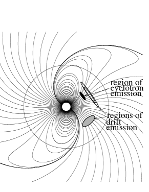
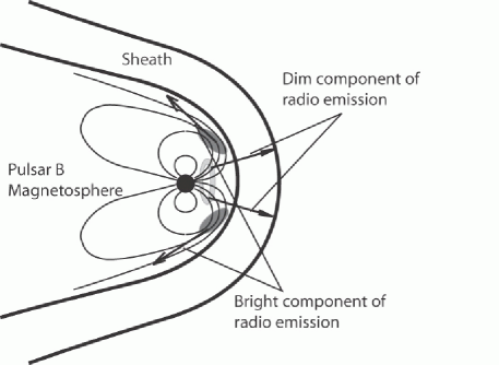
Figure 9: (a) Fig. 5 from Lyutikov et al.  (1999a) showing the location of radio emission generation regions in isolated pulsars (field structure is that of a vacuum rotating dipole). ”The location of the Cherenkov-drift emission depends sensitively on the curvature of magnetic field line. Two possible locations of the Cherenkov-drift emission are shown: ringlike near the magnetic axis and in the region of swept field lines.” (b) Possible modification due to interaction with Pulsar A wind. The dim component of emission is not affected by the Pulsar A wind and is produced at all phases of Pulsar B rotation, while the bright component is produced only at the side of Pulsar B magnetosphere facing Pulsar A.

Finally, we suggest a possible explanation for sudden increases in brightness of Pulsar B at two particular sections in the orbit. The dynamical compression of Pulsar A wind may change the condition for radio emission generation if generation takes places at large distances from the pulsar, as has been suggested by Lyutikov et al.  (1999a) (see also Kazbegi et al.  (1991) For example, the growth rate of Cherenkov-drift instability (Lyutikov et al. , 1999b) depends sensitively on the radius of curvature of magnetic field lines. Due to strong pressure from Pulsar A wind, the open field lines of Pulsar B are much stronger curved, than in isolated pulsars, producing larger growth rates (growth rates for Cherenkov-drift instability are marginal in isolated pulsars, (Lyutikov et al. , 1999b)). Cherenkov-drift instability develops at a limited range of radii and produces emission which is beamed along the local magnetic field. As Lyutikov et al.  (1999a) have argued, emission is produced at two locations: in a ring-like region near the magnetic axis and in the region of swept back magnetic field lines. In the latter case the radio emission is produced at large angles with respect to the magnetic axis (see Fig. 9). We propose that the transient brightening of Pulsar B occurs when the line of sight runs parallel to the magnetic field lines in the emission generation region located on the bend-back field lines, close to the edge of Pulsar B magnetosphere.

The immediate implication of the model is that the pulse profile of Pulsar B should change with the orbital phase, as the new emission region comes into line of sight at particular parts of the orbit. Preliminary data indicate that this is indeed the case (S. Ransom, private communication).

An important prediction of the Cherenkov-drift instability, which is in stark contrast to the the bunching theory of radio emission, is that the emitted waves are polarized perpendicular to the plane of the curved magnetic field line. Thus at the swept-back field lines polarization is along the axis of rotation. This may be used as a test to distinguish between the two theories. Assuming that Pulsar B is an orthogonal rotator with the rotational axis along the normal to the orbital plane, the Cherenkov-drift emission will be linearly polarized along the normal to the orbit as well.

7 Discussion

In this paper we considered magnetohydrodynamic interaction between relativistic pulsar wind and static magnetosphere in double pulsar system PSR J0737-3039. Our main conclusion are:

• Electromagnetic torque on Pulsar B is increased due to the interaction with Pulsar A wind. Depending on the nature of interaction, the magnetic field of Pulsar B can be as low as $3\times 10^{11}$ G. Still, the geometrical model for the form of the interface predicts the size of the interface which is much larger than inferred from the duration of Pulsar A eclipses, unless the orbital inclination angle is $\leq 86^{\circ}$.

• A likely cause of eclipses is synchrotron absorption in the dense shocked Pulsar A wind by low energy relativistic electrons. The density of Pulsar A wind should be at the upper allowed limit. The presence of such electrons cannot be justified from first principles.

The major uncertainty of the model is the source of low energy, $\gamma\sim 30$, electrons in the sheath. Pulsar A wind cannot be so slow: otherwise induced Compton scattering in the wind will make it unobservable (Sincell & Krolik, 1992). One possibility is that such low energy electrons are accelerate not at the shock, but at the rotational discontinuity during development of dynamic and/or resistive instabilities. Alternatively, mixing of Pulsar A and Pulsar B plasmas, initiated by such instabilities, may populate the sheath with weakly relativistic electrons accelerated in Pulsar B gaps. If mixing is efficient, particle number density in the sheath may be dominated by Pulsar B plasmas. Yet another possibility is that absorption happens on the strongly bend-back open field lines of Pulsar B which asymptotically take the form of the sheath (it would be hard to distinguish this possibility from absorption in the sheath itself).

Our calculations are consistent with the possibility that Pulsar A wind experiences a strong shock near Pulsar B. This limits the magnetization parameter to $\sigma\leq\Gamma^{2}$ (this is a condition that the preshock Lorentz factor $\Gamma$ is larger than the Alfvén speed in the wind). Thus, our results do not necessarily imply that Pulsar A wind is kinetically dominated near Pulsar B. (The energy required to create a population of low energy electrons is a $1/\sigma$ fraction of the total wind energy; this is also a fraction of energy dissipated in a strongly magnetized shock with $\sigma\gg 1$, (Kennel & Coroniti, 1984a).)

A possible measurement of $\sigma$ may come from high energy observations of the system. Shocks in kinetically dominated winds are expected to be strongly dissipative so that a large fraction of the incoming energy flux may be radiated in X-rays. The expected luminosity is $L_{X}\sim L_{A}\Delta\Omega\sim 3\times 10^{30}$ erg/sec, where $\Delta\Omega\sim 5\times 10^{-3}$ is the solid angle of the shocked region seen from Pulsar A. A recent detection of a weak X-ray emission (McLaughlin et al. , 2004) at a level $2\times 10^{30}$ erg/sec is consistent with this scenario. (A confirmation of this result is needed since the count rate was too low and the X-ray emission is also consistent with Pulsar A magnetospheric emission.)

A better understanding of the system should come from the full relativistic MHD modeling of the system. The relations for oblique relativistic MHD shocks derived in this paper can be used as guidelines and a check to such simulations. Qualitatively, the flow in the sheath is expected to become supersonic both due to the changing shock conditions and due to pressure acceleration away from the apex point, so that the flow will form a de Laval nozzle. In addition, centrifugal forces acting on a flow moving along the curved trajectory (so called Busemann correction) need to be taken into account. Another important property of the shocked flow is that even for small magnetization of Pulsar A wind $\sigma\ll 1$ magnetic field plays an important role near the contact discontinuity and cannot be neglected. Thus, any credible simulation of the interaction must use full relativistic MHD formalism.

Figure 2: Geometry of the interaction. Pulsar A is located at distance $D$ from Pulsar B along the $y$ axis. Magnetic moment of Pulsar B may be oriented along any of the axis $x,y,z$. Pulsar A wind is shocked near Pulsar B. At point C on the interface surface, defined by ${\bf r}_{B}(\theta_{B})$, the surface normal makes an angle $\alpha$ with ${\bf r}_{B}$. At the same point, the radial flow from Pulsar A is inclined at angle $\phi$ to the surface. The insert shows the eclipsing region (in radians) as viewed from Pulsar A.

Figure 3: Form of the contact surface in the $y-z$ plane for different orientations of Pulsar B magnetic dipole. Pulsar B is located at the origin, Pulsar A is located at $y=1$. Upper curves for magnetic field of Pulsar B assuming standard spin down luminosity ($B_{B}=1.5\times 10^{12}$ G). Solid lines are for $\mu=\mu_{x}$ (in the plane of orbit along the Pulsar B orbital velocity), dashed lines are for $\mu=\mu_{y}$ (along the line connecting the two pulsars) and dotted lines for $\mu=\mu_{z}$ ( perpendicular to the orbital plane; observationally, large $\mu_{z}$ is excluded since we do see the pulses from Pulsar B). Asymptotic opening angle is $\sim 0.11-0.13$ rad. Lower solid curves for magnetic field of Pulsar B with modified torques $B_{B}=4.7\times 10^{11}$ (Eq. 10) (asymptotic opening angle is $\sim 0.09$ rad) and $B_{B}=3\times 10^{11}$ G (Eq. 12) (asymptotic opening angle is $\sim 0.07$ rad). Long dashed line is the line of sight (inclination $87.7^{\circ}$). Dash-dot line is the light cylinder radius (it looks non spherical due to different axial scales).

Figure 4: Angle of attack $\phi$ as a function of polar angle. Negative $\theta_{B}$ refer to parts of the interface facing Pulsar A. Labeling of the curves is the same as in Fig. (3).

Figure 5: Geometry of oblique shock flow.

Figure 6: Dependence of the deflection angle $\chi$ on the angle of attack $\phi$ for initially cold ($p_{1}=0$) fluid for different $u_{1}$ and $\Gamma=4/3$. $u_{1}\rightarrow 0$ corresponds to non-relativistic case.

Figure 7: Dependence of the deflection angle $\chi$ on the angle of attack $\phi$ for ultra-relativistic MHD shocks $u_{1}\gg 1$ and different magnetization parameters $\sigma$. Dotted lines gives the maximum deflection angle (Eq. (33)), dashed line demarcates the subsonic shocked flow (to the right) and supersonic flow (Eq. (34)). For fluid shocks the maximum deflection angle $\chi_{max}=30^{\circ}$ is reached at $\phi_{max}=60^{\circ}$. This is also the point when the shocked flow becomes subsonic.

Figure 8: Post-shock Mach number as a function of polar angle. (a) hydrodynamic flow $\sigma=0$ (post-shock four-velocity is $M_{2}/\sqrt{2}$), (b) magnetized wind $\sigma=1$ (post-shock four-velocity $\sqrt{(1+3\sigma)/2}M_{2}$). Labeling of the curves is the same as in Fig. (3).

References

- Arons & Scharlemann (1979) Arons, J., Scharlemann, E. T., 1979, ApJ, 231, 854
- Atoyan (1999) Atoyan, A. M., 1999, A&A, 346, L49
- Burgay et al. (2003) Burgay, M., et al. , 2003, Nature, 426, 531
- Cowley (1982) Cowley, S. W. H., 1982, Reviews of Geophysics, Space Physics, 20, 531
- Gallant & Arons (1994) Gallant, Y. A., Arons, J., 1994, ApJ, 435, 230
- Galeev et al. (1986) Galeev, A. A., Kuznetsova, M. M., Zelenyi, L. M. , 1986, Space Science Reviews, 44, 1
- Ghosh &Lamb (1979a) Ghosh, P., Lamb, F. K., 1979a, ApJ, 232, 259
- Ghosh &Lamb (1979b) Ghosh, P., Lamb, F. K., 1979b, ApJ, 234, 296
- Fahr et al. (1986) Fahr, H. J., Ratkiewicz-Landowska, R., Grzedzielski, S. , 1986, Advances in Space Research, 6, 389
- Kaspi et al. (2004) Kaspi, V. M., Ransom, S. M., Backer, D. C., Ramachandran, R., Demorest, P., Arons, J., Spitkovskty, A., 2004, astro-ph/0401614
- Kazbegi et al. (1991) Kazbegi, A. Z., Machabeli, G. Z., Melikidze, G. I., 1991, MNRAS, 253, 377
- Kennel & Coroniti (1984a) Kennel, C. F. & Coroniti, F. V. 1984, ApJ, 283, 694
- Kennel & Coroniti (1984b) Kennel, C. F. & Coroniti, F. V. 1984, 283, 710
- Konigl (1980) Konigl, A. 1980, Phys. Fluids, 23, 1083
- Landau & Lifshitz (1975) Landau, L. D. & Lifshitz, E. M. 1975, Course of Theoretical Physics, Vol. 4, Fluid mechanics, 4th edn. (Oxford: Butterworth-Heinemann)
- Lang (1974) Lang K., R., 1974, Astrophysical Formulae, Springer-Verlag, New-York, Heidelberg, Berlin
- Liang et al. (2003) Liang, E., Nishimura, K., 2003, arXiv:astro-ph/0308301
- Lyne et al. (2004) Lyne, A. G., et al. , Science, in press, astro-ph/0401086
- Lyutikov et al. (1999a) Lyutikov, M., Machabeli, G., Blandford, R., 1999a, ApJ, 512, 804
- Lyutikov et al. (1999b) Lyutikov, M., Blandford, R. D., Machabeli, G., 1999b MNRAS, 305, 338
- Muslimov & Harding (2003) Muslimov, A. G., Harding, A. K., 2003, ApJ, 588, 430
- Sincell & Krolik (1992) Sincell, M. W., Krolik, J. H., 1992, ApJ, 395, 553
- Smolsky & Usov (1996) Smolsky M.V., Usov V.V. 1996, ApJ, 461, 858
- McLaughlin et al. (2004) McLaughlin, M.A., et al. , 2004, astro-ph/0402518
- Wang (1995) Wang, Y.-M., 1995, ApJ Lett, 449, L153