Weak Lensing of the CMB by Large-Scale Structure

Abstract

Several recent papers have studied lensing of the CMB by large-scale structures, which probes the projected matter distribution from $z=10^{3}$ to $z\simeq 0$. This interest is motivated in part by upcoming high resolution, high sensitivity CMB experiments, such as APEX/SZ, ACT, SPT or Planck, which should be sensitive to lensing. In this paper we examine the reconstruction of the large-scale dark matter distribution from lensed CMB temperature anisotropies. We go beyond previous work in using numerical simulations to include higher order, non-Gaussian effects and find that the convergence and its power spectrum are biased, with the bias increasing with the angular resolution. We also study the contamination by the kinetic Sunyaev-Zel’dovich signal, which is spectrally indistinguishable from lensed CMB anisotropies, and find that it leads to an overestimate of the convergence. We finish by estimating the sensitivity of the previously cited experiments and find that all of them could detect the lensing effect, but would be biased at around the 10% level.

, ,

1 Introduction

Weak gravitational lensing by large-scale structure has recently become a powerful tool in the cosmologists’ toolbox, allowing us to map the mass distribution in the universe. Lensing measurements using galaxy ellipticities have already begun to constrain cosmological parameters and to test our paradigm for hierarchical structure formation (see van Waerbeke & Mellier, 2003, for a recent review). Even as this effort ramps up, yet another doorway into the weak lensing gold mine will open as a new breed of large surveys, such as the Atacama Cosmology Telescope (ACT), APEX-SZ, Planck, and the South Pole Telescope (SPT), begin to come on line. These surveys will probe the millimeter and sub-millimeter wavebands with unprecedented power and resolution, and thus enable us to map the large-scale distribution of mass in the universe by probing the gravity induced deflections of cosmic microwave background (CMB) photons as they journey from primordial times at $z\sim 10^{3}$ to the present. In addition to providing the first ever map of the projected dark matter over most of cosmological history, such a measurement may have the potential to provide us with precision constraints on cosmological parameters, such as the neutrino mass and the dark energy equation of state (Kaplinghat, Knox, & Song, 2003), by measuring the matter power spectrum with percent level accuracy.

Beginning with the pioneering work of Zaldarriaga & Seljak (1999), a considerable effort has been put into developing an accurate and sensitive estimator of the lensing effect. In this paper, we seek to further the effort to develop methods necessary for the best possible estimation of the projected mass distribution from CMB temperature information. To this end, we examine several effects which have not been studied in earlier works, both to see how they influence the reconstruction and whether they will provide us an opportunity to enhance the signal-to-noise of the estimator. We note that although we will concentrate here on the extraction of information on large angular scales, reconstruction at the cluster level (Seljak & Zaldarriaga, 2000) is another exciting possibility, which we discuss elsewhere (Vale, Amblard, & White, 2004). The current state of the art techniques comprise maximum likelihood estimators (Hirata & Seljak, 2003a) and the computationally more tractable quadratic estimators (Hu, 2001a). These assume that both the primary CMB and the large scale structure responsible for the lensing are Gaussian random fields, and that noise is both Gaussian and uncorrelated with the signal. The estimators are optimized to solve for the lensing effect by looking for the non-Gaussianity induced by the mapping of one Gaussian field by another. Unfortunately, only the first of the four assumptions listed above is true. The projected mass distribution is non-Gaussian except on large angular scales, and the kinetic Sunyaev-Zel’dovich (kSZ) effect (Sunyaev & Zel’dovich, 1972, 1980a, for recent reviews see Rephaeli 1995; Birkinshaw 1999; Carlstrom, Holder, & Reese 2002) is a particularly pernicious source of confusion because it is non-Gaussian, spatially correlated with many of the structures doing the lensing, and spectrally indistinguishable from primary CMB anisotropies. To test the impact of these issues, we create lensing and kSZ fields by using an N-body simulation to model relevant structures, and then apply these fields to random realizations of the CMB (details of our methods are provided in an Appendix). The maps that result from this are then used to reconstruct the projected mass density and the dark matter power spectrum for various experimental parameters. We have elected to use the quadratic estimator of Hu (2001a) for our reconstructions, in part because it is computationally more tractable than the maximum likelihood estimator, and because the two methods are predicted to be roughly equivalent for the angular scales and experimental parameters we are considering (Hirata & Seljak, 2003a). More important, we hope to test the validity of the assumptions of the current generation of estimators, and thereby gain insight into the issues facing any method which is based on a Gaussian approximation.

We note that while our ability to remove foregrounds and point-sources from the CMB maps may ultimately prove challenging for any reconstruction, we will not focus on these complications here. Instead, we will restrict our analysis to the observationally irreducible complications discussed above and instrument effects which are roughly consistent with our fiducial surveys. Also, we will consider only the CMB temperature anisotropies, both because this simplifies the calculations and because it is more relevant for the next generation of wide field instruments with high angular resolution, which will not initially be polarization sensitive. This subject remains of interest, however, and certainly merits continued study.

The outline of our paper is as follows. In Section 2 we describe the estimator of the projected mass distribution used hereafter, and motivate our choice. We then use this estimator to reconstruct a Gaussian projected mass map in Section 3. In Section 4.1 we investigate the effect of non-Gaussianity in the lensing field, and in Section 4.2 we include contamination from the kSZ and describe our efforts to mitigate the problem. The effects of these contaminants are considered as a function of instrument resolution in Section 5, where we also provide an estimate of how well our fiducial surveys will reconstruct convergence maps and power spectra. We then summarize and discuss our results in Section 6. Finally, some details of the simulations and the estimator are presented in an Appendix.

2 Optimal Estimators of the Lensing Potential

The use of lensing information contained in high resolution CMB temperature maps as a probe of the projected matter distribution was first introduced by Zaldarriaga & Seljak (1999). They constructed a particular quadratic combination of derivatives of the CMB temperature field that, when averaged over realizations of the CMB, returned the projected mass distribution (or convergence, $\kappa$, in dimensionless units.) Since this seminal paper, several authors have sought to improve upon the statistical analysis, and a notable step forward (resulting in an order of magnitude increase in signal-to-noise) was achieved by the proposed optimal quadratic estimator of Hu (2001a). Still further improvement may be possible by employing maximum likelihood techniques (Hirata & Seljak, 2003a). As these are computationally more difficult, and have been shown to be roughly equivalent to the quadratic estimator for the observational parameters of interest to us, we do not consider them here. In this section, we briefly remind the reader of the effect of weak lensing on the CMB (see Bartelmann & Schneider, 2001, for a comprehensive review of weak lensing) and then introduce the quadratic estimator of Hu (2001a). We will use comoving coordinates, adopt units where the speed of light $c=1$, and we will work in the flat sky approximation.

In the weak lensing limit, gravitational lensing of CMB light rays that originate at the surface of last scattering simply remaps the primary temperature field according to (Seljak, 1996)

$$T(\mbox{\boldmath$\theta$})=\tilde{T}(\mbox{\boldmath$\theta$}^{\prime})=\tilde{T}(\mbox{\boldmath$\theta$}-\delta\mbox{\boldmath$\theta$})$$ (1)

where we denote vectors with boldface, $T$($\theta$) is the observed temperature at position $\theta$, $\tilde{T}$($\theta$^′) is the unlensed temperature at position $\theta$^′, and $\delta$$\theta$ is the deflection angle introduced by lensing due to inhomogeneities in the gravitational potential $\phi$ along the line of sight

$$\delta\mbox{\boldmath$\theta$}={2\over\chi_{s}}\int_{0}^{\chi_{s}}d\chi(\chi_{s}-\chi)\mbox{\boldmath$\nabla$}_{\perp}\phi$$ (2)

where $\chi$ is the radial comoving coordinate, $\chi_{s}$ is the comoving distance to the surface of last scattering, and $\nabla$_⟂ denotes the spatial gradient perpendicular to the path of the light ray.

One important effect of this remapping due to lensing is to enhance the non-Gaussian power in the damping tail of the CMB temperature anisotropy, as measured by the four-point function (Zaldarriaga, 2000). Hu (2001b) showed that there is a quadratic estimator that maximizes the signal-to-noise information available in this four-point function assuming:

• The lensing potential is Gaussian random field

• The noise is Gaussian and uncorrelated with the signal

• We are interested in information on large angular scales

• The deflection due to lensing is “small”

The assumption that deflections are small allows us to safely expand Eq. (1) to linear order, so that

$$T(\mbox{\boldmath$\theta$})\simeq\tilde{T}(\mbox{\boldmath$\theta$})-\mbox{\boldmath$\nabla$}\tilde{T}\cdot\delta\mbox{\boldmath$\theta$}$$ (3)

We will discuss the validity of these approximations in detail below, but first let us pause to consider what form a reasonable estimator should take. It is obvious from the Taylor expansion of Eq. (3) that the observed temperature contains information about the lensing field, and it is also clear that any estimator chosen must satisfy $\langle\kappa_{\rm est}\rangle_{\rm{CMB}}=\kappa$ when averaged over many realizations of the CMB. Furthermore, the estimator must contain an even number of temperature terms, since the expectation value is zero for odd powers of temperature. The simplest estimator should therefore be proportional to $T^{2}$, normalized so that $\langle\kappa_{\rm est}\rangle_{\rm{CMB}}=\kappa$ and filtered to maximize the signal-to-noise, so that it takes the form in Fourier space

$$\kappa_{\rm est}(\mbox{\boldmath$\ell$})={A_{\ell}\over 2}\int{d^{2}\ell_{1}\over(2\pi)^{2}}F(\mbox{\boldmath$\ell$}_{1},\mbox{\boldmath$\ell$}_{2})\ T(\mbox{\boldmath$\ell$}_{1})T(\mbox{\boldmath$\ell$}_{2})$$ (4)

where $\ell\equiv\ell_{1}+\ell_{2}$. Eq. (4) is indeed the optimal quadratic estimator of Hu (2001a) when

$$F(\mbox{\boldmath$\ell$}_{1},\mbox{\boldmath$\ell$}_{2})\equiv{\mbox{\boldmath$\ell$}\cdot(\mbox{\boldmath$\ell$}_{1}\tilde{C_{\ell_{1}}}+\mbox{\boldmath$\ell$}_{2}\tilde{C_{\ell_{2}}})\over 2C_{\ell_{1}}^{\rm tot}C_{\ell_{2}}^{\rm tot}}$$ (5)

is a filter that optimizes the signal-to-noise, where $\tilde{C_{\ell}}$ is the unlensed primary CMB temperature power spectrum, $C_{\ell}^{\rm tot}$ is the measured spectrum (including lensing and noise), and

$$A_{\ell}^{-1}={\ell}^{2}\int{d^{2}{\ell}_{1}\over(2\pi)^{2}}2C_{\ell_{1}}^{\rm tot}C_{\ell_{2}}^{\rm tot}F^{2}(\mbox{\boldmath$\ell$}_{1},\mbox{\boldmath$\ell$}_{2})$$ (6)

is the normalization. As we shall see below, $A_{\ell}$ performs two roles, since it also serves as the $0^{\rm th}$ order noise term (Eq. 10) in the estimated power spectrum when the assumptions listed above are satisfied.

We note that although the general characteristics of this estimator are intuitively clear, the original analysis to determine the exact form of the best estimator is somewhat involved (Hu, 2001b; Cooray & Kesden, 2003). However Hirata & Seljak (2003a) showed that this estimator (equation 4) is simply the standard minimum variance quadratic estimator (Tegmark (1997) for a review) for $\kappa$ small enough so that the linear approximation is valid. Let us now turn our attention to the main focus of this paper, the reconstruction of convergence maps and power spectra in the context of numerical simulations.

In the next section we shall consider map and power spectrum reconstruction using a Gaussian lensing field and uncorrelated Gaussian noise, as assumed by the estimator. We shall see that a signal-dependent noise bias is present for high resolution, high sensitivity experiments as has already been noted by (Cooray & Kesden, 2003; Kesden, Cooray, & Kamionkowski, 2003). We show that this bias is large for interesting observational parameters. We then test the effect of using a non-Gaussian mass distribution to compute the lensing field in Section 4.1, and in Section 4.2 we consider the impact of adding a foreground contaminant, in this case the kSZ, which is correlated with the lensing signal.

3 Reconstruction of a Gaussian Lensing Field

We begin our efforts by reconstructing a convergence field using a simulated temperature field which has been constructed following the assumptions of the optimal quadratic estimator (Hu, 2001a). Specifically, we assume a Gaussian CMB sky and produce a Gaussian $\kappa$ field with which to lens it, and then use the quadratic estimator to reconstruct $\kappa$. Although we are ultimately motivated by our fiducial surveys (and return to them in Section 5), our intention here and in Section 4 is to investigate the reconstruction technique under “ideal” conditions. Since the presence of even a small amount of noise provides a reasonable high-$\ell$ cutoff in the estimator, we include it at a level appropriate for a very deep integration. For this reason (and to reduce the computational requirements; see Section A.1) we adopt a fiducial experiment with uniform, white instrument noise of $2\,\mu\rm K$-arcmin (much better than the stated goals of the surveys) and $0.^{\prime}8$ angular resolution.

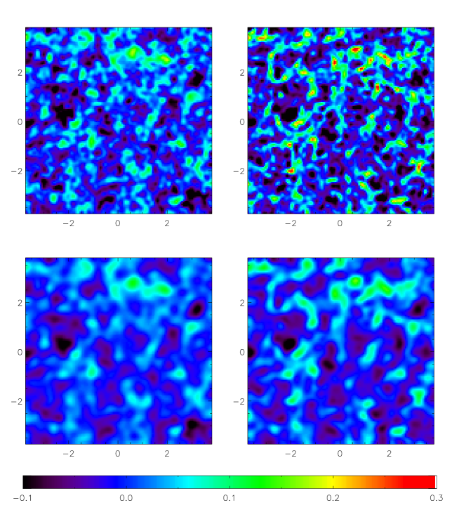
Figure 1: Maps of (left) input and (right) reconstructed projected mass, in units of dimensionless convergence $\kappa$, for two smoothing scales and $2\mu\rm K$-arcmin uncorrelated Gaussian instrument noise. While the (top) input and reconstructed $\kappa$ maps smoothed by a $10^{\prime}$ FWHM Gaussian beam do contain many of the same structures, the agreement between the two (bottom) visibly improves when they are smoothed on a $20^{\prime}$ scale. The input $\kappa$ maps shown here are Gaussian random fields, and all the maps are $7.5^{\circ}\times 7.5^{\circ}$.

An example of an input and reconstructed $\kappa$ map is given in Fig. 1. The raw maps are very noisy, so we have smoothed the convergence with a (upper panels) $10^{\prime}$ and (lower panels) $20^{\prime}$ FWHM Gaussian filter. Although $10^{\prime}$ is many times the nominal resolution used in the reconstruction, the estimated map made at this level of smoothing clearly leaves much to be desired. Increasing the smoothing to $20^{\prime}$ improves the reconstruction enough so that many of the features in the maps are reproduced, e.g. the overdensities at $(0^{\circ},3^{\circ})\rm{and}(-1^{\circ},-1^{\circ})$. The reconstruction is still noisy enough that some features, e.g. at $(3^{\circ},3^{\circ})$, are spurious.

It seems clear from Fig. 1 that if a reconstruction of the projected mass back to the surface of last scattering using only CMB temperature information is to be achieved, it can only be on large angular scales. This means averaging the density not only over the $10\,$Gpc along the line-of-sight but also over $100\,$Mpc transverse to it. Since we do not expect structures on these scales to be particularly informative, we shift our attention to the following statistical measures of the convergence field:

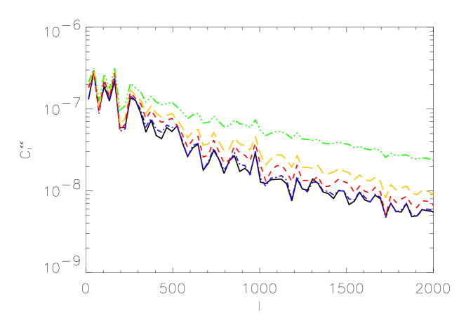
Figure 2: Reconstruction of the power spectrum for a Gaussian convergence map. The input $C_{\ell}^{\kappa\kappa}$ convergence spectrum (black) is poorly reconstructed, as is clear in the auto-spectrum (green) if noise terms are not subtracted. The situation improves markedly as the noise is subtracted to first order (orange), and still more when second order terms are subtracted (red), while the cross-spectrum (blue) fit is quite good.

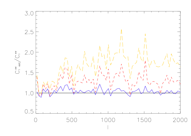
Figure 3: The ratio of the reconstructed power spectra to the input spectrum for a Gaussian $\kappa$ map (the spectra themselves are given in Fig. 2). The ratio for the cross-spectrum case (blue) is consistent with a no multiplicative bias; however, as is evident from the plot of $C_{\ell}^{\rm est}$ (red), there is still a substantial ($\sim 25\%$) additive bias even when second order noise terms are included. If only the first order correction is included in the noise estimate (Eq. 10), the bias is close to $\sim 70\%$.

$$\ \ \ \ \ \ \ \ \ \ \ \ \ \ \ \ \ \ \ \ \ \ \ \ \ \ \langle\kappa(\mbox{\boldmath$\ell$})\kappa^{*}(\mbox{\boldmath$\ell$}^{\prime})\rangle =2\pi\delta(\mbox{\boldmath$\ell$}-\mbox{\boldmath$\ell$}^{\prime})C_{\ell}^{\kappa\kappa}$$

$$\langle\kappa_{\rm est}(\mbox{\boldmath$\ell$})\kappa^{*}_{\rm est}(\mbox{\boldmath$\ell$}^{\prime})\rangle =2\pi\delta(\mbox{\boldmath$\ell$}-\mbox{\boldmath$\ell$}^{\prime})C_{\ell}^{\rm auto}$$

$$\langle\kappa_{\rm est}(\mbox{\boldmath$\ell$})\kappa^{*}(\mbox{\boldmath$\ell$}^{\prime})\rangle =2\pi\delta(\mbox{\boldmath$\ell$}-\mbox{\boldmath$\ell$}^{\prime})C_{\ell}^{\rm cross}$$ (7)

where $C_{\ell}^{\kappa\kappa}$ is the power spectrum of the input $\kappa$ map, $C_{\ell}^{\rm auto}$ is the auto-spectrum of the estimated map, and $C_{\ell}^{\rm cross}$ is the cross-correlation spectrum between the input and estimated convergence. Of these, only $C_{\ell}^{\rm auto}$ is in principal observable, but we will make use of all 3 to diagnose the quality of the reconstruction.

We generically expect that any estimator of $\kappa$ will have both an uncorrelated noise term $n_{\ell}$ and a multiplicative bias term $b_{\ell}$ associated with it, so that

$$\kappa_{\rm est}(\mbox{\boldmath$\ell$})=b_{\ell}\kappa(\mbox{\boldmath$\ell$})+n_{\ell}$$ (8)

If the estimator is properly normalized by $A_{\ell}$ as defined in Eq. 6, then the multiplicative term $b_{\ell}=1$, and the estimator is unbiased. On the other hand, $C_{\ell}^{\rm auto}$ is simply related to the input power spectrum $C_{\ell}^{\kappa\kappa}$ via the noise power $\mathcal{N}_{\ell}$ as $C_{\ell}^{\rm auto}=C_{\ell}^{\kappa\kappa}+\mathcal{N}_{\ell}$, so that our estimate $C_{\ell}^{\rm est}$ of $C_{\ell}^{\kappa\kappa}$ is

$$C_{\ell}^{\rm est}=C_{\ell}^{\rm auto}-\mathcal{N}_{\ell}^{\rm est}$$ (9)

where $\mathcal{N}_{\ell}^{\rm est}$ is the the estimated noise power. Thus, even if the normalization $A_{\ell}$ is correct, so that multiplicative bias is not an issue, an unbiased estimate of $C_{\ell}^{\kappa\kappa}$ requires that we know the noise power in the map so that we can account for the additive bias $\mathcal{N}_{\ell}$. Fortunately, Cooray & Kesden (2003) have shown that it is possible to estimate the noise as

$$\mathcal{N}_{\ell}^{\rm est}={\ell^{2}\over 4}\left(A_{\ell}+A_{\ell}^{NG}+\cdots\right)$$ (10)

where $A_{\ell}$ is the normalization of Hu (2001a), $A_{\ell}^{NG}$ is an additional signal dependent term (Eq. 12), and $\cdots$ represents higher order terms. We will define any failure to properly estimate the noise contribution $\mathcal{N}_{\ell}$ by $\mathcal{N}_{\ell}^{\rm est}$ as an additive bias.

Although $C_{\ell}^{\rm cross}$ is not measurable, we can still make use of it as a diagnostic of our estimate. Specifically, since

$$\langle C_{\ell}^{\rm cross}\rangle=b_{\ell}C_{\ell}^{\kappa\kappa}$$ (11)

we will be able to identify a multiplicative bias, caused by a failure of $A_{\ell}$ to properly normalize the estimator, and an additive bias, which exists when we are unable to determine the noise power in the reconstruction.

We display these power spectra in Fig. 2, and for clarity, we include the same information in the ratio plot shown in Fig. 3. It is clear from these plots that the (blue) cross spectrum $C_{\ell}^{\rm cross}$ traces the (black) convergence power spectrum $C_{\ell}^{\kappa\kappa}$, so the quadratic estimator is not multiplicatively biased if $A_{\ell}$ (as defined in Eq. 6) is used for the normalization and the assumptions of the estimator are met.

However, we see in the same figures that using $\mathcal{N}_{\ell}^{\rm est}\simeq A_{\ell}$ will lead to a substantial additive bias ($\sim 70\%$). Thus, quantitatively, an accurate measure of $C_{\ell}^{\kappa\kappa}$ requires us to use the higher order corrections, which unfortunately depend on $C_{\ell}^{\kappa\kappa}$ itself. We have two options here. The first is to develop an iterative scheme to solve for $C_{\ell}^{\kappa\kappa}$. This is non-trivial because the estimate of $C_{\ell}^{\kappa\kappa}$ is so intrinsically noisy. Some heavy smoothing is required to regularize the procedure. We have instead decided to assume that a parameterized functional form for $C_{\ell}^{\kappa\kappa}$ would be available, along with a good enough first guess at the parameters that the bias can be accurately estimated. Specifically we compute the bias assuming the “true” spectrum used in constructing the simulation, and use the residual as an estimate of how well we do.

The next term in $\mathcal{N}_{\ell}$ beyond $A_{\ell}$ is given in Eq. 12, and labeled schematically in Eq. 10 as $A_{\ell}^{NG}$. This term reduces the additive bias in the reconstruction to about $25\%$. As the series appears to be converging, it is not unreasonable to expect that including more higher order terms in the computation of $\mathcal{N}_{\ell}$ would reduce this discrepancy even further. We have not chosen to pursue this calculation here; other factors, such as the effect of non-Gaussianity in the $\kappa$ map and the contribution of the kSZ, are shown below to enter at a level equal or greater than these higher order “Gaussian approximation” terms (also, the computational resources required are non-trivial; see Section A.1). In the next section, we address these effects for our fiducial deep integration survey, and then in Section 5 we consider what we have learned in the context of ACT, APEX-SZ, Planck, and SPT.

4 Some Complicating Factors

So far, we have considered the reconstruction of the projected mass distribution under the simplifying assumption that the convergence and the noise are uncorrelated Gaussian fields. In this section, we explore some complicating factors, first by modifying the lensing field in Section 4.1, and then by including a pernicious foreground, the kSZ, in Section 4.2.

4.1 The Effect of a Non-Gaussian $\kappa$ Field

In this section we examine the impact of introducing non-Gaussianity into the mass distribution. We do this by creating a convergence map using an N-body simulation to model structures at $z<2$ (structures at higher redshift are modeled by a Gaussian random field as before.) We show the resulting $\kappa$ map and its reconstruction in the upper panels of Fig. 4. The maps have been smoothed by a $20^{\prime}$ window, and on this scale many of the prominent features in the recovered map look quite similar to the “real” ones. We can be more quantitative by considering the difference map of the the input and reconstructed fields, which we find is not well correlated with the input map. However, the distribution of this “noise” map is mildly non-Gaussian (slightly skew positive) and also not quite consistent with a “white noise” approximation.

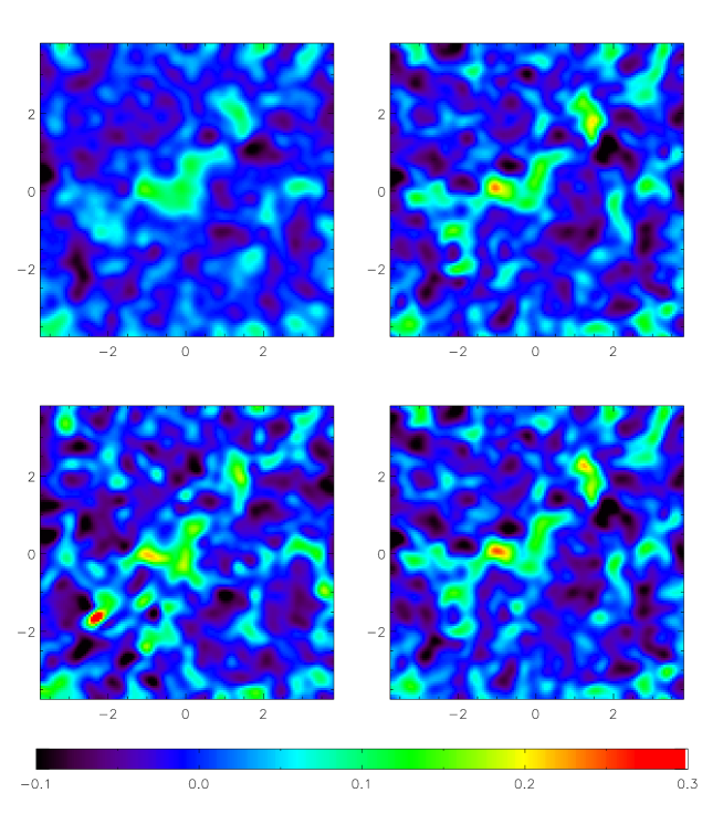
Figure 4: Reconstructions of a (top left) input non-Gaussian $\kappa$ map. The (top right) map has been reconstructed in the absence of foregrounds, and while it clearly contains much of the same structure as the input map, the correspondence is far from perfect, as we discuss in Section 4.1. When the kSZ is included, the (bottom left) reconstruction still retains some visual similarity to the original, although additional spurious features are added to the map, such as the hot spot near $(-2^{\circ},-2^{\circ})$. In the last panel we show the (bottom right) reconstruction when the kSZ is masked using the technique described in Section 4.2. The worst of the spurious structures caused by the kSZ have disappeared, and the map bears a strong resemblance to the reconstruction made in the absence of kSZ. The maps are $7.5^{\circ}\times 7.5^{\circ}$ fields sampled at $0.^{\prime}8$ resolution, include $2\mu$K-arcmin of instrument noise, and have been smoothed by a $20^{\prime}$ FWHM Gaussian window for presentation.

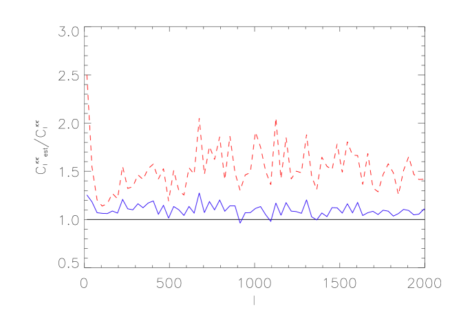
Figure 5: As Fig. 3, but now including the non-Gaussian contribution to the $\kappa$ map. The cross-spectrum (blue) is now biased high by roughly $10\%$, and the total bias in the estimated convergence spectrum (red) is about $50\%$.

To get a better idea of the properties of the estimated map, we once again turn to the convergence power spectrum $C_{\ell}^{\kappa\kappa}$. The ratio of the cross spectrum to the power spectrum $C_{\ell}^{\rm cross}/C_{\ell}^{\kappa\kappa}$ is shown as the blue (solid) line in Fig. 5, and indicates that the map is now multiplicatively biased high by $\sim 10\%$. This bias is not unexpected, because higher order moments of the field, which vanished in the Gaussian case, can now contribute (see Appendix). The red (dashed) line on the same plot, the ratio of the estimated power spectrum $C_{\ell}^{\rm est}/C_{\ell}^{\kappa\kappa}$ (including all the corrections considered in Section 3), shows a total bias of about $50\%$.

In addition to the excess power on the scales of interest (larger than 6 arcminutes), the reconstructed maps tend to have too little power on smaller scales (smaller than 2-3 arcminutes, not visible on the map). This decrement on very small scales is of similar size to the increment on larger scales ($\sim 10\,-\,20\%$). This is not surprising, given that the quadratic estimator has been optimized for a Gaussian field, and other reconstruction methods based on Gaussian assumptions (e.g. a Wiener filter) will typically mix power onto large scales from features that are too sharp to fit the Gaussian approximation.

4.2 Kinetic SZ Contamination

In this section, we will consider one more wrinkle in the reconstruction: foreground removal. While it may be that point sources or diffuse foregrounds will place real-world limits on how well we can reconstruct the lensing signal, in principle the only foregrounds we cannot distinguish from the CMB spectrally are the kinetic Sunyaev-Zel’dovich effect (kSZ), and its related cousin, the Ostriker-Vishniac (OV) effect (Ostriker & Vishniac, 1986). Of the two, the kSZ is likely to be more troublesome, since it is highly non-Gaussian and correlated to the lensing signal. Therefore, we will address only the kSZ here, although we note that this may be somewhat optimistic.

As we discuss in Section A.2, we create the kSZ signal using the same N-body simulation that we used to make the lensing maps. This is then added to the lensed CMB map, which is used to reconstruct the convergence $\kappa$. The resulting map, shown in the (bottom left) panel of Fig. 4, is clearly substantially degraded, as the strongest kSZ sources (Fig. 7), e.g. the “hot spot” at $(-2^{\circ},-2^{\circ})$, now appear in the reconstructed map. The contamination is even more prominent in the estimated convergence power spectrum $C_{\ell}^{\rm est}$, which is now biased high by well over a factor of 2!

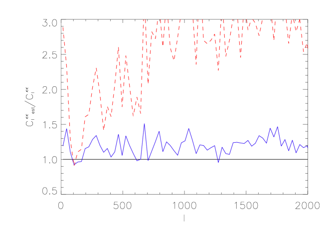
Figure 6: As Fig. 3, but now including effects from both the kSZ and the non-Gaussian $\kappa$ field. The cross spectrum (blue) is now biased by 20%, while for the estimated convergence spectrum (red), the bias from the kSZ signal completely overwhelms the signal.

Since the kSZ is concentrated around large clusters, one obvious idea to correct for the effect is to “mask” the major clusters using a measurement of the thermal SZ. As a simple check of this technique, we used a 50$\mu$K (at 150 GHz) thermal SZ temperature threshold to cut pixels from the “observed” CMB temperature map. This resulted in our excising roughly $1.4\%$ of the pixels from the map, as shown in Fig. 7. We then replace the “holes” by interpolating the surrounding area using the two variable method of Renka & Cline (1984). The interpolated map does not contain obvious numerical artifacts associated with the masking process.

Before we proceed with reconstructions using these masked maps, we need to check whether the procedure has significantly reduced the lensing signal by limiting the contribution from clusters. We do this by masking and interpolating the lensed temperature map, but without adding the kSZ, and then computing the power spectrum. We find that the 1.4% cut we have used results in only a modest (slightly less than 5%) reduction of the lensing signal. Two issues are likely to be responsible for mitigating the masking effect on the lensing power. First, the lensing signal extends to larger angular scales than the kSZ, and second, much of the lensing power comes from lower mass halos which we don’t mask.

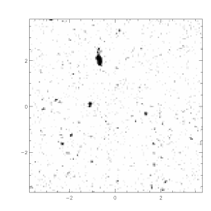
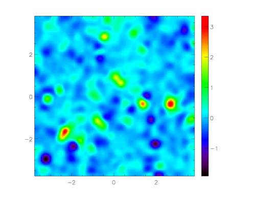
Figure 7: An illustration of the masking and interpolation techniques we use to control the kSZ. Regions with a thermal SZ temperature magnitude in excess of $50\mu K$ (left) are masked, resulting in a loss of only 1.4% of the pixels in the map. This can be compared to the (smoothed) kSZ map (right).

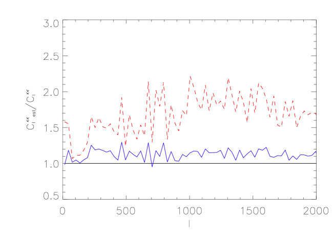
Figure 8: As in Fig. 6, but the kSZ has been masked, as described in the text. The cross-spectrum (blue) is down to a bias of $\sim 15\%$, which is only slightly higher than when no kSZ is included. The bias in $C_{\ell}^{\kappa\kappa}$ (red) is reduced but still significant.

In any case, a small reduction in signal is an acceptable price to pay if we can control the large error introduced by the kSZ. Indeed, the map made using this correction is greatly improved; as we show in Fig. 4, the spurious features have largely disappeared in the reconstruction, and the map made using masking is visually very similar to the reconstructed map made without including any kSZ at all.

The estimate of the power spectrum $C_{\ell}^{\rm est}$ also shows substantial improvement, and is now biased by only roughly $70\%$. Although this is considerably better than the unmasked case, there is obviously still a residual kSZ contribution of about $20\%$, which may arise from the kSZ which is uncorrelated to the lensing signal. There may also be a similar effect due to Ostriker-Vishniac fluctuations from $z>2$, but we have not studied this issue here.

It is clear that the kSZ is an important foreground which cannot safely be ignored when considering CMB lensing effects, and that the masking technique we have used here is a step forward. We have not attempted to optimize the process, so it is not clear to what extent the masking procedure can be tuned to further reduce the contamination of the lensing signal.

5 Noise and Bias for Upcoming Surveys

In this section we shall model the reconstruction that may be possible from a number of upcoming experiments. Our conclusions will be overly optimistic in that they ignore systematic effects and incomplete foreground removal, but they serve to illustrate the role of noise levels and resolution which can be achieved in the next 5 years.

5.1 The Impact of Improving Angular Resolution

Until now, we have considered a high-sensitivity, high angular resolution fiducial experiment, which has led us to find substantial biasing effects related to the ability of the experiment to resolve small structures. In this section, we show the effect that improving the angular resolution has on the biases and on the signal-to-noise. We compute the estimated convergence power-spectrum for different levels of angular resolution, keeping the noise level at a constant $2\mu$K-arcmin, and find that both the map bias (multiplicative bias $C_{\ell}^{\rm cross}/C_{\ell}^{\kappa\kappa}$) and the noise estimate bias (additive bias $C_{\ell}^{\rm est}/C_{\ell}^{\kappa\kappa}$) decrease as the beam size increases (Fig. 9).

Figure 9: Additive (dotted line) and multiplicative (dashed line) average bias produced by the non-Gaussianity in the convergence field versus the resolution of the experiment, the solid line represents the average signal-to-noise ratio (square root of the signal variance over the noise variance). The averages are computed between $\ell=0$ and $\ell=2000$. The bias decrease with the resolution, but reducing the bias lowers the sensitivity.

The price of decreasing the bias is a much lower signal-to-noise ratio (Fig. 9), which is reduced on average by a factor 3 when the resolution is degraded by a factor 5. Furthermore, this lower angular resolution leads to a cutoff in $\ell$ space (Fig. 10; 4 arcminute resolution cuts the S/N at $\ell\sim 1000$) as the S/N is not constant in $\ell$. We got similar results by low-pass filtering the data of 0.8 arcminute beam (this corresponds to change artificially the “optimal” filter), this easy solution to reduce the bias degrades also the signal-to-noise ratio. Adding the noise level as an another free parameter, one may find an optimal (or several) values of the noise level and angular resolution which minimize bias from non-Gaussianity in the convergence field and maximize the average S/N. This preliminary study suggests that a middle range angular resolution experiment (around 4 to 5 arcminutes), with a big sky coverage and a great sensitivity will be best suited to accomplish this.

Figure 10: Signal-to-noise ratio versus angular scale for several angular resolutions (respectively 0.8, 1.6, 2.4, 3.6, 4 arcminutes for the solid, dotted, dashed, dot-dashed, triple dot-dashed lines). The signal-to-noise ratio decreases with the angular resolution especially at small angular scales.

5.2 Estimated Reconstructions for Upcoming Surveys

In this section, we consider four upcoming surveys which possess enough sensitivity to supply a first detection of the CMB lensing effect : APEX/SZ, ACT, SPT and Planck. We reconstruct the convergence from a CMB temperature map, which is made using a non-Gaussian lensing field, and includes contamination from the kSZ. We include instrument effects appropriate to each experiment, and treat the kSZ in the maps using our “masking” correction technique. Small regions ($7.5^{\circ}\times 7.5^{\circ}$) of reconstructed $\kappa$ are displayed in Fig. 11, and the estimated power spectra are given in Fig. 12.

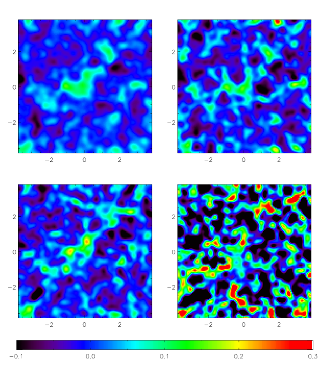
Figure 11: Reconstructed maps of the convergence $\kappa$, from top to bottom and left to right : input convergence map, APEX/SZ, SPT, Planck reconstructed convergence map smoothed by a 20’ FWHM Gaussian. The maps represent a $7.5\times 7.5$ degree chunk of each simulations. As the noise level worsen the structures became less and less recognizable. In Planck case, the map is completely dominated by noise on these scales.

For APEX/SZ, we use a sensitivity of 8 $\mu$K-arcmin on a $15^{\circ}\times 15^{\circ}$ field with a $0.^{\prime}8$ angular resolution. Note that these characteristics are sufficiently similar to those of ACT (5.7 $\mu$K/arc² sensitivity on a $15^{\circ}\times 15^{\circ}$ field with a $1.^{\prime}1$ angular resolution) that we refer the reader to the same plots for ACT as for APEX/SZ. The estimated convergence map is noisy, but the main features are recognizable. Therefore APEX/SZ may well be the first experiment to detect the CMB lensing effect. The surveys should also be sensitive enough to place some limits on the power spectrum, although the estimates will suffer from a non-negligible bias.

For the Planck satellite, we assume a 65 $\mu$K-arcmin sensitivity, a $5^{\prime}$ resolution, and analyse only a $60^{\circ}\times 60^{\circ}$ field (about 1/10^th of Planck coverage) to remain in the flat sky approximation. The reconstructed small scale convergence map is completely dominated by noise, as expected and would also be true for a full sky map. Using our masking technique the bias in Planck reconstruction seems to be quite negligible, though our contrains on the bias residual is limited by our small sky coverage. The full sky coverage will reduce the error bars presented on Fig. 12, but the convergence power spectrum estimate will be cut off at small scales ($\simeq$ 1000) due to the large size of the beam.

For SPT, we assume a 10 $\mu$K-arcmin sensitivity on a $60^{\circ}\times 60^{\circ}$ field with a $1^{\prime}$ angular resolution. The higher noise level makes the structures harder to recognize, although it is still possible to identify many of them. The result for the power spectrum is markedly better than the other surveys we are considering; the combination of low noise, small beam, and large survey area combine to perform relatively well at this task.

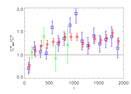
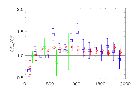
Figure 12: Ratio of the estimated convergence power spectrum with the input one for APEX/SZ (blue squares), SPT (red diamonds), 1/10^th of Planck (green crosses). The values are binned in $\Delta\ell=120$, except for Planck ones which are binned in twice bigger $\Delta\ell$ (the Planck points stop at $\ell=1000$ as we get a poor reconstruction on smaller scales). The unmasked power spectrum estimation (left) is biased on average by 30%, whereas the masked power spectrum estimation (right) is biased by only 10%. Note that we have simulated only about one tenth of the sky, so that the error bars on the Planck estimate appear larger than they should.

For the conditions we have assumed, all of these experiments will detect the lensing effect and measure the convergence power spectrum on scales ranging from a few degrees to a few arcminutes. However, although the masking technique shows promise for reducing this contamination, even if the procedure was not optimized, the kSZ bias remains significant for APEX/SZ, ACT and SPT. Our investigations suggest that very low noise and large sky coverage are the two main drivers for lensing reconstruction.

6 Discussion

Lensing of CMB photons may provide a window into the matter distribution projected from primordial times to the present. A great deal of work has been put into developing the statistical methods needed to fulfill this promise, and our goal here has been to further these efforts. To this end, we have extensively checked the power and assumptions of one of the two principal estimators that have emerged, the “optimal” quadratic estimator of Hu (2001a), both for reconstructing projected mass maps and for measuring the matter power spectrum. Although our results apply specifically to the quadratic estimator, we note that the other principal candidate (the maximum likelihood estimator of Hirata & Seljak, 2003a) makes the same assumptions about the underlying fields as the quadratic estimator, so it is likely to face the same challenges.

We began our efforts in Section 3, where we tested the quadratic estimator method under the artificial conditions of a Gaussian gravitational potential, and uncorrelated Gaussian noise, for which the estimator is most likely to succeed. The noise in the reconstructed maps has $\kappa$ dependent extra terms which constitute an additive bias in power spectrum measurements. The second order terms were discussed in (Cooray & Kesden, 2003), and we confirm their prediction that these are numerically significant. In addition, we find for the first time that higher order terms are also likely to be significant, since these second order terms do not fully correct bias for interesting observational parameters. Although the bias is signal dependent, it may be possible to correct for this fact by using iterative methods or model fits, as suggested by Kesden, Cooray, & Kamionkowski (2003); however, high order terms would need to be included to obtain good accuracy.

It is clear that a reconstruction method based on the assumption of a Gaussian lensing field will not optimally treat non-Gaussian features, such as clusters, which contain more information than just the 2-point function. We investigated this issue in Section 4.1 by using a lensing field generated from an N-body simulation. This imposed both a multiplicative bias on the cross spectrum estimate, and an additional additive bias on the auto spectrum. The bias increased as the signal-to-noise ratio increased.

We investigated the impact of a second non-Gaussian complication, the kinetic Sunyaev-Zel’dovich effect (kSZ), in Section 4.2. This “noise” is highly correlated with the lensing signal and, unlike the larger thermal SZ, is impossible to distinguish from the CMB using spectroscopic methods. We began by showing that, if left untreated, this effect will completely dominate the reconstruction. One obvious method to correct for this is to use a measurement of the thermal SZ (which is correlated with the kSZ) to mask pixels which are likely to have a large contamination, and we were able to substantially reduce the bias caused by the kSZ while excising only a relatively small number of pixels. Although this was encouraging, not all of the kSZ signal is correlated with the thermal SZ and the contamination level remained significant. Further reduction of kSZ noise by simply masking more pixels suffers from steadily decreasing returns in signal-to-noise improvement. We suspect, although we have not checked it explicitly, that contamination from the Ostriker-Vishniac effect would behave in a similar manner.

Given the difficulty that one encounters using Gaussian reconstruction methods, it is natural to ask if the non-Gaussian nature of the lensing signal might itself provide the best probe of the lensing field. This topic has recently been the subject of great interest in the context of galaxy lensing (e.g. Takada & Jain, 2003; Zaldarriaga & Scoccimarro, 2003; Ho & White, 2003), but to this point a similar effort is lacking for lensing of the CMB. There is clearly promise in this idea; however, any measurement of the non-Gaussian signal is likely to be particularly sensitive to the masking technique needed to control the kSZ, which will be highly correlated with this signal. For example, clusters will produce both a large non-Gaussian lensing signal and a large kSZ in the same location, at the cluster. Thus, it may be necessary to mask precisely those pixels which would otherwise have provided the best window into the non-Gaussian signal.

In this paper, we have been primarily interested in the reconstructions that can be accomplished using the unprecedented power and resolution that will be available in the next generation of surveys, and it is in this context that biasing effects emerge as important obstacles. In the regime of large smoothing and low signal-to-noise, the bias due to non-Gaussian effects is small, and the quadratic estimator performs well in this regime. It is only when the observational parameters are improved that the biasing effects we have been discussing emerge. We show in Fig. 9 the unfortunate increase in bias that occurs as signal-to-noise is improved, so that a recovery of the power spectrum can have either small error bars or negligible bias, but not both. Thus, while a detection of the lensing effect is likely to be achieved by APEX/SZ, more ambitious goals that rely on extremely high fidelity reconstructions of the matter power spectrum require significantly more modeling.

We have presented a number of reconstructed maps in this paper, and it is clear that features in these maps do coincide with the those of the original fields at some level. However, we note that the maps have been smoothed by a $20^{\prime}$ FWHM Gaussian window, and even so the reconstructed maps are far from perfect. We have also performed extensive numerical integrations to compute the corrections to the noise term $\mathcal{N}_{\ell}$ outlined in Section 3. Although these corrections proved useful for for removing some of the bias effects, the computational power needed for this calculation is non-trivial, a point which we discuss in more detail in the Appendix.

Although we have not treated the issue here, we would like to make some comments about the role of polarization in CMB lensing. It has been emphasized (Guzik, Seljak, & Zaldarriaga, 2000; Hu & Okamoto, 2002; Cooray & Kesden, 2003; Hirata & Seljak, 2003b; Kesden, Cooray, & Kamionkowski, 2003; Okamoto & Hu, 2003) that the inclusion of polarization information might dramatically enhance the prospects for large-scale structure reconstruction from lensing of the CMB. This is because lensing induces a $B$-mode polarization signal which is otherwise absent for purely scalar, primary fluctuations. The large intrinsic primary CMB anisotropies, which are a source of “noise” for lensing reconstruction, are thus absent. However, the spatial structure is complicated for polarization, as it is for temperature, and the signal levels are much smaller. The kSZ effect, which is one of our major contaminants, is also polarized (Sunyaev & Zel’dovich, 1980b). Thus, although it is certainly reasonable that the addition of polarization information would enhance the prospects for $C_{\ell}^{\kappa\kappa}$ reconstruction, a detailed calculation is required to determine how much better one can actually do.

Weak lensing is one of the principal tools for cosmologists, and promises to be increasingly significant for many years to come. Lensing of the CMB is a new addition to the arsenal, which will be facilitated by powerful upcoming surveys such as ACT, APEX-SZ, Planck, and SPT. Even as observers gear up to probe the millimeter and sub-millimeter wavebands with unprecedented power and resolution over large fractions of the sky, theorists continue to improve the methods necessary to extract relevant information from the resulting measurements. If the pace of development on both fronts continues at its current rate, the future looks bright indeed.

Acknowledgments:
A.A. would like to thank the organizers of the workshop “Cosmology with Sunyaev-Zel’dovich cluster surveys” held in Chicago in September 2003 for allowing him the chance to present some of this work. Additionally we would like to thank T. Chang, J. Cohn, M. Zaldarriaga for helpful discussions about these results. The simulations used here were performed on the IBM-SP2 at the National Energy Research Scientific Computing Center. This research was supported by the NSF and NASA.

Appendix A Appendix: Numerical Issues

A.1 Computing the Quadratic Estimator

In this section, we discuss some of the issues associated with computing the quadratic estimator of Hu (2001a) and the higher order corrections we have considered in this paper. One of the advantages of the estimator is that it is inexpensive to compute, but higher order terms add to the difficulty, as we discuss below.

The lensing effect can be expressed as a Taylor expansion (Eq. 3) of the unlensed temperature. If the deflection angle $\delta\mbox{\boldmath$\theta$}$ is small enough, then the linear approximation is valid, and the normalization $A_{\ell}$ (Eq. 6) of the optimal quadratic estimator (Eq. 4) is a good approximation to the estimated convergence power spectrum noise term. In this case, the estimator requires as inputs the measured CMB temperature map and the power spectrum of the unlensed CMB. It is likely that a good estimation of the latter can be achieved by measuring cosmological parameters at large angular scales.

Cooray & Kesden (2003) explored terms to second order in the deflection angle. Although this resulted in the same estimator of $\kappa$, they found another significant term in the estimator $C_{\ell}^{\rm est}$ of the convergence power spectrum, in addition to the first order noise correction $A_{\ell}$. This term, $A_{\ell}^{NG}$, is defined as

$$\small{A_{\ell}^{NG}={A_{\ell}^{2}\over\ell^{2}}\int{d^{2}\ell_{1}\over(2\pi)^{2}}\int{d^{2}\ell_{2}\over(2\pi)^{2}}F(\mbox{\boldmath$\ell$}_{1},\mbox{\boldmath$\ell$}-\mbox{\boldmath$\ell$}_{1})F(\mbox{\boldmath$\ell$}_{2},\mbox{\boldmath$\ell$}-\mbox{\boldmath$\ell$}_{2})}$$ (12)

$$\footnotesize{\left\{C^{\phi\phi}_{|\mbox{\boldmath$\ell$}_{1}-\mbox{\boldmath$\ell$}_{2}|}f(-\mbox{\boldmath$\ell$}_{1},\mbox{\boldmath$\ell$}_{2})f(\mbox{\boldmath$\ell$}_{1}-\mbox{\boldmath$\ell$},\mbox{\boldmath$\ell$}-\mbox{\boldmath$\ell$}_{2})+C^{\phi\phi}_{|\mbox{\boldmath$\ell$}_{1}-\mbox{\boldmath$\ell$}+\mbox{\boldmath$\ell$}_{2}|}f(-\mbox{\boldmath$\ell$}_{1},\mbox{\boldmath$\ell$}-\mbox{\boldmath$\ell$}_{2})f(\mbox{\boldmath$\ell$}_{1}-\mbox{\boldmath$\ell$},\mbox{\boldmath$\ell$}_{2})\right\}}$$

where $F(\mbox{\boldmath$\ell$}_{1},\mbox{\boldmath$\ell$}_{2})$ is as in Eq. 5 and $f(\mbox{\boldmath$\ell$}_{1},\mbox{\boldmath$\ell$}_{2})={(\mbox{\boldmath$\ell$}_{1}+\mbox{\boldmath$\ell$}_{2})\cdot(\mbox{\boldmath$\ell$}_{1}\tilde{C_{\ell_{1}}}+\mbox{\boldmath$\ell$}_{2}\tilde{C_{\ell_{2}}})}$. This term is smaller than the $0^{\rm th}$ order term $A_{\ell}$, but it is not negligible; for example, it represented $\sim 35\%$ of the power for our fiducial low noise, high resolution survey used in Sections 3 and 4. The convergence of this integral and the one of equation 6 is provided by the noise level, so that the computation time increases as lower noise surveys are considered. However, the second order terms are not a problem for a modern workstation, and takes about 30 minutes of CPU time for a typical calculation.

The computation of Eq. 12 introduces a new challenge, in that this requires the potential power spectrum $C_{\ell}^{\phi\phi}$ as an input, which is of course the quantity we are trying to measure. Either an iterative procedure or a model fit might resolve this issue, and we have assumed (but not demonstrated) that this is possible, so that we use the actual input $C_{\ell}^{\phi\phi}$ for our computation of $A_{\ell}^{NG}$.

When we do this, the inclusion of $A_{\ell}^{NG}$ into the estimate of the power spectrum improves the bias issue substantially, but does not solve the problem. Additional terms may be required, so that the auto-spectrum of the map may include other terms, written schematically below as

$$C_{\ell}^{\rm auto}\simeq\left<T^{4}\left(a+b\kappa+c\kappa^{2}+d\kappa^{3}+e\kappa^{4}+\cdots+i\kappa^{8}\right)\right>$$ (13)

So far, by including $A_{\ell}$ and $A_{\ell}^{NG}$, we have considered the 0^th, 2^nd, and a part 4^th order terms in $\kappa$. Some of the terms we have ignored may be small enough to be irrelevant, and in the case of a Gaussian $\kappa$, the odd order terms should be null. However, our results in section 3 exhibit evidence for a non-negligible contribution from additional higher order terms. If $\kappa$ is a Gaussian field, $C_{\ell}^{\rm auto}$ can be written analytically, and in principle its noise contribution computed. However, the numerical challenge would be non-trivial. Since the $\kappa^{2}$ correction took $\sim 30$ minutes, we estimate that for the same resolution, the $\kappa^{4}$ would take 5,000 hours, and so on for higher orders. Furthermore, if $\kappa$ is a non-Gaussian field, then the odd order moments are not expected to be identically zero, and the higher order even moments can not be expressed as a function of the two point correlation function. In this case, numerical simulations will be needed to recover the convergence power spectrum.

A.2 The Simulations

In this paper, we have made extensive use of maps of the primary CMB temperature anisotropies, the convergence $\kappa$, and the thermal and kinetic SZ effects. Our technique for simulating these maps has been described in detail elsewhere (Vale, Amblard, & White, 2004), so we confine ourselves here to a brief discussion of some points directly relevant to this work.

We chose a fiducial flat, $\Lambda$CDM cosmology generally consistent with currently popular models, with $\Omega_{m}=0.3,\Omega_{\Lambda}=0.7,h=0.7,\Omega_{b}h^{2}=0.02,n=1,\sigma_{8}=1$. Maps of primary CMB temperature anisotropies were made as random realizations of a Gaussian field with a power spectrum computed using CMBfast (Seljak & Zaldarriaga, 1996). The CMB maps are $30^{\circ}\times 30^{\circ}$ square patches of sky containing $2048\times 2048$ pixels.

We made use of Gaussian convergence maps to account for the lensing effect of matter located at high redshift $z>2$, and for certain tests as outlined in the text. These were created from a random realization of a Gaussian field in much the same manner as the maps of the CMB, but using a power spectrum computed using the the non-linear growth factor described by Peacock & Dodds (1996) and the Limber approximation.

The other maps require some knowledge of the spatial distribution and time evolution of the mass in the model, which we obtain from an N-body simulation using the TreePM code described in White (2002). This simulation modeled a large volume of the universe, a cube $300\ h^{-1}\rm Mpc$ on a side, and used only dark matter, which was modeled using $512^{3}$ particles. This was then used to make maps of the convergence, the thermal SZ, and the kinetic SZ, for a distribution of matter out to a redshift $z=2$ and a field of view of $7.5^{\circ}\times 7.5^{\circ}$. The convergence map was made by a simple weighted sum of the line of sight density contrast and thus implicitly assumed the validity of the Born and Limber approximations (which was investigated in some detail in Vale & White, 2003). In order to compute the thermal and kinetic SZ effects, we assumed that the baryonic matter traces the dark matter, which is likely to be a good approximation on scales which can be resolved by our fiducial surveys. We refer the reader to (Schulz & White, 2003; Vale, Amblard, & White, 2004) for a complete description of this process.

The reader may have noticed that the CMB temperature maps are $30^{\circ}$ on a side, while maps made using the N-body simulation are only $7.5^{\circ}$ on a side. The reason for this discrepancy is that simulations that have the dynamic range to cover so large a field of view while maintaining sufficient small scale resolution require more computing power than we can muster. We could cover the field with patches made from different simulations, but this would create highly artificial boundaries. Our solution to this issue, as illustrated in Fig. 13, is to cover the $30^{\circ}\times 30^{\circ}$ patch of sky with sixteen $7.5^{\circ}\times 7.5^{\circ}$ tiles of a given field. These smaller patches are duplicates of the same field, but are oriented so that the resulting map avoids the structural discontinuities mentioned above. In this way we are able to create the large continuous periodic fields necessary to test reconstruction techniques.

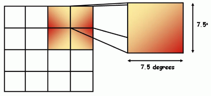
Figure 13: An illustration of the tiling technique we use to create a large ($30^{\circ}\times 30^{\circ}$) map from a smaller one. Maps of the convergence $\kappa$ and of the SZ effects are derived using the matter distribution from an N-body simulation with a $7.5^{\circ}\times 7.5^{\circ}$ field of view. To avoid artificial boundaries in the larger field, we cover it with sixteen tiles. The tiles are identical to one another and are oriented in a manner that assures a continuous field with periodic boundary conditions.

References

- (1)
- Bartelmann & Schneider (2001) Bartelmann, M., & Schneider, P., 2001, Phys. Rep., 340, 291-472
- Birkinshaw (1999) Birkinshaw M., 1999, Phys. Rep., 310, 98
- Carlstrom, Holder, & Reese (2002) Carlstrom J., Holder G., Reese E., 2002, ARAA, 40, 643
- Cooray (2002) Cooray A., Phys. Rev. D, 2002, 66,103509
- Cooray & Kesden (2003) Cooray A., Kesden, M., 2003, NewA, 8,231
- Guzik, Seljak, & Zaldarriaga (2000) Guzik J., Seljak, U., Zaldarriaga M., Phys. Rev. D, 2000, 62,043517
- Hirata & Seljak (2003a) Hirata, C.M., Seljak, U., 2003a, Phys. Rev. D, 67,043001
- Hirata & Seljak (2003b) Hirata, C.M., Seljak, U., 2003b, Phys. Rev. D, 68,083002
- Ho & White (2003) Ho S., White M., 2003, to be published in ApJ, preprint [astro-ph/0312253]
- Hu (2001a) Hu, W., 2001a, ApJ, 557, L79
- Hu (2001b) Hu, W., 2001b, Phys. Rev. D, 64, 083005
- Hu & Okamoto (2002) Hu, W., Okamoto, T., 2002, ApJ, 574, 566
- Kaplinghat, Knox, & Song (2003) Kaplinghat, M., Knox, L., Song, Y.-S., 2003, to be published in Phys. Rev. Lett., preprint [astro-ph/0303344]
- Kesden, Cooray, & Kamionkowski (2002) Kesden, M., Cooray A., Kamionkowski, M., 2002, Phys. Rev. D, 66,083007
- Kesden, Cooray, & Kamionkowski (2003) Kesden, M., Cooray A., Kamionkowski, M., 2003, Phys. Rev. D, 67,123507
- Okamoto & Hu (2002) Okamoto, T., Hu, W., 2002, Phys. Rev. D, 66,063008
- Okamoto & Hu (2003) Okamoto, T., Hu, W., 2003, Phys. Rev. D, 67, 083002
- Ostriker & Vishniac (1986) Ostriker J., Vishniac E., 1986, ApJ, 306, L51
- Peacock & Dodds (1996) Peacock, J.A., Dodds, S.J., 1996, MNRAS, 280, 19
- Renka & Cline (1984) Renka, R.L., Cline, A.R., 1984, Rocky Mountain J. Math., 14, 223
- Rephaeli (1995) Rephaeli, Y., 1995, ARA&A, 33, 541
- Seljak (1996) Seljak, U., 1996, ApJ, 463, 1
- Seljak & Zaldarriaga (1996) Seljak U., Zaldarriaga M., 1996, ApJ, 469, 437
- Seljak & Zaldarriaga (2000) Seljak U., Zaldarriaga M., 2000, ApJ, 538, 57
- Schulz & White (2003) Shulz A., White M., 2003, ApJ, 586, 723
- Sunyaev & Zel’dovich (1972) Sunyaev R.A., Zel’dovich Ya. B., 1972, Comm. Astrophys. Space Phys., 4, 173
- Sunyaev & Zel’dovich (1980a) Sunyaev R.A., Zel’dovich Ya. B., 1980a, ARA&A, 18, 537
- Sunyaev & Zel’dovich (1980b) Sunyaev R.A., Zel’dovich Ya. B., 1980b, MNRAS, 190, 413
- Takada & Jain (2003) Takada M., Jain B., 2003, MNRAS, 344, 857
- Tegmark (1997) Tegmark M., 1997, Phys. Rev. D, 55, 5895
- Vale & White (2003) Vale C., White M., 2003, ApJ, 592, 699
- Vale, Amblard, & White (2004) Vale C., Amblard A., White M., 2004, preprint [astro-ph/0402004]
- van Waerbeke & Mellier (2003) van Waerbeke L., Mellier Y., 2003, preprint [astro-ph/0305089]
- White (2002) White M., 2002, ApJS, 143, 241
- Zaldarriaga & Scoccimarro (2003) Zaldarriaga, M., Scoccimarro, R., 2003, ApJ, 584, 559
- Zaldarriaga & Seljak (1999) Zaldarriaga, M., Seljak, U., 1999, Phys. Rev. D, 59,123507
- Zaldarriaga (2000) Zaldarriaga, M., Phys. Rev. D, 62, 063510