200 Mpc Sized Structure in the 2dF QSO Redshift Survey

Abstract

The completed 2dF QSO Redshift (2QZ) Survey has been used to search for extreme large-scale cosmological structure ($\sim$200 h^-1 Mpc) over the redshift range $0<z<2.5$. We demonstrate that statistically significant overdensities and underdensities do exist and hence represent the detection of cosmological fluctuations on comoving scales that correspond to those presently detected in the cosmic microwave background. However, the fractional overdensities on scales $>100$ h^-1 Mpc are in the linear or only weakly non-linear regime and do not represent collapsed non-linear structures. We compare the measurements with the expectation of the $\Lambda$CDM model by measuring the variance of counts in cells and find that, provided the distribution of QSOs on large scales exhibits a mild bias with respect to the distribution of dark matter, the observed fluctuations are found to be in good agreement with the model. There is no evidence on such scales for any extreme structures that might require, for example, departures from the assumption of Gaussian initial perturbations. Thus the power-spectrum derived from the 2QZ Survey appears to provide a complete description of the distribution of QSOs. The amount of bias and its redshift dependence that is required is consistent with that found from studying the clustering of 2QZ QSOs on $\sim$10 h^-1 Mpc scales, and may be adequately described by an approximately redshift-invariant power spectrum with normalisation $\sigma_{8}\simeq 1.0$ corresponding to a bias at $z=0$ of $b\simeq 1.1$ rising to $b\simeq 2$ at the survey’s mean redshift $z\simeq 1.5$.

1 Introduction

It has long been recognised that active galaxies and QSOs may used to probe structure in the universe on the largest observable scales, and statistical analysis of the clustering of samples of such cosmological objects was first developed thirty years ago (e.g. Webster 1976; Seldner & Peebles 1978). Even in those early studies it became apparent that, although the universe appeared generally homogeneous on the largest scales, individual clusters of active galaxies could be identified (Webster, 1982). In modern ideas of active galaxies and of their link to the process of galaxy formation, it is now thought that luminous QSOs lie at the heart of the most massive elliptical galaxies (Kukula et al. 2001; Dunlop et al. 2003; Floyd et al. 2003) and that, provided the clustering bias expected for such a population is accounted for (Sheth & Tormen, 1999), studying the clustering of active galaxies is a means of testing the predictions of hierarchical galaxy formation theory both on the largest cosmological scales and as a function of cosmic epoch.

Whether non-uniform distributions of QSOs on large scales could in fact be detected with a high degree of statistical confidence was an open question for many years, however, largely because of the limited sample sizes and systematic uncertainties and varying selection biases present in samples of QSOs. A statistically significant detection of QSO clustering on $\sim$10 Mpc scales was achieved primarily from the AAT QSO redshift survey (Shanks & Boyle, 1994). With the advent of the much larger 2dF QSO Redshift Survey (2QZ: Croom et al. 2001a; Smith et al. 2004; Croom et al. 2004b) not only has an extremely secure detection of QSO clustering been achieved, but also the shape of the correlation function, its bias with respect to the underlying dark matter distribution, the cosmic evolution in that bias, and the luminosity dependence of QSO clustering have now all been measured on scales out to about 80 Mpc (Croom et al. 2001b, 2002, 2004a, 2005).

On larger scales, the shape of the power spectrum of QSO clustering has been measured and shown to be consistent with the expectations for a low density CDM universe (Outram et al., 2003). The aim of this paper is to look at the distribution of QSOs in redshift space, rather than Fourier; to investigate on what scales departures from randomness may be detected; and to test whether those departures are consistent with the expectation of the widely-assumed cosmological model in which structures have grown by gravitational collapse of initially Gaussian fluctuations in a universe dominated by a combination of cold dark matter and dark energy. Over the years there have been a number of claims of the detection of extremely large (50–200 Mpc) groupings of AGN and QSOs (Crampton et al., 1987; Clowes & Campusano, 1991; Williger et al., 2002; Brand et al., 2003): at the time of these claims there was no consensus on the cosmological model or on the relationship of the distribution of QSOs to the distribution of matter, and it was hoped that the measurement of such large groupings might constrain models of one or both of these. Now, however, there have emerged in the literature preferences for one particular cosmological model (Spergel et al., 2003) and for the bias of QSOs measured by the 2dF QSO Redshift Survey (Croom et al., 2001b, 2002, 2004a, 2005), so it is timely to ask whether the very large scale distribution of QSOs is consistent with these recent developments. If such large-scale clusters were shown to be collapsed structures with high values of overdensity this would be likely to be in significant disagreement with the cosmological model and measurements of QSO bias. In fact, we shall see in this paper that indeed very large groupings of QSOs may be identified, possibly on scales as large as 300 Mpc, but that the groupings are still in the linear regime of gravitational collapse and are in fact entirely in accord with current expectations.

2 Analysis of the 2QZ survey

2.1 The 2QZ survey

The 2QZ survey is described by Croom et al. (2001a); Smith et al. (2004); Croom et al. (2004b). It comprises spectroscopic observations of blue colour-selected QSOs in two sky areas totalling 740 deg²: one a strip 5 degrees in declination by 75 degrees in right ascension passing through the south Galactic pole (the “SGP” region) and the other a similar-sized strip on the celestial equator in the region of the north Galactic cap (the “NGP” region). In this paper we analyse each region separately in order to test for systematic errors or differences between the two halves. Spectroscopic observations at $b_{J}>18.25$ were carried out with the 2dF facility at the Anglo-Australian telescope, brighter candidates were observed with the 6dF facility at the U.K. Schmidt Telescope operated by the Anglo-Australian Observatory but are not included in this analysis. The survey contains 21,181 “Quality 1” QSOs with $0<z<2.5$ and with photographic blue magnitude in the range $18.25<b_{J}<20.85$, and this is the sample used in the following analysis.

2.2 The 2QZ selection function and extinction correction

In order to carry out the analysis in this paper it is essential to have an accurate measure of the survey’s selection function. This question has been extensively discussed by Croom et al. (2004b) and here we adopt the same empirical approach to determining the selection function.

To do this, we shall assume that the redshift and angular selection functions are statistically independent and hence may be separated - we shall discuss later the validity of this assumption. The redshift selection function is determined simply by fitting a cubic spline to the observed redshift distributions in each of the NGP and SGP regions, in the range $0<z<3$. The cubic spline was fitted to the data binned in redshift intervals of 0.1 with knots at redshift intervals of 0.3. Histograms of redshift and the cubic spline fits are shown in Fig 1. The choice of smoothing that results from the fitted function may in principle suppress the signal arising from real clustering on the largest scales, but by averaging over all fields the effects of QSO clustering on the redshift distribution should be averaged out, and the resulting function should be a good reflection of the true selection function.

It may be seen that there are some small differences between the observed redshift distributions of the NGP and SGP regions which may reflect some differences in QSO candidate selection or which may reflect the presence of large-scale structure. In this analysis we analyse each region independently, using the smoothed redshift distribution from each, in order to be able to compare the results from the two independent regions and hence to search for any otherwise-hidden systematic effects.

The photometric colour selection used to construct the survey becomes inefficient at $z>2.5$ (Croom et al., 2004b) and, as we are concerned about fluctuations in selection efficiency possibly mimicking genuine cosmological structure, we have chosen to truncate the analysis at this maximum redshift.

Figure 1: The redshift distributions of QSOs in the 2QZ survey, binned in redshift intervals of 0.1: (upper) SGP region; (lower) NGP region. The smooth curves are the cubic spline fits to the observed distributions.

The angular selection function is determined by the distribution of photographic plates used for the initial candidate selection, by the magnitude limit and any associated calibration errors, the placement of each spectroscopic 2dF field and the configuration of observed targets within each field, and the spectroscopic completeness obtained in each field. Inspection of the variation in QSO numbers between the photographic plates gives no indication of any significant calibration errors which would affect the results presented here. We shall return to this question below when discussing the results.

To determine the configuration completeness at any location on the sky, we again follow Croom et al. (2004b). Each spectroscopic observation was carried out in a 2dF field of diameter two degrees. These circular regions were overlapped in order to provide contiguous coverage of the sky, and the intervals between field centres were chosen to optimise the fibre acquisition of targets. Hence we may define a set of sectors defined by the boundaries of the 2dF fields: a sector may contain data from a single 2dF observation or from overlapping 2dF observations, depending on the location. The survey comprises 3751 such sectors. Within each sector, we count the fraction of the colour-selected targets that were observed spectroscopically, and define that as the configuration completeness at that location. 227 regions around bright stars were removed from the survey. 87 percent of the remaining survey area has configuration completeness higher than 90 percent.

However, such a measure does not take into account that the efficiency of identifying QSOs may vary between 2dF fields, depending on observing conditions. Hence an alternative completeness measure is the spectroscopic completeness, also discussed in detail by Croom et al. (2004b). In each sector we determine the fraction of all colour-selected targets that have been spectroscopically identified. Hence this measure includes the configuration completeness, but allows additional variation in spectral quality.

Although it might seem better to use the spectroscopic completeness rather than just the configuration completeness, there is a concern that this could bias the results, because of a combination of two effects. First, it is generally easier to identify QSOs than stars from their spectra, because of the presence of strong broad emission lines in the former. Second, the fraction of targets that actually are QSOs varies with sky position, because the surface density of stars varies with Galactic latitude and longitude. Hence regions of high star density will tend to have lower spectroscopic completeness, even though in fact the efficiency of QSO detection may be invariant. This completeness measure is also sensitive to variations in the colour selection with position: regions with colour selection that is redder, owing to photometric calibration uncertainty, would have a higher fraction of stellar contaminants, and hence the spectroscopic completeness would appear lower, whereas again the QSO completeness may be invariant.

In practice, variations in spectroscopic completeness between 2dF fields are unlikely to degrade significantly the results presented below, because the angular extent of the 2dF fields is smaller than the physical scales of interest over most of the redshift range, and because neighbouring 2dF fields were not typically observed contemporaneously. Hence the spectroscopic completeness variations should to some extent average out on the scales of interest. For this reason we prefer to use the configuration completeness as the baseline measure, as this is less susceptible to the other problems discussed above, but in the quantitative analysis that follows we compare results obtained assuming both completeness measures, as an indication of the possible magnitude of residual systematic uncertainties arising from uncertainties in the observational selection.

Before leaving the discussion of completeness corrections, we should note that any effects of incorrect completeness corrections or significant photometric calibration variations should be observable as a characteristic signature on the maps of fluctuations presented below. A field containing more QSOs than its neighbours owing to a completeness variation would reveal itself as a radial feature in those maps. No such features are visible at the level of fluctuations detected.

The final ingredient which should be included as part of the selection function is the effect of Galactic extinction. A region of high extinction effectively makes the QSO magnitude selection limit brighter, reducing numbers of observed QSOs in that region. We correct for the known Galactic extinction using the dust maps of Schlegel et al. (1998) with resolution of 6 arcmin, an adequate resolution for the detection of large-scale fluctuations in QSO numbers. The catalogued values of $E(B-V)$ are converted to extinction assuming $A_{B}=4.315E(B-V)$ and the effect on QSO numbers is calculated assuming a slope for the QSO number-magnitude relation at the faint magnitude limit of 0.32. Extinction in the NGP region is significantly higher than in the SGP region, yet, after application of the extinction correction, no statistically significant systematic difference remains in the results from the two regions.

In the analysis presented below the observed fluctuations in QSO numbers are estimated from a comparison of the actual QSO distribution with artificial distributions created from numerical realisations. The completeness and extinction corrections are applied to those realisations in order to obtain simulated datasets that should mimic the true data to high accuracy.

2.3 The detection of QSO density fluctuations

A number of proposed methods of detecting clusters of objects are described in the literature, but perhaps the most straight-forward real-space (or redshift-space) measure in terms of understanding its statistics is to smooth the 3D distribution of QSOs and to search for statistically significant departures from a uniform distribution, taking into account sample selection and the shot noise arising from the finite sample size. If significant fluctuations on some scale are detected then we may further compare the results with the expectations of the $\Lambda$CDM cosmological model: this analysis is carried out in the next section. In the following analysis we assume that redshift-space distortions may be neglected on the scales of interest at the amplitudes being investigated.

As we are interested in trying to detect structures on the largest scales that have previously been claimed, we smooth the QSO distribution with a spherical top-hat function of diameter 100 or 200 h^-1 Mpc. The smoothed density distribution is evaluated at a sampling of 10 h^-1 Mpc. The locations of QSOs are determined assuming the redshift is purely Hubble-flow and assuming a $\Lambda$CDM cosmological model with $\Omega_{M}=0.3$, $\Omega_{\Lambda}=0.7$. In order to compare the observed distribution with the distribution expected in the absence of real density fluctuations, we also compute the numbers expected given the survey selection function, smoothed and sampled the same as the data. Figs 2 & 3 plot cuts at constant declination through each of the two halves of the 2QZ survey for two choices of smoothing scale. The plotted scale is the signal-to-noise ratio of the observed variations in QSO numbers, estimated as

$$S=\frac{n_{\rm obs}-n_{\rm exp}}{\sqrt{n}_{\rm exp}}.$$

where $n_{\rm obs}$ is the observed number of QSOs at a given location in the smoothed distribution and $n_{\rm exp}$ is the expected number given the selection function and in the absence of any cosmological structure. Only regions with $n_{\rm exp}>10$ are plotted. The statistic $S$ may only be interpreted as having a normal distribution in the limit of large values of $n_{\rm exp}$, but in fact given the typical value of $n_{\rm exp}\sim 100$ this is a reasonable approximation, and leads to the observation that when smoothed on this scale, there exist statistically significant deviations from the null hypothesis that QSOs trace a randomly sampled uniform distribution. The regions that appear significantly under- or over-dense are resolved on these maps, and it appears that significant excesses may be traced out to substantially larger scales than the 200 h^-1 Mpc smoothing scale. Although the top-hat filter has undesirable properties when transformed to Fourier space, in the analysis presented here one can be confident that distant points in the smoothed distribution have uncorrelated shot noise, and the amplitude of fluctuations observed in the smoothed maps may be more readily compared with the analysis of the variance of counts in cells that is presented in the next section.

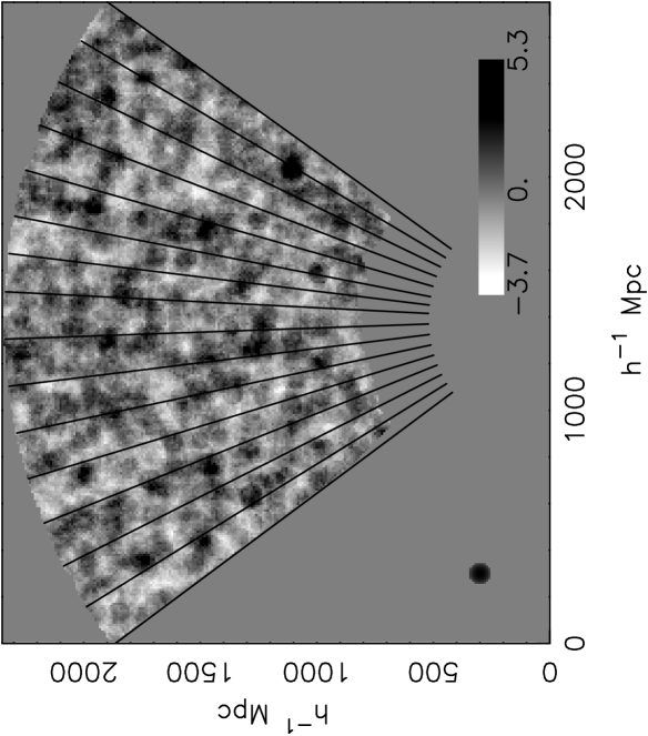
Figure 2: Cuts at constant declination through the smoothed three-dimensional maps of fluctuations in the NGP (upper) and SGP (lower) regions. The x-axis corresponds crudely to the right ascension direction, the y-axis to the redshift direction. The smoothing function is a spherical top hat of diameter 100 h^-1 Mpc as indicated on the lower left of each map. The grey scale is in units of signal-to-noise ratio $S$, as defined in the text, and is the same on both plots. The greyscale bar indicates the maximum and minimum values found in each region. Also shown are the boundaries defined by the right ascension limits of the UKST photographic plates used to construct the survey.

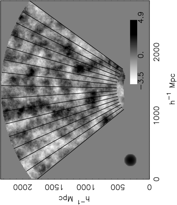
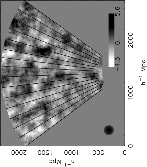
Figure 3: As Fig.2, but with a spherical top hat smoothing function of diameter 200 h^-1 Mpc as indicated on the lower left of each map.

We should perhaps be concerned that errors or uncertainties in the 2QZ selection function may result in spurious creation of fluctuations in Figs 2 & 3. The strongest argument against this possibility are that the selection function and extinction correction have been entirely separated into radial and angular components, and we would expect errors in either component to be manifest as purely radial or angular signals. In Figs 2 & 3 we also show the boundaries defined by the right ascension limits of the UKST photographic plates used to construct the survey. There is no obvious tendency for there to be radial overdensities aligned with these boundaries: although the alignment of a minority of the features appears radial, this is not generally the case, and those features that could be radial in nature may be seen to not fill an entire UKST photographic plate and to extend across the plate boundaries. Overall, we conclude that there are no obvious radial signals associated with the photographic plates. At a greater level of subtlety, there may be variations in the selection function which are not well represented by the assumption of separable components (i.e. angular-dependent variations in the redshift selection function). However, if such effects are present, the existence of under- and over-dense regions apparently at randomly placed redshifts, and not particularly restricted to individual photographic plates, implies that such an effect is not dominating the observed distributions.

Figs 4 & 5 show the same data but now presented as plots of fractional overdensity in QSO number. Because shot noise cannot be neglected, for this exercise we adopt a Bayesian estimator of the fractional overdensity at each location on the map, which maximises the posterior probability

$$P\left(\delta|n_{\rm obs},n_{\rm exp},\sigma^{2}\right)\propto P\left(\delta|\sigma^{2}\right)P\left(n_{\rm obs}|\delta,n_{\rm exp}\right)$$

where $\delta$ is the fractional overdensity and $\sigma^{2}$ is the cosmological variance in $\delta$ on the scale being considered. For Gaussian fluctuations

$$P\left(\delta|\sigma^{2}\right)=\frac{1}{\sqrt{2\pi\sigma^{2}}}\exp{\frac{-\delta^{2}}{2\sigma^{2}}}.$$

The Bayesian estimate has the property that in the presence of random noise the expectation value of a set of points with the same estimated value is the true value, and in that sense it provides the “most likely” value of fluctuation at any point on the map. A maximum likelihood estimate would have the property that the expectation value of a set of points with the same true value is that value. Taking the maximum likelihood estimate in the presence of random noise leads to the statistical distribution of fluctuations being broader than the true distribution, whereas the Bayesian estimator leads to a distribution that is narrower than the true distribution. On the maps presented here, regions of low signal-to-noise have Bayesian estimates of overdensity that are biased towards zero (if a maximum likelihood estimate had been applied instead, regions of low signal-to-noise would appear biased to values more extreme than reality). This effect is noticeable in Figs 4 & 5 at low redshift, where the increasing shot noise leads to some dilution of the measured signal. The Bayesian estimates were created assuming the $\Lambda$CDM model of Section 2.4 with $\sigma_{8}=1.0$.

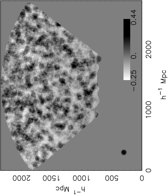
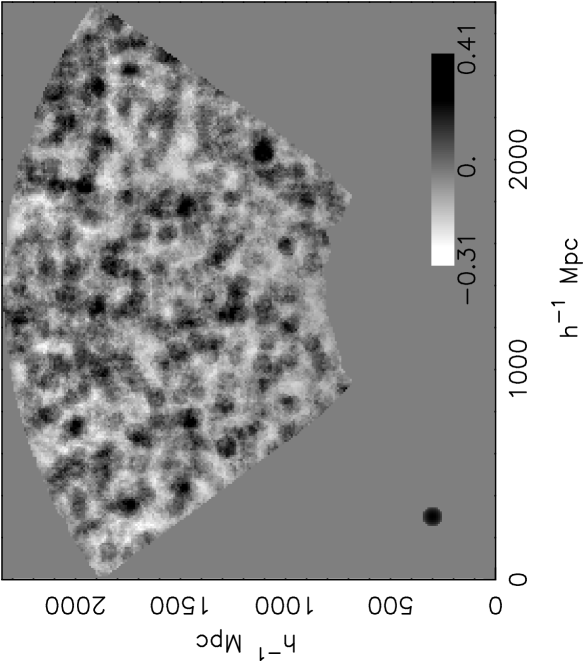
Figure 4: Cuts at constant declination through the Bayesian maps of smoothed fluctuations in the NGP (upper) and SGP (lower) regions. The smoothing function is a spherical top hat of diameter 100 h^-1 Mpc as indicated on the lower left of each map. The grey scale is in units of fractional overdensity and is the same on both plots. The bar also indicates the maximum and minimum values found in each region.

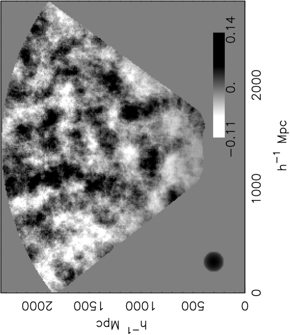
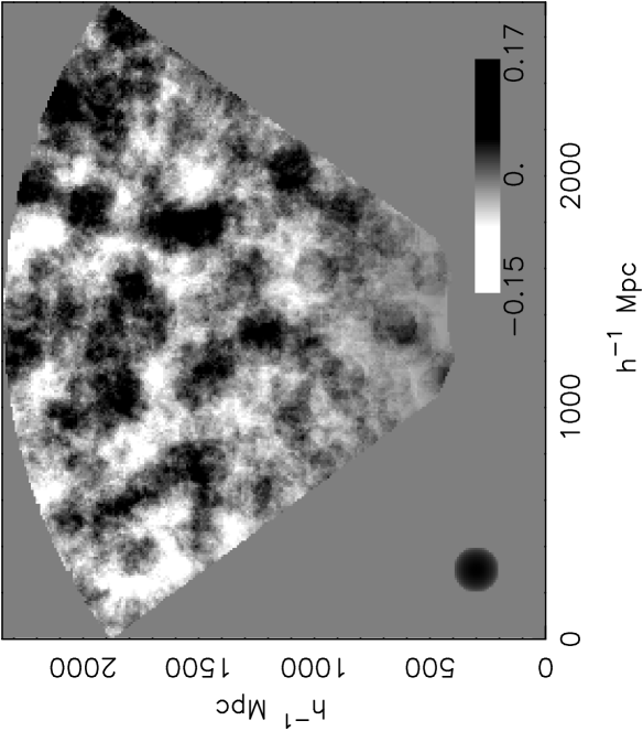
Figure 5: As Fig.4 but with a spherical top hat smoothing function of diameter 200 h^-1 Mpc.

It is immediately seen that the detected fluctuations are all in the linear or weakly non-linear regime, with $-0.31<\delta<0.44$ on scales of 100 h^-1 Mpc and $-0.13<\delta<0.15$ on scales of 200 h^-1 Mpc. Hence the chief result of this section is that large-scale fluctuations in QSO numbers exist, as suspected by previous authors, but unless the bias is much less than unity (the issue of QSO bias is discussed later) the mass density fluctuations are not of sufficiently large amplitude to represent collapsed structures. Hence the best matching hypothesis is that the fluctuations are simply those that are expected in the linear regime of the growth of cosmological structure, and that these are fully represented statistically by the power spectrum of the 2QZ survey (Outram et al., 2003). This hypothesis is tested further in the next section.

2.4 A counts-in-cells analysis

Having demonstrated that statistically-significant fluctuations do exist on large scales, we now should test how these fluctuations compare with the predictions of the cosmological model assuming that on large scales structures are fully represented by the power spectrum. To do this we carry out a counts-in-cells analysis, measuring the sample variance when the data are sampled in independent cubes of a specified size, and comparing that sample variance with the variance expected given a particular choice of power spectrum and normalisation.

The measured cell-to-cell variance has contributions from two sources: cosmological fluctuations and shot noise. Furthermore, because the QSO density varies over the survey, the weight given to each cell should be varied to optimise the signal-to-noise of the overall sample variance. In the limit where QSO numbers are sufficiently large that the shot-noise Poisson distribution tends to a normal distribution, the maximum likelihood estimate of variance of overdensity $\delta$ is

$$s^{2}=\frac{\sum\left(n_{\rm obs}-n_{\rm exp}\right)^{2}-\sum n_{\rm exp}}{\sum n_{\rm exp}^{2}}.$$

As here $n_{\rm exp}>>1$ we adopt this statistic. However, as comparison is made with values of this statistic measured in simulated data (see below) we do not need to assume that the central limit theorem holds. The statistic $s^{2}$ is calculated from the data for cell sizes of 80, 160, 320 & 640 h^-1 Mpc. The use of cubic cells means that, for a given cell size, each cell has shot noise that is statistically independent from its neighbour (although the cosmological signal does not have this property). The variances we expect then are slightly different from the variances that would be calculated using a more standard assumption of spherical cells.

In order to calculate the expected variance for a given cosmological model, we could in principle carry out the standard integration over the power spectrum (e.g. Peacock 1999) assuming an appropriate cell size and shape. There are a number of reasons not to do this, however. First, the surveyed volume does not fill a geometrically simple region, and in fact on the largest scales probed here the survey becomes two-dimensional at low redshifts: the survey dimension in the declination direction is smaller than the largest cell size. This causes the expected variance to have a modified dependence on cell size. Second, the fluctuations in cells of differing sizes are correlated, because the same data are used in the analysis of different cell sizes. The degree of correlation depends on the selection function, the power spectrum, the number of QSOs and the choice of statistic used to measure the variance.

Hence the approach adopted here is to create mock QSO catalogues which have the same selection function and shot noise as the actual data, and in which the expected level of cosmological fluctuations are present, assuming a particular cosmological model. By averaging the values obtained from a large number of such simulations this approach automatically includes the effects of cosmic variance in the distribution of the statistic $s^{2}$. The simulations are generated by creating random density fields on a grid of sampling 10 h^-1 Mpc and size much larger than each region of the 2QZ survey, whose Fourier components are drawn randomly from a normal distribution with variance specified by the power spectrum. The density fields are then multiplied by the 2QZ selection function and extinction corrections. These are Poisson-sampled to create simulated datasets whose properties should mimic in every way the properties of the actual data. This process is repeated for the NGP and SGP regions of the survey.

Figure 6: The variance of counts in cells for the NGP and SGP halves of the survey. Filled points show the measured results after correcting for configuration completeness. Open points show the results after correcting also for spectroscopic completeness. Also shown are mean values and 68 percent confidence intervals derived from the numerical simulations for each region and for each of the two completeness corrections. A value of $\sigma_{8}=1.0$, which best fits the filled points, has been adopted.

The shape of power spectrum adopted is that of Efstathiou et al. (1992). We assume a $\Lambda$CDM cosmology with $\Omega_{\Lambda}=0.7$, $\Omega_{M}=0.3$, $H_{0}=70$ km s^-1 Mpc^-1. To set the normalisation we need to consider the bias of the power spectrum, but dealing with this is complicated by the possibility that departures of the Poisson shot noise from a normal distribution could lead to an offset between the values of the statistic $s^{2}$ measured for the data and for the simulations. Hence we have tested a range of values of the normalisation parameter $\sigma_{8}$ (the rms fluctuation in spheres of diameter 8 h^-1 Mpc), and choose the value which produces the best fit of the statistic $s^{2}$ to the data. The dark matter power spectrum also evolves in amplitude with redshift: what should we assume for the power spectrum of QSO number fluctuations? In fact, we expect QSOs to exhibit larger fluctuations than the dark matter, because QSOs exist in the most massive individual galaxies known (Dunlop et al., 2003), and hence the amplitude of QSO fluctuations will be biased, as described by, e.g. Sheth & Tormen (1999). Because massive galaxies are increasingly rare at higher redshifts, the bias increases with redshift. Hence the expected amplitude of QSO fluctuations should have a redshift dependence which is dependent on the mass of QSO host galaxies. Rather than assuming a theoretical value for the evolution of the bias, we can measure it from the 2QZ survey on smaller physical scales (Croom et al. 2001b, 2004a, 2005, Loaring et al. in prep.) and assume that the cosmological evolution of the bias is the same on large scales as on 10 Mpc scales. To a good approximation, in a $\Lambda$CDM cosmology, the 10 Mpc-scale clustering has an amplitude which is constant with redshift over the range $0.5<z<2$, so here we shall assume that the power-spectrum amplitude is invariant with redshift. The uncertainties in the variance of the cell counts are large, so it should make little difference if in reality there is some departure from the “no-evolution” assumption (in fact, it would be more correct to say that there is strong evolution of the bias which cancels the evolution in the dark matter fluctuations).

Fig. 6 shows the measured variance as a function of cell size for the two halves of the survey. It may be seen that the two halves are in good agreement. Values are shown for both methods of completeness correction: configuration (filled symbols) and spectroscopic (open symbols). Also shown on the figure is the expected variance from the mean of 100 $\Lambda$CDM simulations for a QSO power spectrum normalisation of $\sigma_{8}=1.0$, this being the best fitting redshift-independent power spectrum normalisation. Extrapolated to $z=0$ this would correspond to a bias value $b\simeq 1.1$, but at the typical redshift of the 2QZ sample the bias is substantially higher, consistent with the findings based on measuring the correlation function on smaller scales (Croom et al., 2002, 2004a, 2005). The error bars shown reflect the 68 percent range of values in cell variance obtained from the simulations and are therefore good estimates of the random errors, taking into account both shot noise and cosmic variance. The total $\chi^{2}$ of the fit to both regions is 1.8 with 7 degrees of freedom, assuming the selection function determined from the configuration completeness. The covariance between data points in Fig. 6 is low but is included in the $\chi^{2}$ estimation. The measured variance increases and the best-fitting $\chi^{2}$ value rises slightly to 5.3 if the spectroscopic completeness correction is adopted (open symbols in Fig. 6). It may be seen that on the largest scales the two completeness correction methods reveal systematic uncertainties in the variance that are comparable to the size of the random errors (shot noise and cosmic variance).

If we assume $\sigma_{8}=0$ (i.e. that there are no cosmological fluctuations) $\chi^{2}$ rises to 61, indicating that the hypothesis that the observed fluctuations are merely due to shot noise may be rejected at a significance level of $3\times 10^{-10}$.

We note at this stage that we have not attempted to compare the data with any competing models, but rather simply to test whether the data are consistent with the model favoured by independent cosmological measurements: the approach adopted here may be viewed as being frequentist in nature rather than Bayesian. However, we might wonder whether the shapes and topology of the detected structures are as expected within this model, or whether there is any evidence for significant differences. Statistical tests of topology are beyond the scope of this paper, but by comparing the structures detected on the two scales shown in Figs 2-5, we can see qualitatively at least that there is no evidence for, for example, extremely filamentary structure being responsible for the observed fluctuations on the larger scale. A qualitative comparison of the appearance of Figs 4 & 5 with the $\Lambda$CDM simulated maps (not shown here) also reveals no significant differences.

3 Discussion and conclusions

Fluctuations in QSO space density on scales $\sim 200$ h^-1 Mpc may be seen directly in the QSO distribution (Figs 2-5). It is likely that these fluctuations may be traced out to larger scales, and inspection of the maps and analysis of the variance of the QSO density field indicates the detection of fluctuations on scales possibly as large as 300 h^-1 Mpc. The fluctuations are in good agreement with those expected in a $\Lambda$CDM cosmology with WMAP parameters if we assume that QSO clustering is a biased tracer of dark matter fluctuations, with a bias value that is approximately redshift independent and which is close to the value inferred from QSO clustering on 10 Mpc scales. Since it appears that $b>1$, the fluctuations in mass associated with the observed QSO fluctuations are certainly in the linear or weakly non-linear regime of gravitational collapse, and hence they do not represent collapsed non-linear structures, but are merely a reflection of the large-scale fluctuations expected given the $\Lambda$CDM power spectrum. Figs 2-5 represent direct detection of structure in the distribution of discrete objects on comoving scales that correspond to the scales measured in the cosmic microwave background by WMAP (Spergel et al., 2003).

Consideration of two methods of correcting the measurements for observational selection shows that on the largest scales there may remain systematic variations in survey uniformity at levels that are comparable to the measured fluctuations. For this reason we believe that the 2QZ survey should not be used to attempt to infer more precise values for cosmological parameters such as $\Omega_{M}$ until those systematic non-uniformities can be better corrected for.

One of the most significant features of the results presented here is that there is no evidence for any non-Gaussian initial conditions, which might have been implied had any of the $>50$ Mpc structures previously claimed for QSO distributions turned out to represent collapsed structures. As the counts in cells are completely in accord with the simulations generated from a $\Lambda$CDM power spectrum, we conclude that, as far as this test is concerned, the power spectrum remains a complete description of the large-scale distribution of QSOs.

We have not in this paper attempted to measure the topology of the observed fluctuations. This would be an interesting exercise in order to test whether the observed structures are consistent in every way with the expectations of linearly collapsing structures forming from Gaussian initial conditions.

ACKNOWLEDGEMENTS

The 2dF QSO Redshift Survey was based on observations made with the U.K. Schmidt and Anglo-Australian Telescopes. We thank all the present and former staff of the Anglo-Australian Observatory for their work in building and operating the 2dF facility.

References

- Brand et al. (2003) Brand, K., Rawlings, S., Hill, G.J., Lacy, M., Mitchell, E. & Tufts, J., 2003, MNRAS, 344, 283
- Clowes & Campusano (1991) Clowes, R.G. & Campusano, L.E., 1991, MNRAS, 249, 218
- Crampton et al. (1987) Crampton, D., Cowley, A.P. & Hartwick, F.D.A., 1987, ApJ, 314, 129
- Croom et al. (2001a) Croom, S,M., Smith, R.,J., Boyle, B.J., Shanks, T., Loaring, N.S., Miller, L., & Lewis, I.J., 2001, MNRAS, 322, 29
- Croom et al. (2001b) Croom, S,M., Shanks, T., Boyle, B.J., Smith, R.,J., Miller, L., Loaring, N.S., & Hoyle, F., 2001, MNRAS, 325, 483
- Croom et al. (2002) Croom, S.M., Boyle, B.J., Loaring, N.S., Miller, L., Outram, P.J.; Shanks, T. & Smith, R.J., 2002, MNRAS, 335, 459
- Croom et al. (2004a) Croom, S.M., Boyle, B.J., Shanks, T., Outram, P.J., Smith, R.J., Miller, L., Loaring, N.S., Kenyon, S. & Couch, W., 2004a, in Richards G.T., Hall, P.B., ASP Conf Series Vol. CS-311, AGN Physics with the Sloan Digital Sky Survey, Astron. Soc. Pac., San Francisco
- Croom et al. (2004b) Croom, S.M., Smith, R.J., Boyle, B.J., Shanks, T., Miller, L., Outram, P.J. & Loaring, N.S. 2004b, MNRAS, 349, 1397
- Croom et al. (2005) Croom, S.M., Boyle, B.J., Shanks, T., Smith, R.J., Miller, L., Outram, P.J., Loaring, N.S., Hoyle, F. & Da Angela, J., 2005, MNRAS, 356, 415
- Dunlop et al. (2003) Dunlop, J.S., McLure, R.J., Kukula, M.J., Baum, S.A., O’Dea, C.P. & Hughes, D.H., 2003, MNRAS, 340, 1095
- Efstathiou et al. (1992) Efstathiou, G, Bond. J.R. & White, S.D.M., 1992, MNRAS, 258, 1P
- Floyd et al. (2003) Floyd, D.J.E., Kukula, M.J., Dunlop, J.S., McLure, R.J., Miller, L., Percival, W,J., Baum, S,A. & O’Dea, C.P., 2003, MNRAS, 355, 196
- Kukula et al. (2001) Kukula, M.J., Dunlop, J.S., McLure, R.J., Miller, L., Percival, W,J., Baum, S,A. & O’Dea, C.P., 2001, MNRAS, 326, 1533
- Outram et al. (2003) Outram, P.J. Hoyle, F., Shanks, T., Croom, S.M., Boyle, B.J., Miller, L., Smith, R.J. & Myers, A.D., 2003, MNRAS, 342, 483
- Peacock (1999) Peacock, J.A., “Cosmological Physics”, 1999, Cambridge University Press
- Seldner & Peebles (1978) Seldner, M. & Peebles, P.J.E., 1978, ApJ, 225, 7
- Schlegel et al. (1998) Schlegel, D., Finkbeiner, D. & Davis, M., ApJ, 1998, 500, 525
- Shanks & Boyle (1994) Shanks, T. & Boyle, B.J., 1994, MNRAS, 271, 753
- Sheth & Tormen (1999) Sheth, R.K. & Tormen, G. 1999, MNRAS, 308, 119
- Smith et al. (2004) Smith, R.J. et al., 2004, MNRAS in press
- Spergel et al. (2003) Spergel, D.N., Verde, L., Peiris, H.V., Komatsu, E., Nolta, M.R., Bennett, C.L., Halpern, M., Hinshaw, G., Jarosik, N., Kogut, A., Limon, M., Meyer, S.S., Page, L., Tucker, G.S., Weiland, J.L., Wollack, E. & Wright, E.L., 2003, ApJ Supplement Series, 148, 175
- Webster (1976) Webster, A.S., 1976, MNRAS, 175, 61
- Webster (1982) Webster, A.S., 1982, MNRAS, 199, 683
- Williger et al. (2002) Williger, G.M., Campusano, L.E., Clowes, R.G. & Graham, M.J., 2002, ApJ, 578, 708