The Munich Near–Infrared Cluster Survey (MUNICS) – VI. The stellar masses of K–band selected field galaxies to $z~{}\sim~{}1.2$

Abstract

We present a measurement of the evolution of the stellar mass function in four redshift bins at $0.4<z<1.2$, using a sample of more than 5000 $K$-selected galaxies drawn from the MUNICS (Munich Near-Infrared Cluster Survey) dataset. Our data cover the stellar mass range $10^{10}\leq M/(h^{-2}\,\mathrm{M_{\odot}})\leq 10^{12}$. We derive K–band mass–to–light ratios by fitting a grid of composite stellar population models of varying star formation history, age, and dust extinction to BVRIJK photometry. We discuss the evolution of the average mass–to–light ratio as a function of galaxy stellar mass in the K and B bands. We compare our stellar mass function at $z>0$ to estimates obtained similarly at $z=0$. We find that the mass–to–light ratios in the K–band decline with redshift. This decline is similar for all stellar masses above $10^{10}\,h^{-2}\,\mathrm{M_{\odot}}$. Lower mass galaxies have lower mass–to–light ratios at all redshifts. The stellar mass function evolves significantly to $z=1.2$. The total normalization decreases by a factor of $\sim 2$, the characteristic mass (the knee) shifts toward lower masses, and the bright end therefore steepens with redshift. The amount of number density evolution is a strong function of stellar mass, with more massive systems showing faster evolution than less massive systems. We discuss the total stellar mass density of the universe and compare our results to the values from the literature at both lower and higher redshifts. We find that the stellar mass density at $z\sim 1$ is roughly 50% of the local value. Our results imply that the mass assembly of galaxies continues well after $z\sim 1$. Our data favor a scenario in which the growth of the most massive galaxies is dominated by accretion and merging rather than star formation which plays a larger role in the growth of less massive systems.

1 Introduction

The stellar mass content in galaxies as a function of redshift is one of the most fundamental observables in the quest to understand galaxy formation and evolution. It provides information on the coupling between the growth of structure through the collapse and subsequent merging of dark matter halos and the physical processes governing the evolution of the baryonic matter. Stellar mass in galaxies grows by star formation within galactic disks, as well as by accretion and the merging of galaxies. In fact, these two processes are related, because star formation in disks can be triggered or enhanced by tidal interaction in close encounters and by merging events. This interplay between cosmological structure formation and star formation is believed to govern the mass assembly history of galaxies.

The stellar mass of a galaxy at a given time is difficult to measure, however. While dynamical mass measures are considered to be most reliable, they measure the total mass of an object. The dark matter and gas contributions (which are a function of galaxy type) have to be removed to obtain the stellar mass. These kinds of measurements depend on model assumptions for the dark matter contribution, are observationally very costly, and have therefore only been possible in the local universe so far.

The alternative is to convert the luminosity of a galaxy into a stellar mass by means of a model of its stellar population (derived from photometry or spectroscopy) predicting a mass–to–light ratio ($M/L$) in a certain wavelength band. Near–infrared (NIR) luminosities of galaxies are believed to be well suited for this approach, as the $M/L$values vary only by a factor of roughly 2 across a wide range of star formation histories (SFHs; see, e.g., Rix & Rieke, 1993; Kauffmann & Charlot, 1998; Bell & de Jong, 2001). This compares to a variation of a factor of $\sim 10$ in the B–band. In addition, the optical regime is strongly affected by dust extinction which becomes negligible in the K band for the vast majority of galaxies (Tully et al., 1998). By correlating photometric properties of disk galaxies with inclination, Masters et al. (2003) found the edge–on to face–on extinction correction to be 0.1 mag in the K band.

Measuring the stellar masses of galaxies in the local universe by means of modeling their stellar populations has been re–attempted recently using newly available wide–area galaxy surveys. Kauffmann et al. (2003) used spectroscopic data from the Sloan Digital Sky Survey (SDSS), while Cole et al. (2001) and Bell et al. (2003) combined NIR photometry from the Two Micron All Sky Survey (2MASS) with optical photometry from the 2dF Galaxy Redshift Survey (2dFGRS) and SDSS, respectively, to derive $M/L$values and study the stellar mass function (MF) of galaxies.

At $z>0$, suitable multi–wavelength and redshift data are still sparse. Therefore, the integrated stellar mass density, $\rho_{*}(z)$, has been studied, instead of the stellar MF using the available deep field observations. Dickinson et al. (2003) and Fontana et al. (2003) studied $\rho_{*}(z)$ in the Hubble Deep Fields (HDFs) over the redshift range $0<z<3$ and compared the global integrated SFH of the universe to their measurement of the total stellar mass density. These surveys, however, cover only very small fields (several square arcminutes) and therefore cannot measure the evolution of $\rho_{*}(z)$ below $z\sim 1$. In addition, at higher $z$, cosmic variance, selection biases, and dust extinction are a concern, as the ultraviolet spectral region has redshifted into the observable bands. At $0<z<1$, the total stellar mass density has been estimated from optical and NIR surveys (Brinchmann & Ellis, 2000; Drory et al., 2001a, hereafter MUNICS III; Cohen, 2002), yet the results concerning the evolution of $\rho_{*}(z)$ in this redshift range are still inconclusive. New wide–angle, NIR selected surveys are promising rapid progress (Pozzetti et al., 2003; Firth et al., 2002;Drory et al., 2001b, hereafter MUNICS I) in studying the stellar MF itself instead.

In this work we use data from the wide–field K-band selected field galaxy sample of the MUNICS project (MUNICS I; Feulner et al., 2003, hereafter MUNICS V) to study the stellar MF evolution to $z\sim 1.2$ directly. We derive stellar masses by converting K-band luminosities to mass, by comparing BVRIJK photometry of galaxies to a grid of composite stellar population (CSP) synthesis models based on the simple stellar populations published by Maraston (1998).

We introduce the sample used in this work in Sect. 2 and the method used to derive stellar masses and its uncertainties in Sect. 3. We present the results for the stellar MF in Sect. 4 and discuss the number density of galaxies with $10^{10}\leq M/(h^{-2}\,\mathrm{M_{\odot}})\leq 10^{12}$ in Sect. 5. We present our estimate of the total stellar mass density at $0.4<z<1.2$ and compare it to those in the literature in Sect. 6. Finally, we summarize and discuss our results in Sect.7.

Throughout this work we assume $\Omega_{M}=0.3$, $\Omega_{\Lambda}=0.7$. We write Hubble’s constant as $H_{0}=100\ h\ \mathrm{km\ s^{-1}\ Mpc^{-1}}$, unless noted otherwise. We denote absolute magnitudes in band $X$ by the symbol $M_{X}$ and masses by the symbol $M$.

2 The galaxy sample

MUNICS is a wide–area, medium–deep, photometric and spectroscopic survey selected in the K band, reaching $K\sim 19.5$. It covers an area of roughly one deg² in the K and J bands with optical follow–up imaging in the I, R, V, and B bands in 0.4 deg². MUNICS I discusses the field selection, object extraction, and photometry. Detection biases, completeness, and photometric biases of the MUNICS data are analyzed in detail in Snigula et al. (2002, hereafter MUNICS IV).

The MUNICS photometric survey is complemented by spectroscopic follow–up observations of all galaxies down to $K\leq 17.5$ in 0.25 deg², and a sparsely selected deeper sample down to $K\leq 19$. It contains 593 secured redshifts to date. The spectra cover a wide wavelength range of $4000-8500$Å at $13.2$Å resolution, and sample galaxies at $0<z<1$. These observations are described in detail in MUNICS V.

The galaxy sample used in this work is a subsample of the MUNICS survey Mosaic Fields (see MUNICS I), selected for best photometric homogeneity, good seeing, and similar depth. The subsample covers 0.28 deg² in the B, V, R, I, J, and K bands. It is identical to the sample used in Drory et al. (2003, hereafter MUNICS II) to derive the evolution of the K–band luminosity function (LF). MUNICS II also discusses the procedure used to obtain photometric redshifts for the full sample and the calibration of the technique using spectroscopic redshifts. The reader is referred to this paper for details. The sample used in MUNICS III to derive number densities as a function of mass is selected from the same survey areas but lacks B-band photometry which was added to MUNICS at a later time.

3 Deriving stellar masses

Measuring stellar masses by estimating $M/L$ values in distant galaxies poses some methodological difficulties. At the bright end, even small errors in $M/L$ translate into large errors in the resulting stellar mass, since the LF is very steep. At the faint end, the dynamic range in $M/L$ values increases, and mean stellar ages are harder to derive because of the possibly more complicated SFHs and larger mass fractions of stars born in recent bursts. Therefore, it is important to carefully evaluate the procedure that is used.

In our case, we have photometry in six pass–bands (five colors). Deriving an $M/L$ for each object requires us to estimate a number of parameters similar to the number of observables. We need a photometric redshift (although in MUNICS this is achieved independently of the CSP models used here, it involves the same photometry), an SFH, a mean stellar age, and the amount of dust extinction. These are already four free parameters, and we therefore restrict ourselves to this minimal set of models, leaving out metallicity and superimposed bursts of star formation, instead of including more parameters and marginalizing over them. As noted below, the addition of bursts of star formation has much smaller effects on the NIR $M/L$ values than it has on the optical ones. Since the MUNICS sample contains galaxies more massive than $\sim 10^{10}\mathrm{M_{\odot}}$, it is unlikely that many systems with low metallicity are present in the sample, and we may restrict ourselves to solar metallicity models, especially since the $M/L$ estimates are rather robust with respect to a changes in metallicity around the solar value (see also the discussion of uncertainties in $M/L$ below).

A possible concern might be that we fit spectral energy distributions (SEDs) twice, using one set to derive a photometric redshift and another set to estimate stellar masses, and taht those two sets might not be independent. However, it is important to point out that since we use a much smaller set of semi-empirical SEDs (combining observed SEDs and models) to obtain photometric redshifts, the SEDs used here and those used for the photometric redshifts are, in fact, largely independent. The photometric redshift code uses a set of SEDs that are free combinations of observed galaxy SEDs and model SEDs fitted to combined broad band photometry of objects with spectroscopic redshifts as described in MUNICS II. Hence, they do not allow straight-forward interpretation in terms of physical parameters, such as age or SFH (and, in fact, need not even cover this parameter space in any meaningful way, only the observed colors of galaxies as a function of redshift), and we need an independent grid covering the physical parameter space for the present analysis.

We parameterize the SFH as $\psi(t)\propto\exp(-t/\tau)$,
with $\tau\in\{0.1,0.2,0.4,1.0,2.0,3.0,5.0,8.0,10.0,13.0\}$ Gyr. We extract spectra at 28 ages between 0.001 and 14 Gyr and allow $A_{v}$ to vary between 0 and 3 mag, using a Calzetti et al. (2000) extinction law. The models use solar metallicity and are based on the simple stellar population models by Maraston (1998). We assume a value of 3.33 for the absolute K–band magnitude of the Sun. We use a Salpeter initial mass function (IMF), with lower and upper mass cutoffs of 0.1 and 100 $\mathrm{M_{\odot}}$. This choice of IMF allows us to compare our results to those in the literature more easily. The use of an IMF with a flatter slope at the low mass end will not affect the shape of the MF, it will only change its overall normalization. If, however, the IMF depends on the mode of star formation, e.g. being top–heavy in starbursts, our results will be affected. This particular choice of model grid parameters yields a fairly uniform coverage of color space and represents the SEDs of galaxies in the sample reasonably well in a $\chi^{2}$ sense.

We convert the absolute K–band magnitude, $M_{K}$, into stellar mass by using the K–band mass–to–light ratio, $M/L_{K}$, of the best fitting CSP model in a $\chi^{2}$ sense. We weight by the errors of the photometry and assume an uncertainty of 5% in all model colors to account for the discreteness of the model grid. In addition, another 5% uncertainty is added at J and K wavelengths to account for the intrinsic uncertainty of the models at NIR wavelengths. We employ an age prior falling off as $\exp\{(-\Delta t/1~{}\mathrm{Gyr})^{4}\}$ for ages $\Delta t=t-t_{H}(z)>0$, $t_{H}$ being the age of the universe at redshift $z$, to suppress models with ages greater than the age of the universe at any given redshift.

The value of $M_{K}$ is obtained by taking the restframe K–band magnitude of the best fitting SED of the photometric redshift code of each object (the identical magnitudes were used to construct the LF; see MUNICS II). Since the SED is chosen by a fit using all six pass–bands, the extrapolation to restframe $K$ is based on the same information as an interpolation to restframe $J$ or any other wavelength using this SED would be, and it is therefore no worse. Because NIR SEDs do have some broad features and curvature in the continuum, a simple interpolation between observed magnitudes will not suffice.

The $M/L_{K}$ values of our CSP models as a function of age are shown in Fig. 1. At ages above $\sim 1.5$ Gyr, the variation with age of $M/L_{K}$ is of the order of a factor of $\sim 3$, while the variation between the models at any given age is less than a factor of $\sim 2$. This narrow dynamic range in $M/L$, along with the negligible influence of dust extinction, constitutes the advantage of using the K–band to derive stellar $M/L$ values, making the derived masses quite robust.

We estimate the total systematic uncertainty in the estimated $M/L_{K}$ for each object due to the limited range in parameter space covered by the model grid to be roughly 25% - 30%. In particular, three sources of systematic uncertainty contribute to this number: the effect of neglecting metallicity is found to contribute $\sim 10\%$. We arrive at this number by comparing model $M/L$ values at different ages and metallicities but similar colors, which are compatible with the observations within the photometric errors (the well known age–metallicity degeneracy). This effect is found to be roughly symmetric with respect to metallicity and therefore, if the average metallicity of the galaxies in the current sample is close to the solar value, contributes a close to random uncertainty. The effect of starbursts on top of our smooth SFHs is estimated to change $M/L_{K}$ to lower values by 5% - 10%. This number is obtained by adding bursts of up to 10% in mass and ages of up to 3 Gyr to the $\tau=5$ Gyr and $\tau=10$ Gyr models (assuming no dust extinction; see also Bell & de Jong, 2001 for further discussion of stellar population models of disk galaxy $M/L$ values). Finally, systematic uncertainties in the colors and $M/L_{K}$ values of the underlying stellar population model are estimated to contribute another 5% to 10% uncertainty, especially at younger ages where supergiants contribute a large fraction of the K–band light (see also the discussion of the calibration of these models in Maraston, 1998). The latter would bias the derived $M/L$ to higher values, since the models will tend to underpredict the light contribution of young populations in the NIR.

Another concern lies in the Kron–like aperture photometry that is used in the MUNICS survey to measure total magnitudes. We have performed extensive simulations in MUNICS IV to evaluate the reliability of these total magnitude measurements using an empirical effective surface brightness–size relationship for disk galaxies and the fundamental plane relation for elliptical galaxies.

The main result from this effort is that generally, the magnitudes of $L^{*}$ objects are fairly well recovered. Pure exponential profiles suffer only very little bias and almost no magnitude dependent trend over a wide range of luminosities, even at the highest redshift we probe here. In contrast, de Vaucouleurs profiles show higher lost–light fractions at bright intrinsic magnitudes of $L\geq L^{*}+1$ and a strong magnitude dependent increase of the lost–light fraction with increasing intrinsic magnitude. This is due to the fact that brighter elliptical galaxies have lower mean surface brightness.

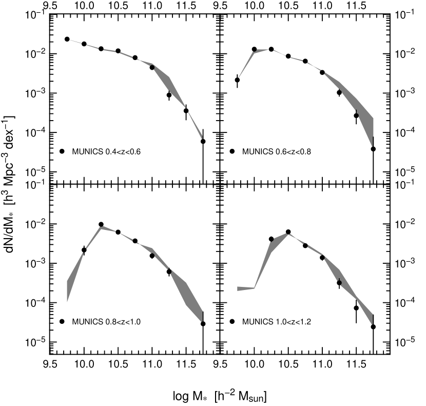
Figure 2: The effect of correcting for the lost–light fraction in Kron–like magnitudes at high redshift. The solid dots represent the raw uncorrected data, the dashed region shows the lost–light correction according to simulations in MUNICS IV. The region is bounded by using face on exponential disks and pure de Vaucouleurs profiles (see text).

We cannot correct for this effect without assuming a morphological mix of galaxies as a function of redshift or being able to reliably measure bulge–to–disk ratios in our sample. Therefore, we calculate the effect it has on our MFs, by assuming first that all galaxies are exponential disks and second that all galaxies have de Vaucouleurs profiles, and show the MFs for both cases in Fig. 2. The data points represent the uncorrected MF and the shaded area the range of possible values between the two cases.

Note that the assumption that all galaxies follow de Vaucouleurs profiles does represent an upper limit, since the lost–light fraction in this case is higher than in any other. The case in which all galaxies are assumed to follow exponential profiles does not represent a lower limit, however. Because of its dependence on intrinsic magnitude, the effect on the MF is most notable at the massive end but does not dominate the uncertainty there (these bins typically have fewer than five objects, and the brightest bin has one object; see the discussion of uncertainties below). Furthermore, around the knee of the MF (at the characteristic mass $M^{*}$), this correction appears irrelevant, as the intrinsic magnitudes there are well recovered. It also seems that the shape of the MF is altered only very little. Finally, the reader might note that in some cases at the (incomplete) faint end (e.g., at $z=1.1$ and $\log M=10.25$) the corrected range extends below the uncorrected data. This is an artifact caused by the incomplete data at lower masses and by binning. Objects in a bin are corrected toward higher masses (and move out of the bin), while too few objects are corrected into the bin from below (because of strong incompleteness). The bin therefore effectively loses objects.

4 The stellar mass function

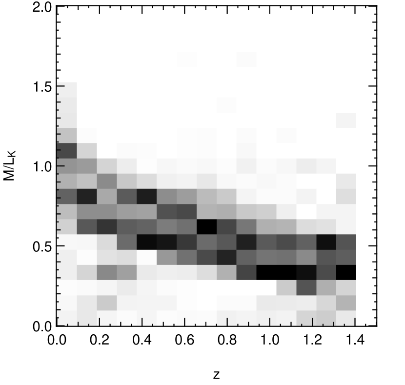
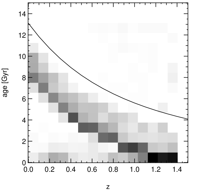
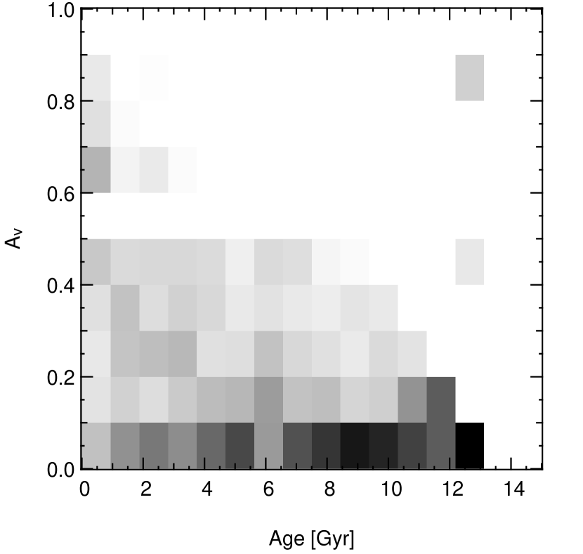
Figure 3: Distributions of model parameters that we obtain by fitting BVRIJK multicolor data to the CSP model grid. The left–hand panel shows the distribution of the K–band $M/L$ values with redshift. The middle panel the distribution of mean luminosity weighted stellar age as a function of redshift, the age of the universe using $h=0.72$ is plotted as a reference (solid line). The right hand panel shows the distribution of the the dust extinction coefficient $A_{V}$ vs. the luminosity weighted mean age.

The distributions of model parameters that we obtain by fitting the data to the CSP model grid described above are shown in Fig. 3. The left–hand panel shows the distribution of the K–band $M/L$ values with redshift. The middle panel shows the distribution of mean luminosity weighted stellar age as a function of redshift. The age of the universe is plotted as a reference (solid line), using $h=0.72$. The right hand panel shows the distribution of the dust extinction coefficient $A_{V}$ versus the luminosity weighted mean stellar age. The average $V_{\mathrm{max}}$–weighted K–band $M/L$ values in our four redshift bins are given in Table 1 and plotted in Fig. 4. Table 1 also lists the average B–band $M/L$ values for comparison to other work.

At $z\sim 0$, the mean luminosity weighted stellar age is 8.1 Gyr with a mean $M/L_{K}$ of 0.91. Most objects have $M/L_{K}$ between 0.7 and 1.2 and the majority have moderate dust extinction of $A_{V}<0.6$. Note that the absolute value of $M/L_{K}$ is not only IMF–dependent but also depends on the specific stellar population synthesis model used (because of the differing treatment of stellar remnants) and should therefore be taken with caution. Instead, we concentrate on the relative change of $M/L_{K}$  and therefore the relative change of the MF, with $z$.

Star formation in our $K$-selected objects begins well before $z\sim 1.5$. The bulk of the stars in the local universe is therefore older than 8 Gyr and formed before $z=1$, consistent with recent estimates of the total stellar mass density of the universe, which suggest that the stellar mass density at $z\sim 1$ is roughly half its local value (see also Sect. 6; Dickinson et al., 2003; Fontana et al., 2003; Cole et al., 2001). Only very few objects at low redshift have $M/L_{K}<0.5$ and therefore mean ages less than $\sim 3$ Gyr (see Fig. 1). This is no surprise in a K–band selected survey with a magnitude limit of $K<19.5$. There are very few objects (well below 1% of the sample) that scatter to ages above the age of the universe despite the age prior included in the likelihood function. Inspection of those objects shows that they are most likely photometrically problematic objects (blended objects; objects with strong emission lines; objects affected by bright star artifacts; extended low–$z$ objects with an overlapping foreground star). The large majority of objetcts, however, yields acceptable ($\chi^{2}<10$) fits to the model grid.

As expected, the range of $M/L$ values evolves steadily toward lower averages with increasing redshift as the stars inevitably become younger. No population of very young objects with ages of $\sim 1$ Gyr is found at $z<1$, although there might be such populations at magnitudes below our detection limit of $K<19.5$ and hence stellar masses below $\sim 10^{10}$ $h^{-2}\,\mathrm{M_{\odot}}$ at lower redshift. This again indicates that the objects in our sample experienced their most intensive phase of star formation at redshifts above $z\sim 1.5$. Indeed, closer to the redshift limit of the current analysis at $z=1.2$, objects with ages of around 1 Gyr do appear, while older objects with ages of 3 Gyr are still present up to the survey’s redshift limit. This indicates that we approach the epoch of the formation of some of these systems although we do not quite reach it with MUNICS. The presence of apparently old and massive stellar systems at $z\sim 1$ has also been pointed out recently by several authors studying spectroscopic samples of extremely red objects (EROs), e.g., by the K20 survey (Cimatti et al., 2002) using deep optical spectroscopy, and by Saracco et al. (2003), by spectroscopic followup of MUNICS–selected EROs in the NIR. It will be very interesting to see the results from larger and deeper surveys targeted at galaxies in the redshift range $1<z<2$.

As is observed in the local universe, lower mass galaxies have on average lower $M/L$ values at all redshifts in our sample. This is shown in Fig. 4 and Table 1. We wish to point out, however, that the evolution of $M/L_{K}$ with redshift seems quite independent of galaxy stellar mass. If anything, more massive systems show a slightly flatter evolution. In addition, older systems have lower dust extinction, and there are no strongly dust reddened objects with $A_{V}>1$ in the sample.

Finally, we construct the stellar MF, using the $V_{\mathrm{max}}$ method to account for the fact that fainter galaxies are not visible in the whole survey volume. Here each galaxy in a given redshift bin $[z_{l},z_{h})$ contributes to the number density an amount inversely proportional to the volume in which the galaxy is detectable in this redshift bin. The method is fully analogous to the one used for the LF in MUNICS II, and the reader is referred to that work for details.

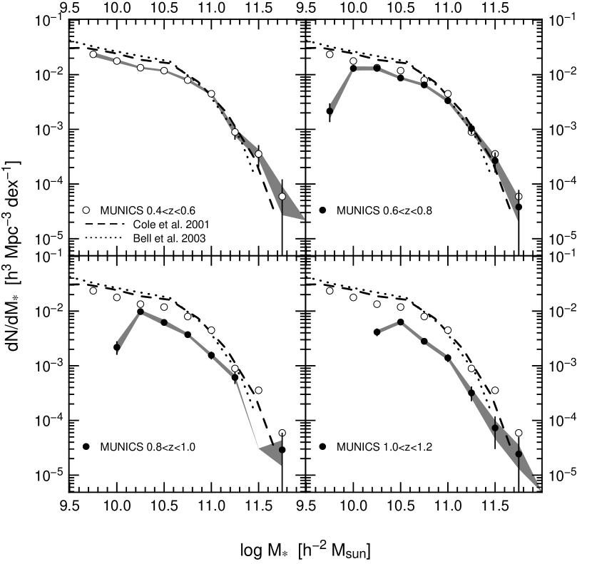
Figure 5: The evolution of the stellar MF with redshift. The open symbols are the MUNICS values at $0.4<z<0.6$, the closed symbols are the MUNICS values at higher redshifts. The lowest $z$ values are shown in all panels for comparison. Error bars denote the uncertainty due to Poisson statistics. The shaded areas show the 1 $\sigma$ range of variation in the MF given the total systematic uncertainty in $M/L_{K}$ discussed in Sect. 3. The dotted and dashed lines show the $z=0$ stellar MF derived similarly to our methods using SDSS, 2dF, and 2MASS data (Bell et al., 2003; Cole et al., 2001).

Fig. 5 shows the MF of galaxies with $10^{10}<M/(h^{-2}\,\mathrm{M_{\odot}})<10^{12}$ in four redshift bins centered at $z=0.5$, $z=0.7$, $z=0.9$, and $z=1.1$. The results for the local stellar MF from Cole et al. (2001) and Bell et al. (2003), derived by fitting stellar population models to multicolor photometry and deriving NIR $M/L$ values similarly to the method employed here are also shown for comparison as a dashed and a dotted line, respectively. The curve from Bell et al. (2003) has been corrected to a 30% higher normalization to account for their choice of IMF, which is a Salpeter form with a lower fraction of low mass stars (“diet”-IMF) that yields 30% lower masses. The data from the lowest redshift bin, $0.4<z<0.6$, are shown alongside the higher–redshift data, for easier comparison, as open symbols. Error bars denote the uncertainty due to Poisson statistics. The shaded areas show the 1 $\sigma$ range of variation in the MF from Monte–Carlo simulations given the total systematic uncertainty in $M/L_{K}$ of 30% discussed in Sect. 3, assuming a Gaussian distribution. Although this is not strictly realistic, we note that systematic uncertainties discussed above are not dominated by any one particular asymmetric bias. The lost–light effect is not included in these simulations. The values of our MFs are given in Table 2, along with the errors from Poisson statistics and the systematic uncertainties in $M/L_{K}$. This table also quotes the values we obtain assuming that all galaxies follow an $r^{1/4}$ light profile, this case being the one with the largest corrections to the Kron–like photometry.

We stress the fact that the highest mass bin, at $\log M/(h^{-2}\,\mathrm{M_{\odot}})=11.75$, typically contains only one object and the next bin, at $\log M/(h^{-2}\,\mathrm{M_{\odot}})=11.5$, typically contains fewer than five objects. Hence, moving objects from one bin to the other at the very bright end (either through the uncertainty in $M/L_{K}$ or through lost–light corrections to the photometry) has a big effect. Furthermore, the MF is steepest here, so a small change to the luminosity has a big effect on the derived mass. Therefore, the uncertainties at the very bright end are much larger than those around the knee of the MF (around the characteristic mass, $M^{*}$, where bins contain typically $\sim 200$ objects). The mass bin $\log M/(h^{-2}\,\mathrm{M_{\odot}})=11.5$ at z=0.9 contains no objects, and therefore the uncertainty contours are artificially compressed there. At the very bright end, the Poisson errors dominate our total uncertainty in the MF. Shot noise and $M/L_{K}$ systematics contribute equally at the knee around $M^{*}$. The lost–light uncertainties are smaller than the shot noise and the systematics associated with assigning $M/L_{K}$.

The lowest redshift bin shows remarkable agreement with the $z=0$ values, despite the different selection at low versus high redshift and the different model grids used, although we obtain slightly lower number densities at $\log M/(h^{-2}\,\mathrm{M_{\odot}})\leq 10.5$. Therefore, there seems to be not much evolution in stellar mass at $z<0.5$. The general trend at higher redshift is for the total normalization of the stellar MF to go down and for the knee to move toward lower masses. This causes the higher masses to evolve faster in number density than lower masses, is well visible in Fig. 5 at $10.5<\log M/(h^{-2}\,\mathrm{M_{\odot}})<11.5$ and is further discussed in Sect. 5.

These results have to be seen in the context of the evolution of the K–band LF (MUNICS II, using the same sample as in this work; also Pozzetti et al., 2003; Firth et al., 2002). It is important to stress that the results obtained here depend strongly on the quality of the underlying LF. The trends with mass observed here depend on the exact shape of the LF around the characteristic luminosity, $L^{*}$, and its evolution with $z$. Since the relative change in $M/L_{K}$ is similar at all masses (Fig. 4), the increase in number density evolution with mass can be explained in the following way: as one is moving to higher masses (at any given $M/L_{K}$), the corresponding luminosity is moving down the steepening part of the LF, so that the same relative change in $M/L_{K}$ yields a higher change in the number density at a higher stellar mass. This is a very fundamental observation and it is hard to see how this can be avoided.

5 The number density of massive systems

In this section we concentrate on the number density of galaxies having stellar masses exceeding some mass limits, in other words, the integrated stellar MF. Although this information is already implicitly contained in Fig. 5, its integrated form is less noisy and has been frequently discussed in recent literature (e.g. MUNICS III; Im et al., 1996; Kauffmann et al., 1996; Driver et al., 1998; Totani & Yoshii, 1998; Kauffmann & Charlot, 1998; Fontana et al., 1999; Firth et al., 2002; Cohen, 2002).

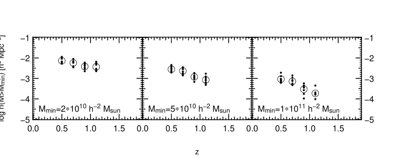
Figure 6: Co-moving number density of objects having stellar masses exceeding $M_{\mathrm{lim}}=2\times 10^{10}\,h^{-2}\,\mathrm{M_{\odot}}$, $M_{\mathrm{lim}}=5\times 10^{10}\,h^{-2}\,\mathrm{M_{\odot}}$, and $M_{\mathrm{lim}}=1\times 10^{11}\,h^{-2}\,\mathrm{M_{\odot}}$ The solid points denote the values measured separately in each survey field, the open circles denote the mean values over the whole survey area. values.

We present the results in the same fashion that was used in MUNICS III, where we used the assumption that all stars form at $z=\infty$ to maximize the stellar mass at any K–band luminosity. We plot the number density of systems more massive than a given mass $M_{\mathrm{lim}}$. We use $M_{\mathrm{lim}}=2\times 10^{10}\,h^{-2}\,\mathrm{M_{\odot}}$, $M_{\mathrm{lim}}=5\times 10^{10}\,h^{-2}\,\mathrm{M_{\odot}}$, and $M_{\mathrm{lim}}=1\times 10^{11}\,h^{-2}\,\mathrm{M_{\odot}}$. The results are shown in Fig. 6 and listed in Table 3.

Again, it is clearly visible that objects with higher stellar masses show stronger evolution in number density, a result that we have already seen in the stellar MF in Sect. 4. The number density of objects more massive than $2\times 10^{10}\,h^{-2}\,\mathrm{M_{\odot}}$ declines by a factor of $\sim 2$ to $z\sim 1$, again pointing to half the stellar mass having formed since $z\sim 1$ (see discussion below). For objects having $M>5\times 10^{10}\,h^{-2}\,\mathrm{M_{\odot}}$, the decline is by a factor of 3.3. Objects with $M>10^{11}\,h^{-2}\,\mathrm{M_{\odot}}$ evolve by a factor of 4.9 in number density. If we stretch all sources of uncertainty to their maximum, including the lost–light corrections, this number changes to a factor of 2.7. For stellar masses below $10^{11}\,h^{-2}\,\mathrm{M_{\odot}}$, the uncertainties play a much smaller role.

We use Fig. 6 to make another point concerning cosmic variance. The figure shows the average number densities in our survey, but also the individual numbers from eight disjoint survey patches, each approximately 130 arcmin² in size (see MUNICS II). There is considerable variance among the survey fields even for the lowest mass limit where the number of objects is largest. It is also apparent, that the variance increases rapidly toward higher limiting mass, not only because of smaller numbers, but also because of the higher clustering of massive galaxies (e.g. Daddi et al., 2000; Norberg et al., 2001; Madgwick et al., 2003).

6 The total stellar mass density

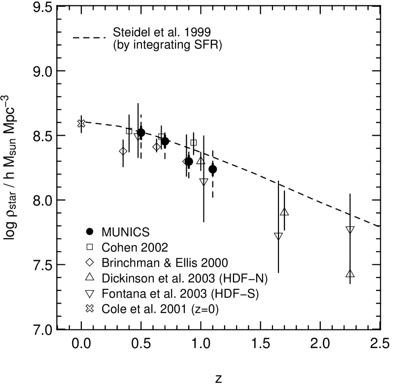
Figure 7: The evolution of the total stellar mass density in the universe. The closed circles are the MUNICS values, open symbols are values from the literature. The integrated star formation rate (dashed curve) is shown for comparison. The thick error bars on the MUNICS values (solid dots) are the statistical errors associated with the data. The dashed error bars show the variance we get from the MUNICS data in GOODS size patches.

The total stellar mass density of the universe, observationally the complement of the SFH of the universe (e.g., Madau et al., 1996; Steidel et al., 1999), is shown in Fig. 7. We also plot the local value from Cole et al. (2001), values from the HDFs (Dickinson et al., 2003; Fontana et al., 2003) covering $z>1$, and values from Cohen (2002) and Brinchmann & Ellis (2000) at $z<1$. Additionally, we integrate the SFH curve (including extinction correction) from Steidel et al. (1999) for comparison. We also list the results in Table 4.

At $z>=0.9$ we do not sample the stellar MF to low enough masses to be able to compute the necessary integral without corrections. We therefore assume that the faint end slope does not change with redshift, using the faint end slope of a Schechter fit to our $z=0.5$ data normalized to the higher redshift MFs to compute corrections to the total stellar mass. This correction is a factor of 1.35 in the highest redshift bin.

The results from these different surveys agree reasonably well, given their differing selection techniques and methodologies. While Brinchmann & Ellis (2000) used a small (321 objects) sample and a method similar to ours to derive $M/L_{K}$  Cohen (2002) uses galaxy SED evolutionary models (assigning fixed SFHs and formation redshifts to $z=0$ galaxy types) to read off the change in $M/L_{K}$ with $z$. This is then used to convert K–band luminosity densities to stellar mass densities, assuming $M/L_{K}\ =0.8$ for all galaxy types locally. This method typically yields higher $M/L$ values than actual SED fitting where the star formation rate and mean age at each redshift are essentially free parameters and are allowed to produce younger objects as needed. We can compare our average B–band $M/L$ to the numbers obtained by Dickinson et al. (2003). They quote average $M/L_{B}$ values in the redshift range 0.5 – 1.4 between 0.96 and 1.38 depending on the model (number of components and metallicity) which compares well to our average values from Table 1. The average $M/L_{B}$ for our whole sample is 1.28.

From our data it appears that 50% of the local mass in stars has formed since $z\sim 1$. This is consistent with results obtained in the HDFs (Dickinson et al., 2003; Fontana et al., 2003; Rudnick et al., 2003), although the volume probed by the HDFs at $z<1$ is very small and the results therefore uncertain at these redshifts. The results for the integrated star formation rate of the universe traced by the UV continuum emission agree with our results as well as the HDF results, reasonably well. The data from Brinchmann & Ellis (2000) are consistent with ours at $z\sim 1$ but are lower at $z\sim 0.4$ and seem to under–predict the local value if extrapolated. The values obtained by Cohen (2002) are higher at $z\sim 1$, which we think is attributable to their method of deriving $M/L_{K}$.

It is worth noting that the results from the HDF–N differ by a factor $\sim 2$ from the HDF–S results, which is attributable to cosmic variance. The MUNICS values in Fig. 7 are shown with their statistical errors (thick error bars), which amount to roughly 10%. We also show the variance we get in our sample divided into GOODS size patches of 150 arcmin² (dashed error bars), showing that at these redshifts, even surveys like GOODS (Great Observatories Origins Deep Survey) are expected to be dominated by cosmic variance. We expect differences of around 50% between the two GOODS areas.

7 Discussion and conclusions

The results of this study of the evolution of stellar masses of galaxies to $z=1.2$ can be summarized as follows.

1. The mass–to–light ratios ($M/L$s) in the K–band decline with redshift by similar amounts for all stellar masses above $10^{10}\,h^{-2}\,\mathrm{M_{\odot}}$. Lower mass galaxies have lower $M/L$ values at all redshifts.

2. The stellar mass function evolves significantly to $z=1.2$. The total normalization decreases by a factor of $\sim 2$, the characteristic mass (the knee) shifts towards lower masses and the bright end therefore steepens with redshift.

3. The amount of number density evolution is a strong function of stellar mass. More massive systems show stronger evolution in their number density.

4. In total, roughly half the stellar mass in the present day universe forms at $0<z<1$.

At first sight these results seem to disagree with recent measurements of the number density of morphologically selected or color–selected (extremely red objects, or EROs) early–type systems (Im et al., 1996; Schade et al., 1999; Moriondo et al., 2000; Daddi et al., 2000; but see also Treu & Stiavelli, 1999; Menanteau et al., 1999). However, our sample is K–band flux limited and therefore largely morphologically blind. The statement that the number densities of galaxies as a function of their stellar mass content evolves does not contradict a constant number density of elliptical galaxies, as long as their morphologies do not change (on average) as their stellar mass grows. Early type galaxies in clusters, however, show clear evidence for passive evolution, at least up to $z\sim 1$ (e.g., Bender et al., 1996; Ziegler & Bender, 1997; Stanford et al., 1998; Kelson et al., 2000, 2001; van Dokkum & Franx, 2001; van Dokkum & Stanford, 2003) which implies a constant stellar mass. In the field (van Dokkum et al., 2001; Treu et al., 2001), early–type galaxies seem to show larger age scatter, and in a recent study of a sample of strong gravitational lens galaxies, van de Ven et al. (2003) found that about half of the field elliptical galaxies have younger stellar populations and are best fitted by formation redshifts extending down to $z_{f}\sim 1$, a scenario that is fully compatible with our results.

Furthermore, we still find that more massive galaxies have older luminosity weighted mean ages (higher $M/L$) and that while galaxies with young populations are present in larger numbers at $z\sim 1$, almost maximally old systems are still present even at the highest redshift we probe. This has also been demonstrated by spectroscopic studies of samples of EROs, most recently by the K20 survey (Cimatti et al., 2002), using deep optical spectroscopy, and by Saracco et al. (2003), using spectroscopic follow-up of MUNICS–selected EROs in the NIR.

While half the present day stellar mass seems to form after $z\sim 1$, it seems that the oldest stellar populations at each epoch are harbored by the most massive objects. The growth of stellar mass at the high mass end of the stellar MF is driven by accretion and merging of objects having similarly old populations, rather than by star formation. This must be the case because if star formation were to contribute equally to the growth of stellar mass at all masses, the ratio of young to old stars, and hence $M/L$, would be the same in all galaxies, which is not the case. The higher $M/L$ of the more massive galaxies indicates that star formation since $z\sim 1$ is not as important in these objects as it is at lower masses. A similar result in the local universe was shown by Kennicutt et al. (1994), and Brinchmann & Ellis (2000) explicitly arrived at the same conclusion by looking at the star formation rate per unit stellar mass in their high-$z$ sample.

To account for their rapid change in number density, however, merging and accretion have to dominate. Indeed, Conselice et al. (2003) find that in the HDF, the merger fraction of massive galaxies increases more rapidly than that of less massive galaxies. Another argument in support of this picture has been put forward by Cowie et al. (1996). By combining K–band imaging and star formation measurements from OII equivalent widths, they showed that the star formation rate per unit K band luminosity (as a surrogate for stellar mass) is lower in higher mass systems and that this quantity increases with redshift, the increase being slower for higher mass systems (i.e., they formed earlier). In addition, many authors noted a steep increase in the star formation rate at $0<z<1$, (e.g., Lilly et al., 1996; Hammer et al., 1997; Rowan-Robinson et al., 1997; Flores et al., 1999).

We wish to point out that the observed trend in density evolution as a function of mass is qualitatively consistent with the expectation from hierarchical galaxy formation models. The most rapid evolution is predicted for the number density of the most massive galaxies, while the number density of less massive galaxies is predicted to evolve less. While older models tended to over–predict this evolution, more recent models seem to yield results more consistent with the redshift distribution of K–band selected galaxies (Fontana et al., 1999; Firth et al., 2002). A detailed comparison of the predicted stellar MFs and colors of galaxies with these observations has yet to be done.

Upcoming large area surveys will advance this field significantly by providing more colors, morphological information, and spectroscopic information. This will allow us to use better CSP model grids, divide the samples up by morphology, and include direct star formation measurements from spectroscopy. This will allow us to determine the relative contributions of star formation and accretion/merging to the mass build–up as a function of cosmic epoch and galaxy properties. Hence these datasets will provide a much more complete picture of the assembly process of galaxies.

Figure 1: K–band $M/L$ value as a function of age of the CSP models that we use. Lines from top to bottom show $M/L_{K}$ of star formation histories of the form $\psi(t)\propto\exp(-t/\tau)$, with $\tau\in\{0.1,0.2,0.4,1.0,2.0,3.0,5.0,8.0,10.0,13.0\}$.

Figure 4: The average K–band $M/L$ value as a function of stellar mass and redshift.

Table 1: Average K–band and B–band $M/L$ value as a function of redshift.

$z$	$2\times 10^{10}<M/(h^{-2}\,\mathrm{M_{\odot}})<5\times 10^{10}$		$5\times 10^{10}<M/(h^{-2}\,\mathrm{M_{\odot}})<1\times 10^{11}$		$M/(h^{-2}\,\mathrm{M_{\odot}})>1\times 10^{11}$
	$\langle M/L_{K}\ \rangle$	$\langle M/L_{B}\ \rangle$	$\langle M/L_{K}\ \rangle$	$\langle M/L_{B}\ \rangle$	$\langle M/L_{K}\ \rangle$	$\langle M/L_{B}\ \rangle$
0.5	0.65	1.69	0.71	2.18	0.74	2.58
0.7	0.58	1.36	0.64	1.88	0.68	2.27
0.9	0.46	0.61	0.55	1.26	0.62	1.83
1.1	0.35	0.23	0.43	0.49	0.55	1.23

Table 2: The values of the stellar mass function in 4 redshift bins.

$z$	$\log M$	$dN/dM$	$\pm$$\sqrt{(}N)$ $\pm$$M/L_{K}$	max ($r^{1/4}$)	$z$	$\log M$	$dN/dM$	$\pm$$\sqrt{(}N)$ $\pm$$M/L_{K}$	max ($r^{1/4}$)
	$h^{-2}\,\mathrm{M_{\odot}}$	$h^{3}~{}\mathrm{Mpc}^{-3}$	$h^{3}~{}\mathrm{Mpc}^{-3}$	$h^{3}~{}\mathrm{Mpc}^{-3}$		$h^{-2}\,\mathrm{M_{\odot}}$	$h^{3}~{}\mathrm{Mpc}^{-3}$	$h^{3}~{}\mathrm{Mpc}^{-3}$	$h^{3}~{}\mathrm{Mpc}^{-3}$
0.5	9.75	2.35$\times 10^{-2}$	($\pm$2.29$\pm$2.07)$\times 10^{-3}$	2.34$\times 10^{-2}$	0.7	9.75	$\cdots$	$\cdots$	$\cdots$
	10.00	1.78$\times 10^{-2}$	($\pm$1.27$\pm$1.24)$\times 10^{-3}$	1.74$\times 10^{-2}$		10.00	1.32$\times 10^{-2}$	($\pm$1.46$\pm$1.08)$\times 10^{-3}$	1.02$\times 10^{-2}$
	10.25	1.34$\times 10^{-2}$	($\pm$9.06$\pm$5.36)$\times 10^{-4}$	1.26$\times 10^{-2}$		10.25	1.30$\times 10^{-2}$	($\pm$0.88$\pm$1.06)$\times 10^{-3}$	1.34$\times 10^{-2}$
	10.50	1.18$\times 10^{-2}$	($\pm$8.43$\pm$4.80)$\times 10^{-4}$	1.06$\times 10^{-2}$		10.50	8.68$\times 10^{-3}$	($\pm$5.91$\pm$4.56)$\times 10^{-4}$	8.17$\times 10^{-3}$
	10.75	7.95$\times 10^{-3}$	($\pm$6.90$\pm$4.77)$\times 10^{-4}$	7.31$\times 10^{-3}$		10.75	6.49$\times 10^{-3}$	($\pm$5.01$\pm$3.94)$\times 10^{-4}$	6.16$\times 10^{-3}$
	11.00	4.47$\times 10^{-3}$	($\pm$5.17$\pm$2.94)$\times 10^{-4}$	5.61$\times 10^{-3}$		11.00	3.35$\times 10^{-3}$	($\pm$3.59$\pm$2.51)$\times 10^{-4}$	3.70$\times 10^{-3}$
	11.25	8.92$\times 10^{-4}$	($\pm$2.30$\pm$1.48)$\times 10^{-4}$	2.56$\times 10^{-3}$		11.25	1.03$\times 10^{-3}$	($\pm$1.99$\pm$1.38)$\times 10^{-4}$	1.92$\times 10^{-3}$
	11.50	3.55$\times 10^{-4}$	($\pm$1.45$\pm$0.72)$\times 10^{-4}$	4.15$\times 10^{-4}$		11.50	2.67$\times 10^{-4}$	($\pm$1.01$\pm$0.67)$\times 10^{-4}$	7.27$\times 10^{-4}$
	11.75	5.92$\times 10^{-5}$	($\pm$5.92$\pm$3.21)$\times 10^{-5}$	5.92$\times 10^{-5}$		11.75	3.80$\times 10^{-5}$	($\pm$3.80$\pm$1.84)$\times 10^{-5}$	2.29$\times 10^{-4}$
0.9	10.25	9.76$\times 10^{-3}$	($\pm$9.39$\pm$7.66)$\times 10^{-4}$	7.39$\times 10^{-3}$	1.1	10.25	$\cdots$	$\cdots$	$\cdots$
	10.50	6.19$\times 10^{-3}$	($\pm$5.24$\pm$7.12)$\times 10^{-4}$	6.17$\times 10^{-3}$		10.50	6.23$\times 10^{-3}$	($\pm$5.61$\pm$4.51)$\times 10^{-4}$	5.40$\times 10^{-3}$
	10.75	3.71$\times 10^{-3}$	($\pm$3.32$\pm$2.26)$\times 10^{-4}$	3.31$\times 10^{-3}$		10.75	2.80$\times 10^{-3}$	($\pm$2.80$\pm$2.53)$\times 10^{-4}$	3.24$\times 10^{-3}$
	11.00	1.55$\times 10^{-3}$	($\pm$2.14$\pm$1.33)$\times 10^{-4}$	2.41$\times 10^{-3}$		11.00	1.39$\times 10^{-3}$	($\pm$1.88$\pm$1.20)$\times 10^{-4}$	1.72$\times 10^{-3}$
	11.25	6.12$\times 10^{-4}$	($\pm$1.34$\pm$0.64)$\times 10^{-4}$	7.59$\times 10^{-4}$		11.25	3.19$\times 10^{-4}$	($\pm$8.86$\pm$6.55)$\times 10^{-5}$	6.87$\times 10^{-4}$
	11.50	$\cdots$	$\cdots$	3.21$\times 10^{-4}$		11.50	7.31$\times 10^{-5}$	($\pm$4.22$\pm$2.70)$\times 10^{-5}$	1.46$\times 10^{-4}$
	11.75	2.90$\times 10^{-5}$	($\pm$2.90$\pm$1.45)$\times 10^{-5}$	5.79$\times 10^{-5}$		11.75	2.43$\times 10^{-5}$	($\pm$2.43$\pm$1.13)$\times 10^{-5}$	4.91$\times 10^{-5}$

Table 3: Number density of objects with stellar mass $M>M_{\mathrm{lim}}$.

$z$	$n(M>2\times 10^{10}\,h^{-2}\,\mathrm{M_{\odot}})$	$n(M>5\times 10^{10}\,h^{-2}\,\mathrm{M_{\odot}})$	$n(M>1\times 10^{11}\,h^{-2}\,\mathrm{M_{\odot}})$
	$h^{3}\,\mathrm{Mpc}^{-3}$	$h^{3}\,\mathrm{Mpc}^{-3}$	$h^{3}\,\mathrm{Mpc}^{-3}$
0.5	(7.37$\pm$0.95)$\times 10^{-03}$	(2.82$\pm$0.59)$\times 10^{-03}$	(9.22$\pm$3.38)$\times 10^{-04}$
0.7	(5.76$\pm$0.68)$\times 10^{-03}$	(2.32$\pm$0.43)$\times 10^{-03}$	(7.18$\pm$2.37)$\times 10^{-04}$
0.9	(3.83$\pm$0.58)$\times 10^{-03}$	(1.19$\pm$0.27)$\times 10^{-03}$	(2.97$\pm$1.37)$\times 10^{-04}$
1.1	(3.70$\pm$0.49)$\times 10^{-03}$	(8.47$\pm$2.16)$\times 10^{-04}$	(1.86$\pm$0.98)$\times 10^{-04}$

Table 4: The total stellar mass density of the universe.

$z$	$\log\rho_{*}$	$\delta\log\rho_{*}$	$\delta^{\mathrm{GOODS}}\log\rho_{*}$
	$h^{-3}\,\mathrm{M_{\odot}}\,\mathrm{Mpc}^{-3}$
0.5	8.52	0.044	0.14
0.7	8.45	0.042	0.13
0.9	8.29	0.043	0.12
1.1	8.24	0.040	0.14

References

- Bell & de Jong (2001) Bell, E. F., & de Jong, R. S. 2001, ApJ, 550, 212
- Bell et al. (2003) Bell, E. F., McIntosh, D. H., Katz, N., & Weinberg, M. D. 2003, ApJ, submitted
- Bender et al. (1996) Bender, R., Ziegler, B., & Bruzual, G. 1996, ApJ, 463, L51
- Brinchmann & Ellis (2000) Brinchmann, J., & Ellis, R. S. 2000, ApJ, 536, L77
- Calzetti et al. (2000) Calzetti, D., Armus, L., Bohlin, R. C., Kinney, A. L., Koornneef, J., & Storchi-Bergmann, T. 2000, ApJ, 533, 682
- Cimatti et al. (2002) Cimatti, A., et al. 2002, A&A, 381, L68
- Cohen (2002) Cohen, J. G. 2002, ApJ, 567, 672
- Cole et al. (2001) Cole, S., et al. 2001, MNRAS, 326, 255
- Conselice et al. (2003) Conselice, C. J., Bershady, M. A., Dickinson, M., & Papovich, C. 2003, AJ, 126, 1183
- Cowie et al. (1996) Cowie, L. L., Songaila, A., Hu, E. M., & Cohen, J. G. 1996, AJ, 112, 839
- Daddi et al. (2000) Daddi, E., Cimatti, A., Pozzetti, L., Hoekstra, H., Röttgering, H. J. A., Renzini, A., Zamorani, G., & Mannucci, F. 2000, A&A, 361, 535
- Daddi et al. (2000) Daddi, E., Cimatti, A., & Renzini, A. 2000, A&A, 362, L45
- Dickinson et al. (2003) Dickinson, M., Papovich, C., Ferguson, H. C., & Budavári, T. 2003, ApJ, 587, 25
- Driver et al. (1998) Driver, S. P., Fernandez-Soto, A., Couch, W. J., Odewahn, S. C., Windhorst, R. A., Phillips, S., Lanzetta, K., & Yahil, A. 1998, ApJ, 496, L93
- Drory et al. (2003) Drory, N., Bender, R., Feulner, G., Hopp, U., Maraston, C., Snigula, J., & Hill, G. J. 2003, ApJ, 595, 698
- Drory et al. (2001a) Drory, N., Bender, R., Snigula, J., Feulner, G., Hopp, U., Maraston, C., Hill, G. J., & de Oliveira, C. M. 2001a, ApJ, 562, L111
- Drory et al. (2001b) Drory, N., Feulner, G., Bender, R., Botzler, C. S., Hopp, U., Maraston, C., Mendes de Oliveira, C., & Snigula, J. 2001b, MNRAS, 325, 550
- Feulner et al. (2003) Feulner, G., Bender, R., Drory, N., Hopp, U., Snigula, J., & Hill, G. J. 2003, MNRAS, 342, 605
- Firth et al. (2002) Firth, A. E., et al. 2002, MNRAS, 332, 617
- Flores et al. (1999) Flores, H., et al. 1999, ApJ, 517, 148
- Fontana et al. (2003) Fontana, A., et al. 2003, ApJ, 594, L9
- Fontana et al. (1999) Fontana, A., Menci, N., D’Odorico, S., Giallongo, E., Poli, F., Cristiani, S., Moorwood, A., & Saracco, P. 1999, MNRAS, 310, L27
- Hammer et al. (1997) Hammer, F., et al. 1997, ApJ, 481, 49
- Im et al. (1996) Im, M., Griffiths, R. E., Ratnatunga, K. U., & Sarajedini, V. L. 1996, ApJ, 461, L79
- Kauffmann & Charlot (1998) Kauffmann, G., & Charlot, S. 1998, MNRAS, 297, L23
- Kauffmann et al. (1996) Kauffmann, G., Charlot, S., & White, S. D. M. 1996, MNRAS, 283, L117
- Kauffmann et al. (2003) Kauffmann, G., et al. 2003, MNRAS, 341, 33
- Kelson et al. (2001) Kelson, D. D., Illingworth, G. D., Franx, M., & van Dokkum, P. G. 2001, ApJ, 552, L17
- Kelson et al. (2000) Kelson, D. D., Illingworth, G. D., van Dokkum, P. G., & Franx, M. 2000, ApJ, 531, 184
- Kennicutt et al. (1994) Kennicutt, R. C., Tamblyn, P., & Congdon, C. E. 1994, ApJ, 435, 22
- Lilly et al. (1996) Lilly, S. J., Le Fèvre, O., Hammer, F., & Crampton, D. 1996, ApJ, 460, L1
- Madau et al. (1996) Madau, P., Ferguson, H. C., Dickinson, M. E., Giavalisco, M., Steidel, C. C., & Fruchter, A. 1996, MNRAS, 283, 1388
- Madgwick et al. (2003) Madgwick, D. S., et al. 2003, MNRAS, 344, 847
- Maraston (1998) Maraston, C. 1998, MNRAS, 300, 872
- Masters et al. (2003) Masters, K. L., Giovanelli, R., & Haynes, M. P. 2003, AJ, 126, 158
- Menanteau et al. (1999) Menanteau, F., Ellis, R. S., Abraham, R. G., Barger, A. J., & Cowie, L. L. 1999, MNRAS, 309, 208
- Moriondo et al. (2000) Moriondo, G., Cimatti, A., & Daddi, E. 2000, A&A, 364, 26
- Norberg et al. (2001) Norberg, P., et al. 2001, MNRAS, 328, 64
- Pozzetti et al. (2003) Pozzetti, L., et al. 2003, A&A, in press
- Rix & Rieke (1993) Rix, H., & Rieke, M. J. 1993, ApJ, 418, 123
- Rowan-Robinson et al. (1997) Rowan-Robinson, M., et al. 1997, MNRAS, 289, 490
- Rudnick et al. (2003) Rudnick, G., et al. 2003, ApJ, 599, 847
- Saracco et al. (2003) Saracco, P., et al. 2003, A&A, 398, 127
- Schade et al. (1999) Schade, D., et al. 1999, ApJ, 525, 31
- Snigula et al. (2002) Snigula, J., Drory, N., Bender, R., Botzler, C. S., Feulner, G., & Hopp, U. 2002, MNRAS, 336, 1329
- Stanford et al. (1998) Stanford, S. A., Eisenhardt, P. R., & Dickinson, M. 1998, ApJ, 492, 461
- Steidel et al. (1999) Steidel, C. C., Adelberger, K. L., Giavalisco, M., Dickinson, M., & Pettini, M. 1999, ApJ, 519, 1
- Totani & Yoshii (1998) Totani, T., & Yoshii, Y. 1998, ApJ, 501, L177
- Treu & Stiavelli (1999) Treu, T., & Stiavelli, M. 1999, ApJ, 524, L27
- Treu et al. (2001) Treu, T., Stiavelli, M., Bertin, G., Casertano, S., & Møller, P. 2001, MNRAS, 326, 237
- Tully et al. (1998) Tully, R. B., Pierce, M. J., Huang, J., Saunders, W., Verheijen, M. A. W., & Witchalls, P. L. 1998, AJ, 115, 2264
- van de Ven et al. (2003) van de Ven, G., van Dokkum, P. G., & Franx, M. 2003, MNRAS, 344, 924
- van Dokkum & Franx (2001) van Dokkum, P. G., & Franx, M. 2001, ApJ, 553, 90
- van Dokkum et al. (2001) van Dokkum, P. G., Franx, M., Kelson, D. D., & Illingworth, G. D. 2001, ApJ, 553, L39
- van Dokkum & Stanford (2003) van Dokkum, P. G., & Stanford, S. A. 2003, ApJ, 585, 78
- Ziegler & Bender (1997) Ziegler, B. L., & Bender, R. 1997, MNRAS, 291, 527