The 2dF QSO Redshift Survey - XII. The spectroscopic catalogue and luminosity function

Abstract

We present the final catalogue of the 2dF QSO Redshift Survey (2QZ), based on Anglo-Australian Telescope 2dF spectroscopic observations of 44576 colour-selected ($ub_{\rm J}r$) objects with $18.25<b_{\rm J}<20.85$ selected from APM scans of UK Schmidt Telescope (UKST) photographic plates. The 2QZ comprises 23338 QSOs, 12292 galactic stars (including 2071 white dwarfs) and 4558 compact narrow-emission-line galaxies. We obtained a reliable spectroscopic identification for 86 per cent of objects observed with 2dF. We also report on the 6dF QSO Redshift Survey (6QZ), based on UKST 6dF observations of 1564 brighter $16<b_{\rm J}<18.25$ sources selected from the same photographic input catalogue. In total, we identified 322 QSOs spectroscopically in the 6QZ. The completed 2QZ is, by more than a factor 50, the largest homogeneous QSO catalogue ever constructed at these faint limits ($b_{\rm J}<20.85$) and high QSO surface densities (35 QSOs deg^-2). As such it represents an important resource in the study of the Universe at moderate-to-high redshifts. As an example of the results possible with the 2QZ, we also present our most recent analysis of the optical QSO luminosity function and its cosmological evolution with redshift. For a flat, $\Omega_{\rm m}=0.3$ and $\Omega_{\Lambda}=0.7$, Universe, we find that a double power law with luminosity evolution that is exponential in look-back time, $\tau$, of the form $L_{\rm b_{\rm J}}^{*}(z)\propto e^{6.15\tau}$, equivalent to an e-folding time of 2Gyr, provides an acceptable fit to the redshift dependence of the QSO luminosity function over the range $0.4<z<2.1$ and $M_{\rm b_{\rm J}}<-22.5$. Evolution described by a quadratic in redshift is also an acceptable fit, with $L_{\rm b_{\rm J}}^{*}(z)\propto 10^{1.39z-0.29z^{2}}$.

1 Introduction

Figure 1: The distribution of measured spectral signal-to-noise per pixel in the $B$-band for the best observation of each object in the a) 2QZ and b) 6QZ catalogues. Note that a small number of sources have $S/N<0$ due to residual errors in sky subtraction of faint sources.

The new generation of QSO surveys provide us with an unparalleled database with which to study the properties of the QSO population. In this paper we report on the completion of 2dF QSO Redshift Survey (2QZ) and the associated 6dF QSO Redshift Survey (6QZ). These surveys provide almost 25000 QSOs in a single homogeneous database, covering almost five magnitudes ($16<b_{\rm J}<20.85$). When combined with QSOs from complementary spectroscopic observations carried out as part of the Sloan Digital Sky Survey (SDSS; e.g. York et al. 2000), the number of known QSOs has increased more than five-fold in the past five years. Furthermore, the vast majority of known QSOs are now in a few homogeneous samples with well-defined selection criteria, rather than a highly heterogeneous assemblage of small surveys and serendipitous discoveries. The properties of the QSO population may now be determined with a new level of statistical precision.

The 2QZ provides a valuable resource to study the large-scale structure of the Universe on the largest scales over a wide range of redshifts. It can also be used to directly probe the mass distribution via lensing studies. In addition, the 2QZ also contains significant new catalogues of other classes of astronomical objects, e.g. white dwarfs [Vennes et al. 2002] and cataclysmic variables [Marsh et al. 2002].

The 2QZ sample presented in this paper has already provided new information on the power spectrum of QSOs [Outram et al. 2003], the QSO correlation function [Croom et al. 2001a] and QSO spectral properties [Croom et al. 2002, Corbett et al. 2003]. It has also been used to search for rare/unusual objects [Londish et al. 2002], carry out lensing studies [Meyers et al. 2003, Miller et al. 2003] and place limits on cosmological parameters [Outram et al. 2001, Hoyle et al. 2002].

We also provide an updated estimate of the QSO optical luminosity function (OLF) and its evolution with redshift based on the 2QZ sample in this paper. In this we include a new sample of QSOs obtained from observations obtained with the 6dF facility on the UK Schmidt Telescope (UKST). The 6dF sample is based on the same input catalogue as the 2QZ, but extends the coverage of the LF at any given redshift to almost a factor of 100 in luminosity and over 1000 in space density. This will aid tests of the claimed departure from pure luminosity evolution at higher luminosities [Hewett et al. 1993, La Franca & Cristiani 1997].

We describe the 2QZ and 6QZ surveys in Section 2 and then discuss their selection effects and completeness in Section 3. In Section 4 we present our analysis of the QSO luminosity function.

2 data

2.1 Input catalogue

The selection of the QSO candidates for the 2QZ and 6QZ surveys was based on broadband $ub_{\rm J}r$ colours from APM measurements of UKST photographic plates. Full details are given by Smith et al. (2003), and so only a brief overview will be given here. The survey area comprises 30 UKST fields, arranged in two $75^{\circ}\times 5^{\circ}$ declination strips, one passing across the South Galactic Cap centred on $\delta=-30^{\circ}$ (the SGP strip) and the other across the North Galactic Cap centred on $\delta=0^{\circ}$ (referred to in this paper as the equatorial strip, but also know as the NGP strip). The SGP strip extends from $\alpha$ = 21^h40 to $\alpha$ = 3^h15 and the equatorial strip from $\alpha$ = 9^h50 to $\alpha$ = 14^h50 (B1950). Note that the survey was originally defined in the B1950 coordinate system, although the publically available catalogue is presented with J2000 positions. The total survey area is 721.6 deg², when allowance is made for regions of sky excised around bright stars.

In each UKST field, APM measurements of one $b_{\rm J}$ plate, one $r$ plate and up to four $u$ plates/films were used to generate a catalogue of stellar objects with $16<b_{\rm J}<20.85$. A sophisticated procedure was devised to ensure catalogue homogeneity. Corrections were made for vignetting and field effects due to variable desensitization in the UKST plates, these effects being particularly noticeable at the edges of plates [Smith et al. 2003, Smith 1998, Croom 1997]. Candidates were selected for the 2QZ based on fulfilling at least one of the following colour criteria: $u-b_{\rm J}\leq-0.36$; $u-b_{\rm J}<0.12-0.8(b_{\rm J}-r)$; $b_{\rm J}-r<0.05$.

The $u-b_{\rm J}$ limit was tightened to $u-b_{\rm J}\leq-0.50$ for the 6QZ sample ($b_{\rm J}\leq 18.25$) to reduce the high fraction of contamination by Galactic stars. With these criteria, the 2QZ input catalogue comprised 47768 candidates and the 6QZ comprised 1657 candidates (SGP strip only, see below).

2.2 Spectroscopic observations

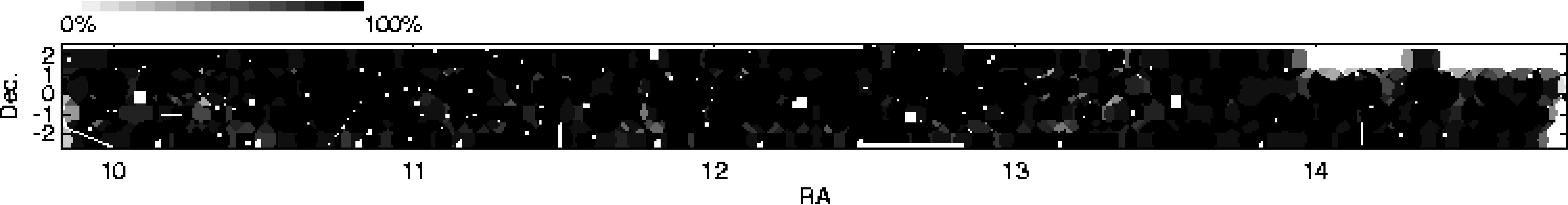
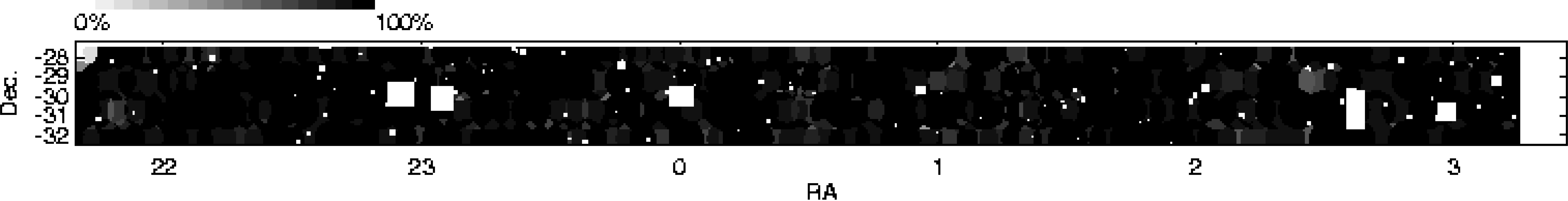
Figure 2: The coverage map for the 2QZ catalogue for the equatorial (top) and SGP (bottom) regions. The grey-scale indicates the percentage of 2QZ candidates observed over the two survey strips. Regions removed due to bright stars or plate features/defects can be seen, as can the unobserved fields at the 14^h end of the equatorial strip.

Spectroscopic observations of the input catalogue were made with the 2-degree Field (2dF) instrument at the Anglo-Australian Telescope (the 2QZ sample) and the 6-degree Field (6dF) instrument at the UKST (the 6QZ sample). The 2dF instrument is a multi-fibre spectrograph which can obtain simultaneous spectra of up to 400 objects at once over a $2^{\circ}$ diameter field of view, and is positioned at the prime focus of the Anglo-Australian Telescope. Fibres are robotically positioned within the field of view and are fed to two identical spectrographs (200 fibres each). Two field plates, and a tumbling system allow one field to be observed while a second is being configured, reducing down-time between fields to a minimum. The spectrographs each contain a Tektronix $1024\times 1024$ CCD with 24 $\mu$m pixels. Details of the 2dF instrument can be found in Lewis et al. (2002).

The 6dF instrument is a multi-fibre spectroscopic instrument on the UKST with the capability to simultaneously observe up to 150 sources over a $6^{\circ}$ diameter field of view. Fibres are positioned robotically onto a field plate, which is then installed at the focus of the UKST telescope. Fibres are fed to a bench mounted spectrograph containing an EEV $1032\times 1027$ CCD with 13 $\mu$m pixels. Further details can be found in Watson et al. (2000).

Based on the need to restrict the magnitude range of objects observed by 2dF (to reduce scattered light) and the observed surface density of candidates, objects in the input catalogue with $18.25<b_{\rm J}\leq 20.85$ were observed with 2dF and those with $16.0<b_{\rm J}\leq 18.25$ were observed with 6dF. Although the 6QZ sample is approximately 100 times smaller than the 2QZ, it is important in extending the coverage of the QSO OLF to almost a factor of 100 in luminosity based on a single homogeneous input catalogue.

Full details of the 2dF spectroscopic observations and subsequent catalogue were provided by Croom et al. (2001b) at the time of the initial 10k data release. We therefore only present a brief description in this paper, updating information where appropriate. 2dF spectroscopic observations began in January 1997 and were completed in April 2002. The spectral dispersion was 4.3Å pixel^-1, giving an instrumental resolution of 9Å. The spectra covered the wavelength range 3700–7900Å. Each 2dF field in the survey was observed for 3300 – 3600 secs, giving a median signal-to-noise ratio ($S/N$) of 5.0 per pixel in the $B$-band (4000–4900Å), see Fig. 1a. The data were taken in a wide variety of conditions. Under conditions of poor seeing ($>2\,$arcsec) or transparency, exposure times were increased to compensate for the lower signal rates. In the event that conditions prevented any field reaching its pre-determined completeness level, it was scheduled for re-observation (see below).

The 2QZ input catalogue was merged with that of the 2dF Galaxy Redshift Survey (2dFGRS; Colless et al. 2001) and a complex tiling algorithm was applied to the resultant joint catalogue in order to maximize the efficiency with which the two declinations strips could be covered with the minimum number of circular 2dF fields. The 2QZ survey area is an exact subset of the 2dFGRS area. Where possible, when conditions were unsuitable for the more exacting requirements of the 2QZ program (e.g. poor seeing, significant moonlight), observations of the 2dFGRS only fields were carried out.

6dF observations were performed over the period March 2001 – September 2002. The spectral range covered was 3900–7600Å using a low dispersion 250B grating which provided a dispersion of 286Å mm^-1 (3.6Å pixel^-1) and a spectral resolution of $\simeq 11.3$Å. Typical observation times were between 1.5 hours and 2 hours per field. An average of 50 6QZ objects were observed in each 6dF pointing. A median $S/N=16$ per pixel was obtained in the continuum of 6dF spectra (see Fig. 1b). This higher $S/N$ was set by our requirement to effectively identify the much larger numbers of contaminating stars in the 6QZ. A number of 6QZ targets where also observed in preliminary survey work carried out between September 1996 and December 1999 with the FLAIR spectrograph [Watson & Parker 1994] on the UKST prior to the commissioning of 6dF. These FLAIR spectra cover the range 3800–7300Å using the same 250B grating with $\simeq 11$Å resolution, but are generally lower $S/N$ than the 6dF data. All but a few (28) QSOs found with FLAIR have been re-observed with 6dF. FLAIR spectra are not available as part of the publically available database. Observations were obtained for candidates in both declination strips. However, the 6dF observations of the equatorial strip candidates are quite incomplete (less than 60 per cent of the candidates were observed), and so only the SGP strip is included in the final catalogue. In total, 25 overlapping 6dF pointings were used to cover the SGP strip.

2.3 Catalogue composition

Table 1: 2QZ/6QZ catalogue composition as a function of minimum sector completeness level (see text). The 70, 80 and 90 per cent columns give the properties of survey sub-samples which have those spectroscopic completenesses respectively. We list the number of objects in each of the different quality classes (Q1, Q2 and Q3). The final row gives the fraction (compared to the total number of observed sources) of IDs in each of the specified sub-samples and quality classes.

	2QZ												6QZ
	All			70 per cent			80 per cent			90 per cent			All
Class.	Q1	Q2	Q3	Q1	Q2	Q3	Q1	Q2	Q3	Q1	Q2	Q3	Q1	Q2	Q3
QSO	22655	683	–	20905	480	–	18068	312	–	11046	86	–	317	5	–
NELG	4484	74	–	4086	50	–	3458	31	–	2005	10	–	50	0	–
gal	79	16	–	73	11	–	59	6	–	34	1	–	1	0	–
star	10904	1388	–	9965	1007	–	8466	676	–	4996	168	–	1148	4	–
cont	102	52	–	84	41	–	68	28	–	24	12	–	3	1	–
??	–	–	4139	–	–	2749	–	–	1669	–	–	405	–	–	35
Total	38224	2213	4139	35113	1589	2749	30119	1053	1669	18105	277	405	1519	10	35
ID Frac	0.858	0.050	0.093	0.890	0.040	0.070	0.917	0.032	0.051	0.964	0.015	0.022	0.971	0.006	0.022

2.3.1 The 2QZ catalogue

2dF data were reduced at the telescope using the 2dF data-reduction pipeline 2DFDR [Bailey et al. 2003, Bailey & Glazebrook 1999] and information on the spectroscopic completeness achieved on each field was immediately fed back into the catalogue. 2dF fields which failed to achieve a pre-determined completeness level (either 70 per cent for the 2QZ or 90 per cent for the 2dFGRS) were scheduled for re-observation. In the end 556 out of 573 fields in the two 2QZ declination strips were observed. These included 10 fields that were kindly added to the equatorial strip when observations of 2QZ (and 2dFGRS) sources were made using spare fibres from spectroscopic follow up of the Millennium Galaxy Catalogue [Lemon, Driver & Cross 2001].

The coverage map for the 2dF survey is given in Fig. 2, showing the percentage of 2QZ targets that we obtained spectra for. We failed to obtain observations of a few 2dF fields in the most Northerly declination band of the equatorial strip at RAs greater than 14^h and a few fields at the very extreme edges/corners of both strips. In total, spectra were obtained for 44576 objects (93.3 per cent of the input catalogue) in the 2QZ, corresponding to an effective area of 673.4 deg². A small number of objects in the catalogue were observed not by 2dF, but by other instruments and/or telescopes. These are also included in our final catalogue. 111 equatorial sources with NVSS [Condon et al. 1998] radio detections and $b_{\rm J}<20$ were observed with the Low-Resolution Imaging Spectrograph on the Keck II Telescope [Brotherton et al. 1998]. Also, 69 targets were observed with either the Double-Beam Spectrograph (DBS) on the Siding Spring Observatory 2.3m Telescope, or the RGO Spectrograph on the AAT, as part of the follow up of close ($<20^{\prime\prime}$) QSO candidate pairs [Smith 1998]. DBS spectra of 20 objects in the 6QZ were also obtained.

Objects without spectra in the 2QZ either lie in the fields that were not observed by 2dF or in regions of high 2QZ/2dFGRS candidate surface density where the tiling algorithm was unable to configure a fibre observation efficiently given the minimum fibre-to-fibre spacing restriction ($\sim 30\,$arcsec). However, we note that 2QZ targets were given higher priority in the tiling algorithm than 2dFGRS targets, in order not to imprint the stronger angular clustering pattern of the galaxies onto the QSO distribution. Due to the significant amount of overlap between 2dF fields and the repeat observations of low completeness fields, 10528 objects (23.6 per cent) in the 2QZ have more than one spectroscopic observation.

Once reduced, 2QZ spectra were classified using the AUTOZ program (see Croom et al. 2001b) which uses a $\chi^{2}$-minimization technique to fit each spectrum to a number of QSO (BAL and non-BAL), galaxy and stellar templates and measure a redshift for all extra-galactic identifications. The QSO template was based on the composite spectrum of Francis et al. (1991). AUTOZ produces a single identification based on the best fit template in one of six categories based on the following spectral criteria:

QSO:	Broad ($>1000\,$km s-1) emission lines.
NELG:	Narrow ($<1000\,$km s-1) emission lines only.
gal:	Redshifted galaxy absorption features.
star:	Stellar absorption features at rest.
cont:	No emission or absorption features (High S/N).
??:	No emission or absorption features (Low S/N).

All AUTOZ identifications were independently checked visually by at least two members of the 2QZ team to correct any identifications that were clearly in error. Approximately 5 per cent of the AUTOZ identifications were changed in this fashion. As part of the classification process a quality flag was attached to each identification and redshift measurement as follows:

Quality 1:	High-quality identification or redshift.
Quality 2:	Poor-quality identification or redshift.
Quality 3:	No identification or redshift assignment.

The quality flag was determined independently for the identification and redshift of an object. For example, a quality 1 QSO identification could have a quality 1 or 2 redshift.

Table 1 gives the breakdown between the numbers identified in each class in the 2QZ. Fig. 3 shows the number-redshift relation, $n(z)$, for the QSOs and NELGs in the full 2QZ. The $n(z)$ histograms for both classes of objects are relatively smooth, indicating that there are no strong biases towards the selection of QSOs/NELGs over specific redshift intervals. The decline in QSO numbers at $z<0.4$ and $z>2.2$ are largely due to incompleteness in the colour and morphological selection process (see Section 3). We show the number counts, $n(b_{\rm J})$, for each identification class (omitting the small numbers of ’cont’ and ’gal’ identifications for clarity) in Fig 4. The surface densities are based on the observed counts divided by effective area of the full survey, with no further correction for incompleteness. At magnitudes fainter than $b_{\rm J}\sim 18.5$ mag the QSOs are the largest population, while at brighter magnitudes, galactic stars dominate.

The ’cont’ identification relates to potential BL Lac sources, however this class of object could be contaminated by other weak-lined objects (e.g. DC white dwarfs). To indicate the uncertainty inherent in this classification, in our final catalogue all ’cont’ IDs have quality 2. A more detailed investigation of possible BL Lacs in the survey has been carried out by Londish et al. (2002).

Figure 3: Number-redshift histograms for the 2QZ (upper panel) and 6QZ (lower panel) showing both QSOs (solid lines) and NELGS (dashed lines). The unshaded solid line includes all quality 1 and 2 QSOs, while the shaded histograms denote quality 2 QSO identifications only. Bin widths are $dz=0.025$ and $dz=0.25$ for the 2QZ and 6QZ respectively.

Figure 4: Number-magnitude counts for QSO (filled circle), NELG (filled triangle), Star (open triangle) and ?? (open circle) classifications in the 2QZ and 6QZ. Poisson error bars are shown.

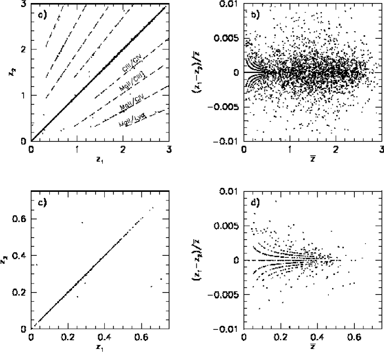
Figure 5: Redshift comparison for extra-galactic emission line objects in the 2QZ. a) $z_{1}$ vs. $z_{2}$ for QSOs. The dashed lines indicate the redshift differences caused by the confusion of specific QSO emission lines. b) Relative difference vs. mean $z$ for QSOs. c) $z_{1}$ vs. $z_{2}$ for NELGs. d) Relative difference vs. mean $z$ for NELGs. The quantization seen in b) and d) at low redshift is due to the redshifts being determined to a precision of 4 decimal places ($\sim 30$km s^-1). In all cases the determined redshift errors are considerably larger than this.

Of the 44576 objects with spectroscopic observations in the full 2QZ, 38224 received quality 1 IDs (85.8 per cent) 2213 quality 2 IDs (5.0 per cent) and 4139 quality 3 IDs (9.3 per cent).

We obtained a quantitative assessment of the quality flags from the objects with repeat observations. Based on the 5073 objects with quality 1 identifications and redshifts in two observations; 186 (3.7 per cent) had a different identification and different redshift. A further 38 (0.75 per cent) objects had a different identification, but the same redshift (to within $\Delta z=0.015$); arising as a result of a classification change from NELG to QSO or vice versa. 2697 objects with quality 1 IDs were classified as QSOs in both the observations, of these 2589 (96.0 per cent) had the same redshifts. Amongst the 615 objects classified as NELGs in both observations, 609 (99.0 per cent) were assigned the same redshift.

Of the 1026 objects with a quality 1 identification and redshift, but also a quality 2 identification, 334 (32.6 per cent) had a different identification and redshift. 21 (2.0 per cent) had a different identification but the same redshift. Of the 265 (14) objects that were classified as QSOs (NELGs) in both observations 185 (12) had the same redshift, or 70 (86) per cent of the respective populations.

Overall, we therefore conclude that the quality 1 identifications and redshifts are more than 95 per cent reliable, while the quality 2 identifications and redshifts are only reliable at the 70 per cent level.

We also obtained an estimate of the likely composition of the quality 3 object catalogue by looking at the 2735 quality 3 objects that were subsequently re-observed and given a quality 1 identification and redshift. Of these objects, 1611 (58.9 per cent) were classified as QSOs, 902 (33.0 per cent) as stars, 212 (7.8 per cent) as NELGs and 10 (0.4 per cent) as gals. This is close to the distribution of classifications in the full 2QZ (excluding ?? objects, see Table 1), with a slightly higher fraction (4 per cent) of stars and a lower fraction of NELGs amongst the unidentified objects. QSOs remain at an approximately constant 59 per cent of sources amongst both the identified and unidentified populations.

We can also increase the mean completeness of the 2QZ catalogue by limiting the sectors formed from the overlap of individual 2dF observations included in the catalogue to only those which meet a specified spectroscopic completeness threshold (see Section 3 below). Table 1 lists the composition of the catalogue based on a number of spectroscopic completeness thresholds set at 70 per cent, 80 per cent and 90 per cent (based on the percentage of quality 1 identifications in a given sector). By spectroscopic completeness we mean the fraction of spectroscopically observed sources for which we obtained a quality 1 identification. In most analysis that we have carried out with the 2QZ, we have used the 70 per cent sector spectroscopic completeness threshold to define the sample. Furthermore, we have only used objects with a quality 1 identification. These criteria were chosen to give the best compromise between maximizing the sample size (over 20000 QSOs) and minimizing spectroscopic incompleteness (11 per cent) in the 2QZ.

The repeat observations also provide a useful method to determine redshift accuracy. The RMS pairwise dispersion between redshift measurements for the 2589 QSOs with quality 1 redshifts and $\Delta z<0.015$ (excluding the objects with an incorrect redshift due to line mis-identification) is $\sigma(\Delta z)=0.0038$; giving a mean redshift error of $\sigma(z)=0.0027$ for an individual measurement. We note, however, that the dispersion increases as a function of redshift, from $\sigma(z,z<1)=0.0022$ to $\sigma(z,z>2)=0.0044$. A more z-independent estimate of the redshift error is given by the fractional error in the redshift $\sigma(z)/z=0.0027$, which is actually identical to the mean of $\sigma(z)$. A plot of the redshifts for the repeat observations with quality 1 identifications and redshifts is shown in Fig. 5. From this we can also see that the most common mis-identification was between the C IV $\lambda 1549$ and Mg II $\lambda 2798$ lines. For NELGs, the RMS dispersion in the redshifts $\sigma(\Delta z)=0.0005$, corresponding to a mean error in an individual redshift measurement error of $\sigma(z)=0.00035$.

2.3.2 The 6QZ catalogue

Table 2: Format for the 2QZ catalogue. The format entries are based on the standard FORTRAN format descriptors.

Field	Format	Description
Name	a20	IAU format object name
RA	i2 i2 f5.2	RA J2000 (hh mm ss.ss)
Dec	a1i2 i2 f4.1	Dec J2000 ($\pm$dd mm ss.s)
Catalogue number	i5	Internal catalogue object number
Catalogue name	a10	Internal catalogue object name
Sector	a25	Name of the sector this object inhabits
RA	i2 i2 f5.2	RA B1950 (hh mm ss.ss)
Dec	a1i2 i2 f4.1	Dec B1950 ($\pm$dd mm ss.s)
UKST field	i3	UKST survey field number
XAPM	f9.2	APM scan X position ($\sim 8$ $\mu$m pixels)
YAPM	f9.2	APM scan Y position ($\sim 8$ $\mu$m pixels)
RA	f11.8	RA B1950 (radians)
Dec	f11.8	Dec B1950 (radians)
$b_{\rm J}$	f6.3	$b_{\rm J}$ magnitude
$u-b_{\rm J}$	f7.3	$u-b_{\rm J}$ colour
$b_{\rm J}-r$	f7.3	$b_{\rm J}-r$ colour [including $r$ upper limits as: $(b_{\rm J}-r_{\rm lim})-10.0$]
$N_{obs}$	i1	Number of observations
Observation # 1
$z_{1}$	f6.4	Redshift
q1	i2	Identification quality $\times$ 10 + redshift quality
ID1	a10	Identification
date1	a8	Observation date
fld1	i4	2dF field number $\times 10$ + spectrograph number
fibre1	i3	2dF fibre number (in spectrograph)
$S/N_{1}$	f6.2	Signal-to-noise ratio in 4000–5000Å band
Observation # 2
$z_{2}$	f6.4	Redshift
q2	i2	Identification quality $\times$ 10 + redshift quality
ID2	a10	Identification
date2	a8	Observation date
fld2	i4	2dF field number $\times 10$ + spectrograph number
fibre2	i3	2dF fibre number (in spectrograph)
$S/N_{2}$	f6.2	Signal-to-noise ratio in 4000–4900Å band
$z_{\rm prev}$	f5.3	Previously known redshift (Véron-Cetty & Véron 2000)
radio	f6.1	1.4GHz Radio flux, mJy (NVSS)
x-ray	f7.4	X-ray flux, $\times 10^{-13}\,$erg s-1cm-2 (RASS)
dust	f7.5	$E(B-V)$ (Schlegel et al. 1998)
comment1	a20	Specific comments on observation 1
comment2	a20	Specific comments on observation 2

An identical procedure was followed to reduce the 6dF data and carry out the spectroscopic identification of the 6QZ. In total, 6dF spectra were obtained for 1564 of the 1657 colour-selected candidates (94.4 per cent) in the SGP strip, giving an effective area of 333.0 deg².

The composition of the 6QZ catalogue is given in Table 1. The 6QZ contains a much higher fraction of galactic stars (73.7 per cent of observed sources) and a correspondingly lower fraction of QSOs (20.6 per cent) given its brighter magnitude limit. The number-redshift relation for the QSOs and NELGs in the 6QZ is shown in Fig. 3. The $n(b_{\rm J})$ relation is shown in Fig. 4. We note that the QSO $n(b_{\rm J})$ relation fits smoothly onto that obtained for the 2QZ at $b_{\rm J}=18.25$, while the stellar $n(b_{\rm J})$ relation obtained for the 6QZ lies approximately a factor 2 lower than expected from an extrapolation of the 2QZ stellar counts. This reflects the more restrictive colour cut, $(u-b_{\rm J})\leq-0.50$, used to select the 6QZ candidate list. At this cut, the vast majority of the stars identified have been scattered into this sample by photometric errors. This explains the increase in the stellar surface density at the very brightest magnitudes ($b_{\rm J}<17\,$mag), where the photometric errors on the photographic magnitudes increase.

The 6QZ also has a much higher spectroscopic completeness level (over 97 per cent for quality 1 identifications) than the 2QZ and so we choose to make no further cuts on the basis of sector completeness as we did for the 2QZ. The higher completeness levels are directly attributable to the much higher mean S/N obtained for the 6dF observations.

Repeat observations were obtained for 475 objects in the 6QZ. Based on a similar comparison of the quality 1 identifications and redshifts to that carried out for the 2QZ sample, we conclude that the quality 1 identifications in the 6QZ are 99 per cent accurate (only 2 out of 254 repeat quality 1 identifications changed between observations) and the quality 1 redshifts are over 96 per cent accurate (only 6 out of 177 QSO redshift measurements differed by more than $\Delta z=0.015$, and of these, only one QSO had $\Delta z>0.03$).

We obtain a redshift error of $\sigma(z)=0.0026$ for the 6QZ QSOs, identical to that obtained for the 2QZ, based on a comparison of the redshifts obtained for the 171 QSOs in the 6QZ with repeated quality 1 observations with $\Delta z<0.015$.

2.4 Data Products

The 2QZ and 6QZ catalogues are available as ASCII files from the 2QZ WWW site, http://www.2dfquasar.org, and on a CD-ROM release. The catalogue format is identical for both surveys and is given in Table 2. Note that the catalogue format has been extended to include more information since the preliminary data release [Croom et al. 2001b]. The first part of a catalogue entry contains details from the input catalogue, such as position and magnitude. We note that the object names may in some cases not correspond exactly to the source position in $\alpha$ and $\delta$ as we have improved the astrometry of the catalogue [Smith et al. 2003] since the object names were defined. The names have not been changed subsequently, to avoid confusion with previously published lists. We now include internal catalogue names and numbers, although objects should generally be referenced by their main IAU format name. A new entry is included for the name of the sector inhabited by the object. A sector is defined as the intersection of overlapping 2dF fields (see Section 3). The format of these is e.g. S_200_201_247, where the S denotes the SGP strip and the numbers indicate that the sector is formed by the overlap of fields 200, 201 and 247. There are no sectors defined for the 6QZ. Coordinates are also supplied in the B1950 system, as the survey was constructed in this system and the production of completeness masks etc. is more straight forward in this system. We also note that sources which had only upper limits (i.e. non-detections) on the $r$ plates are also included in the catalogue and have a listed $b_{\rm J}-r$ colour. In this case the colour term is $(b_{\rm J}-r_{\rm lim})-10$, the $-10$ being used to differentiate upper limits from normal colours (objects with real $r$-band detections have colours in the range $-1.4<b_{\rm J}-r<3.4$, while upper limits have $b_{\rm J}-r<-9.8$).

The input catalogue information is followed by details of observations and identifications. As discussed above, in a number of cases we have two or more 2dF observations of the same source. The first and second observations (arranged in quality order) are listed in the main catalogue. These are useful to assess the quality of the final catalogue. The identification and redshift that we adopt is that from the observation with the numerically lowest quality value (where the quality value is identification quality$\times 10$ + redshift quality), and if there are equal quality values, the highest S/N. In all cases the final adopted ID is listed as observation #1, with the lower quality observation being listed as observation #2. We also list the 2dF field number (fld₁ and fld₂) for each observation. These correspond to the actual 2dF field number $\times 10$ + the spectrograph number (1 or 2 for 2dF, 6 for 6dF). Sources with spectra from the Keck observations of 2QZ radio sources all have field number 8881. Sources from the followup of close pairs have field number 7771. Sources from the 6QZ with DBS observations have field number 6666. We also include cross-matches to selected other databases. Where a 2QZ/6QZ source matches the position (to within $6^{\prime\prime}$) of a previously known QSO/AGN in the catalogue of Véron-Cetty & Véron (2000) we include the previously known redshift. We also include radio fluxes at 1.4GHz from the NRAO VLA Sky Survey (NVSS; Condon et al. 1998) and X-ray fluxes from the ROSAT All Sky Survey (RASS; Voges et al. 1999; Voges et al. 2000), converting from RASS counts per second to flux (in erg s^-1cm^-2) by multiplying by $1.2\times 10^{-11}$. The matching radii used were $15^{\prime\prime}$ and $30^{\prime\prime}$ for NVSS and RASS respectively. An estimate of the galactic reddening $E(B-V)$ to each source is taken from the work of Schlegel, Finkbeiner & Davis (1998). In order to convert from $E(B-V)$ to extinction values multiply by 5.434, 4.035 and 2.673 for $A_{\rm u}$, $A_{\rm b_{\rm J}}$ and $A_{\rm r}$ respectively. Lastly we supply any comments made on the particular observation which might flag the object or spectrum as unusual.

For the catalogue we have not attempted to sub-divide the NELG class into LINERs, Seyferts, starbursts, etc. Given the finite spectral window of the 2QZ and 6QZ observations and the large redshift range observed for NELGs ($0<z<0.6$), in many case key diagnostic lines required for further spectral classification are missing from the spectra. The spectral coverage provided by 2dF and 6dF limits our ability to detect broad Mg II emission until $z>0.35$. In some QSOs with $0.35<z<0.5$, broad Mg II is clearly detected with no corresponding broad H$\beta$ seen. Thus at lower redshifts, $0.15<z<0.35$, some objects classified as NELGs on the basis of a narrow H$\beta$ line may exhibit broad Mg II below the blue limit of the 2dF spectral window. For QSOs with $z>1.6$, AUTOZ fits both ‘normal’ and BAL QSO templates. Objects identified as BALs are indicated by ‘QSO(BAL)’ in the identification column. However, due to the varied nature of BAL QSOs, this will not be a comprehensive list of BALs. A more detailed search for BALs has not yet been applied.

Within the objects we classify as stars, in the main we only give classifications for white dwarfs (WDs). We have not attempted to provide spectral classification of main sequence stars. The $\sim 2000$ WDs are mostly DAs with strong broad hydrogen Balmer absorption lines. At low S/N these can be confused with A stars. Only detailed fitting of the temperature and gravity of these stars can easily resolve this issue, and this is beyond the scope of the present paper. As well as DAs we also find a number of DB and DO WDs which are dominated by neutral and singly ionized helium respectively. A small number of DZs are also found, with broad Ca II H and K $\lambda\lambda 3969,3933$ absorption. The only other stellar types we classify are emission line stars with strong hydrogen Balmer emission which we classify as CV (cataclysmic variable) and WD + M dwarf binary systems which are denoted as DAM, DBM etc. We note that our code has been designed primarily to simply identify an object as a star (and therefore not a QSO), and that a more detailed analysis would no doubt provide more accurate classifications. Some analysis of the Galactic stars in the 2QZ has already taken place [Vennes et al. 2002, Marsh et al. 2002]. The above classifications are denoted within the catalogue in parentheses after the main star identification [e.g. star(DB), star(CV)].

FITS format spectra for all objects, including repeat observations and spectra from which no identification was possible, are provided as a primary data product of the 2QZ and 6QZ surveys at http://www.2dfquasar.org/ and on the survey CD-ROM. Note that many of the repeat spectra are of low quality, as the fields were repeated if they had low completeness. A small fraction of spectra have bad ’fringing’ caused by a damaged fibre. This shows up as a strong oscillation as a function of wavelength, rendering the underlying spectrum unusable. In a few cases 2DFDR failed to cope adequately with the sky subtraction process at either end of the CCD data-frame and so a number of spectra have poorly subtracted night sky emission (and in some cases moonlight) which has also affected our ability to identify an object in some cases. The spectral database does not include spectra from FLAIR observations. It also does not include spectra from the small number of 2QZ identifications not based on 2dF spectra (see Section 2.3.1).

On the WWW site, we also provide 1-arcmin square SuperCOSMOS-scanned images [Hambly et al. 2001] of the $J$ photographic plates around each object in the 2QZ and 6QZ catalogue. Due to space restrictions, these images are not available on the CD-ROM. The input catalogue is also available from this site [Smith et al. 2003]. The input catalogue, spectroscopic catalogue, FITS spectra and photographic images define the primary data products of the 2QZ and 6QZ surveys. To aid in the interrogation and analysis of the catalogue, we also provide a web search tool, scripts/code used to generate the survey mask for an arbitrary minimum sector completeness and the $\alpha,\delta$ of the survey boundaries/holes drilled around bright stars in the input catalogue. We also provide quantitative estimates of catalogue completeness for QSOs, where appropriate, as a function of magnitude, redshift and position in 2QZ and 6QZ catalogues. The empirical methods used to define these completeness estimates, arising from a variety of sources are discussed in turn in the following section.

3 Survey completeness

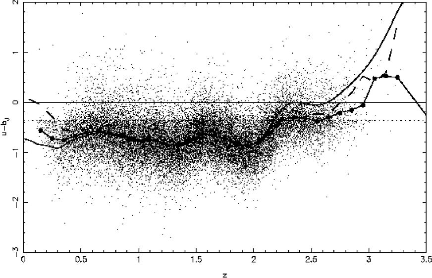
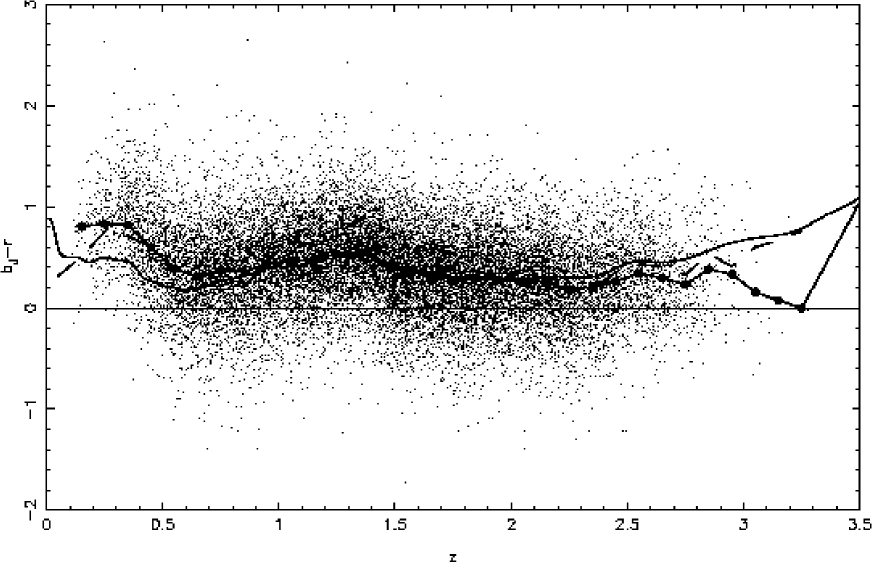
Figure 6: The colour redshift relations for the 2QZ/6QZ sample. Top: $u-b_{\rm J}$ vs. $z$ for all quality 1 QSOs. The dotted line indicates the $u-b_{\rm J}=-0.36$ selection limit. Bottom: $b_{\rm J}-r$ vs. $z$ for quality 1 QSOs. The connected filled circles show the mean colours in $\Delta z=0.1$ bins. The solid line describes the colours derived from the SDSS composite spectrum, zero-pointed to the 2QZ at $z=1-2$. The dashed line describes the mean colours of the Hawkins (priv. comm.) variability selected sample.

We now come to discuss the survey completeness, and sources of incompleteness. We define four separate types of completeness that can be used to describe the 2QZ and 6QZ surveys. These are:

• Morphological completeness, $f_{\rm m}(b_{\rm J},z)$. This describes our effectiveness at differentiating between point sources and extended sources on UKST plates, and also the possible effect of the QSO host galaxies on morphology at low redshift.

• Photometric completeness, $f_{\rm p}(b_{\rm J},z)$. This attempts to take into account any QSOs which may have fallen outside of our colour selection limits.

• Coverage completeness (or coverage), $f_{\rm c}(\theta)$. We define the coverage as the fraction of 2QZ catalogue sources which have spectroscopic observations.

• Spectroscopic completeness, $f_{\rm s}(b_{\rm J},z,\theta)$. This is the fraction of 2QZ catalogue objects which have the specified quality of spectrum (in our case we consider quality 1 identifications).

We indicate against each type of completeness above whether it is considered to be a function of angular position $\theta$, magnitude $b_{\rm J}$, or redshift $z$. To provide a general description of the angular positional dependence of completeness we determine completeness values within each of the regions which are described by sets of our overlapping $2^{\circ}$ diameter fields. Within each of these regions, which we call sectors, we may define a coverage and spectroscopic completeness value. For ease of use these completeness maps are then pixelized on a scale of 1 arcminute. Below we describe each of these different completeness measurements and the corrections which can be applied to account for them. For some analyses it is appropriate to define such completeness on an object-by-object basis.

3.1 Morphological completeness

Morphological completeness falls into two categories. The first concerns objects which are truly point-sources, but which have been mis-classified by the APM analysis software. The second concerns QSOs which have significant host galaxy contributions, which make their images non-stellar. This is an issue at low redshift ($z<0.4$).

The first of these two classes of morphological completeness is by far the easiest to quantify. A small fraction of stellar objects are classified as merged images or galaxies by the APM on the basis of random errors or overlapping images on the photographic plate. The fraction of sources classified as non-stellar ($f_{\rm ns}$) and lost in this fashion has been determined by direct comparison with the SDSS Early Data Release [Stoughton et al. 2002] imaging data in the equatorial region where the surveys overlap [Smith et al. 2003] and is well described by

$$f_{\rm ns}=0.064+0.0052(b_{\rm J}-16).$$ (1)

$f_{\rm ns}$ thus varies between 0.064 and 0.089 over the full magnitude range covered by the 2QZ and 6QZ surveys. We see no systematic variations in $f_{\rm ns}$ as a function stellar density, which varies along the survey strip.

Since QSO candidates were selected on the basis of their stellar appearance on photographic plates, low redshift QSOs with detectable host galaxies on the plate will also be preferentially de-selected from the final input catalogue. The visibility of QSO host galaxies on photographic plates is extremely difficult to model; given the large variation in host galaxy properties and the large scatter in the relation between host and nuclear luminosities (Schade, Boyle & Letawsky 2000). However, the 2QZ should be relatively free of morphological bias against ’extended’ QSOs for $z>0.4$, at which even the largest host galaxies ($r_{\rm e}\simeq 10\,$kpc), will have angular size of less than 2 arcsec, and therefore appear unresolved on the photographic plates with stellar image size typically 2–3 arcsec. This is further substantiated by Hewett, Foltz & Chaffee (1995) who find an excess of extended sources in the Large Bright Quasar Survey (LBQS), only at $z<0.4$. Also, Meyer et al. (2001) find that 4 out of 71 QSOs found in the Fornax Cluster Spectroscopic Survey (FCSS) are extended from APM scans, but that these are generally mis-classifications due to nearby bright stars and galaxies. It should be noted however, that the LBQS and FCSS have brighter flux limits, $b_{\rm J}\simeq 18.8$ and $b_{\rm J}\simeq 19.7$ respectively, than the 2QZ. With brighter nuclei, the effect of the host galaxies in determining the observed morphology will be reduced.

We therefore choose not to derive any completeness correction for the morphological effect of host galaxies. For many applications where the QSO space density is normalized to a local mean (e.g. clustering) any $z$-dependent bias (morphological or otherwise) can be corrected as part of normalization to the observed $n(z)$ relation as long as that bias is a smooth, slowly varying function of redshift.

3.2 Photometric completeness

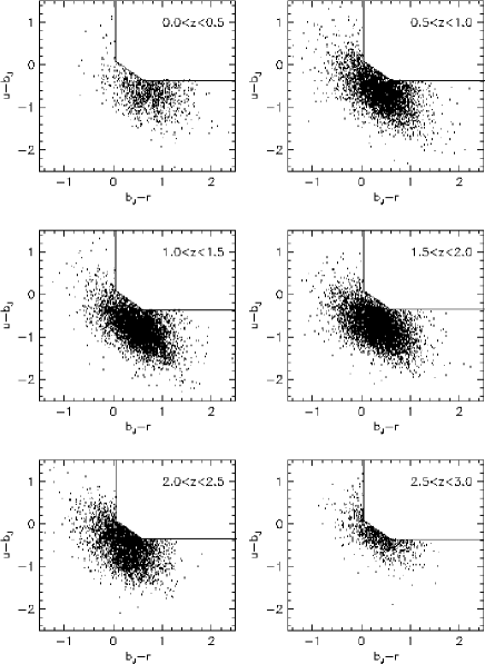
Figure 7: Colour-colour plots for 2QZ/6QZ QSOs in redshift bins of $\Delta z=0.5$. The solid lines indicate our colour selection limits. At low redshift ($0.0<z<0.5$) the QSO colours are redder in $b_{\rm J}-r$, therefore the $u-b_{\rm J}$ cut has greater impact on selection. At high redshift ($z>2$) the QSO colours become increasingly red, until the predicted centre of the locus is within the region excluded by our colour selection limits.

Photometric incompleteness is caused by errors in the photographic magnitudes ($\sim$0.1 mag in each band) and variability (due to the non-contemporaneous nature of the $ub_{\rm J}r$ plates on each field) which cause QSOs to exhibit $u-b_{\rm J}/b_{\rm J}-r$ colours outside our selection criteria. It could also be the case that we are missing some fraction of the QSO population that are intrinsically red, however the fraction of red QSOs in a $b_{\rm J}$ flux limited sample is likely to be small [Meyer et al. 2001]. Hewett, Foltz & Chaffee (2001) also find that the fraction of objects missed from the blue selected LBQS is only $13\pm 4$ per cent, using matches to the FIRST radio survey [Becker et al. 1995]. Given the uncertain nature of any red QSO population we chose to base our photometric completeness estimates on the likelihood of detecting typical blue QSOs. In order to fully quantify the incompleteness due to our colour selection we have adopted a semi-empirical approach. This allows us to make use of the measured properties of the 2QZ QSOs as well as theoretical estimates of QSO colours. We derive the mean QSO colours in $u-b_{\rm J}$ and $b_{\rm J}-r$ as a function of $z$ and $b_{\rm J}$ and use this in combination with the measured dispersion of 2QZ QSOs about the mean to model the colour distributions. Applying our selection criteria to these model QSO colours allows us to determine the fraction of QSOs that would have been selected.

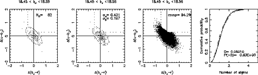
Figure 8: Fitting of the $u-b_{\rm J}$ vs. $b_{\rm J}-r$ colour distribution for two example magnitude intervals. Top: $18.45<b_{\rm J}<18.55$, Bottom: $20.45<b_{\rm J}<20.55$. From left to right the plots are: a) colour distributions relative to the mean for QSOs with $1\sigma$ and $2\sigma$ fitted contours. $N_{\rm Q}$ is the number of QSOs in the plot. b) Grey-scale of the same distribution, showing the fitted $\sigma$ values. c) A random realization of the fitted model with 10000 points and an estimated completeness value. d) A K-S test between the radial distributions of the QSOs and random points.

Our first step is to derive the mean colour-redshift relations for the 2QZ. The $u-b_{\rm J}$ and $b_{\rm J}-r$ colours of 2QZ/6QZ QSOs are shown in Fig. 6 as a function of redshift (small points), also shown are the mean colours in $\Delta z=0.1$ intervals (connected filled circles). The $u-b_{\rm J}$ vs. $z$ colours show slow variations due to various emission lines moving in and out of the bands, and an up-turn at $z=2$ where Lyman-$\alpha$ moves from the $u$-band to the $b_{\rm J}$-band, and the $u$-band becomes increasingly affected by Lyman-$\alpha$ forest absorption. At low redshift ($z<0.5$) we also see evidence of a move red-wards in the QSO $u-b_{\rm J}$ and $b_{\rm J}-r$ colours. This is most noticeable in the mean $b_{\rm J}-r$, as sources with redder $u-b_{\rm J}$ colours tend not to be selected. Indeed, while at most redshifts there is little evidence of a sharp drop in QSO numbers redder than the $u-b_{\rm J}$ cut (dotted line), this is not the case at $z<0.5$ where most QSOs selected are bluer than the $u-b_{\rm J}$ cut. This effect is most clearly seen in Fig. 7 which displays the $u-b_{\rm J}$ vs. $b_{\rm J}-r$ colours of 2QZ/6QZ QSOs in redshift bins of width $\Delta z=0.5$. At $z<0.5$ the QSO locus is more affected by the $u-b_{\rm J}$ colour cut, due to the redness of the $b_{\rm J}-r$ colours. This reddening at low redshift is probably due to the increasing amount of contamination from the host galaxies of the QSOs, confirmed by the appearance of host galaxy features (Ca II H & K) in the spectra of low redshift QSOs in the 2QZ [Croom et al. 2002]. At high redshift ($z\sim 2.5$ and greater) mean QSO colours lay within the region excluded from our analysis by our colour selection limits, and QSOs that are detected are found close to the colour selection limits.

We then compared the 2QZ colours to those derived from the SDSS composite QSO spectrum [Vanden Berk et al. 2001], taking the SDSS composite and convolving it with the $u$, $b_{\rm J}$ and $r$ band passes (using those specified by Warren et al. (1991) and references therein), and then zero-pointing the magnitudes to the mean 2QZ colours at $z=1-2$. The required shifts are an addition of 0.16 and $-0.08$ mag to the model $u-b_{\rm J}$ and $b_{\rm J}-r$ colours respectively. We have examined the uniformity of the 2QZ colours by comparing the median QSO colours in each UKST field. The rms scatter found is 0.03 mags, fully consistent with the minimum errors typically achievable with photographic plates. Detailed tests of the procedure used to generate the synthetic colours found no significant errors. The exact source of the above zero-point offsets in unclear, but as the 2QZ photometry is internally consistent and our completeness estimates are largely empirical these offsets should not cause any systematic errors in our analysis of the survey completeness.

We see that the $u-b_{\rm J}$ and $b_{\rm J}-r$ SDSS colours (solid lines in Fig. 6) are very close to those of the 2QZ over the redshift range $z=0.5-2.0$. At higher redshift, the SDSS colours are redder than those from the 2QZ, as Lyman-$\alpha$ absorption progressively reddens the QSO colours. This demonstrates that the 2QZ completeness starts to decline past $z=2$ as we preferentially select only the bluest QSOs at these redshifts. We also note that the SDSS colours are bluer in both $u-b_{\rm J}$ and $b_{\rm J}-r$ than the 2QZ at $z<0.4$. We attribute this to the decreased effect of the host galaxy in the higher luminosity (typically 1 mag) QSOs sampled by the SDSS survey; based on the flat relation between nuclear and host luminosities for QSOs ($L_{\rm QSO}\propto L_{\rm gal}^{0.2-0.4}$) [Schade et al. 2000, Croom et al. 2002]. In the SDSS composite this could also be due to contamination at low redshift by narrow emission line galaxies [Vanden Berk et al. 2001], as well as the fact that because there are many more QSOs found at high redshift, the higher redshift QSOs (with less contribution from the host galaxy) will dominate the construction of the composite spectrum.

We also compare the 2QZ/6QZ QSO colours to a sample of QSOs which have been selected on the basis of their variability (Hawkins & Veron 1995; Hawkins private communication). We derive the mean $u-b_{\rm J}$ and $b_{\rm J}-r$ colours for Hawkins QSOs with $b_{\rm J}<21$ as a function of redshift and plot them in Fig. 6 (dashed lines). They are zero-pointed to the mean 2QZ/6QZ colours at $z=0.7-2.0$. These shifts are slightly larger than those derived above for the model colours based on the SDSS QSO composite and are an addition of $-0.27$ and $-0.16$ mag to the derived $u-b_{\rm J}$ and $b_{\rm J}-r$ colours of the Hawkins sources), and may be due to a zero-point offset in the Hawkins photometry. Once this zero-point shift has been accounted for the mean Hawkins colours follow closely the mean 2QZ/6QZ colours at $0.5<z<2.3$. At higher redshift they become redder than the 2QZ/6QZ, as do the SDSS colours. At lower redshift the Hawkins $b_{\rm J}-r$ colours are close to the 2QZ/6QZ colours at $z>0.2$, but the Hawkins $u-b_{\rm J}$ are significantly redder than those of the 2QZ/6QZ. As the Hawkins variability selected QSOs are not selected on the basis of colour, they should, to first order, be independent of colour, and thus follow more closely the true colour distribution of the QSO population. We do note, however, that certain issues can affect variability selection, such as host galaxy contamination, the correlation of variability with luminosity and redshift (e.g. Trèvese & Vagnetti 2002), and these may introduce some colour dependence to any variability selected sample.

The above considerations suggest that we use the following to define our mean QSO colour-redshift relations: i) the mean Hawkins colours for $u-b_{\rm J}$ at $z<0.5$; ii) the mean 2QZ/6QZ colours for $u-b_{\rm J}$ at $0.5<z<2.0$ and $b_{\rm J}-r$ at $0.0<z<2.0$; iii) the SDSS composite colours at $z>2.0$ for $u-b_{\rm J}$ and $b_{\rm J}-r$. We note that in each case the SDSS composite and Hawkins colours have had the above zero-point shifts applied.

A final point to consider is whether there is any magnitude dependence of the mean colours. In particular, if the reddening of the $b_{\rm J}-r$ colours at low $z$ is due to increasing host galaxy contamination, this effect might be most noticeable in intrinsically faint QSOs. We find this to be the case for 2QZ/6QZ $b_{\rm J}-r$ colours. The variation in colour can be described by

$$\Delta(b_{\rm J}-r)=-9.17+0.479b_{\rm J}+13.1z-0.685b_{\rm J}z$$ (2)

at $z<0.70$. At higher redshift no significant effect is seen. We see no similar reddening of the $u-b_{\rm J}$ colours towards fainter magnitudes for low redshift QSOs in the 2QZ/6QZ, although some weak dependence would be expected if it is the host galaxy which is producing the variation in $b_{\rm J}-r$ colours. We have tested the expected $\Delta(u-b_{\rm J})$ for a given $\Delta(b_{\rm J}-r)$ by combining the SDSS QSO composite spectrum and model galaxy spectra. For a range of galaxy SEDs (e.g. single instantaneous bursts of star formation of age between 3 and 10 Gyr) the typical $\Delta(u-b_{\rm J})$ is between $\sim 0.2$ and 0.5 times $\Delta(b_{\rm J}-r)$ above $z\sim 0.2$. As the exact nature of this correction is difficult to model due to uncertainties in the galaxy SED and the fractional contribution of the host, and we do not see any evidence of a magnitude dependence of the mean $u-b_{\rm J}$ colours, we have decided not to make any correction to the mean $u-b_{\rm J}$ as a function of QSO magnitude. We therefore correct our mean colour-redshift in $b_{\rm J}-r$ only by an amount defined from Eq. 2, although we limit the $b_{\rm J}-r$ colours to be no bluer than those from the SDSS composite.

Figure 9: The semi-major axis (filled circles) and semi-minor axis (open circles) dispersions for the 2D Gaussian distribution fitted to the colour-colour distributions as a function of magnitude. The solid lines denote the best fit lines used to derive the model QSO colour distributions. At bright magnitudes the dispersions are forced to be no less than the mean dispersion found at $b_{\rm J}=17-18$.

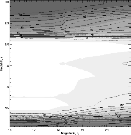
Figure 10: Photometric completeness contours in the ($b_{\rm J},z$) plane for the 2QZ. The contours are plotted at 5 per cent intervals: dotted lines denote 5, 15, 25,…95 per cent completeness; solid lines correspond to 10, 20, 30…90 per cent.

Once the mean colour-redshift relations are defined, we then determine the dispersion about the mean. In doing this we assumed that the dispersion was a function of magnitude only, a reasonable assumption given that photometric errors and variability dominate the scatter. Any redshift dependence of variability was considered to be a second order effect. The dispersion about the mean $u-b_{\rm J}$ and $b_{\rm J}-r$ colours was fit by a 2D Gaussian distribution in $\Delta b_{\rm J}=0.1$ intervals between $z=1$ and 2. This redshift range was chosen as the regime where completeness was highest, so as to give the most accurate description of the QSO colour distribution. Two examples of these fits are shown in Fig. 8. Regions outside of our colour selection limits were not included in the fitting procedure. We first attempted to fit the colour distribution with four parameters: peak height, semi-major axis ($\sigma_{\rm a}$), semi-minor axis ($\sigma_{\rm b}$) and position angle. However investigation showed that in all cases the position angle was close to 45^∘. The fitting process was then repeated fixing the position angle to be 45^∘. Random distributions following the fitted Gaussian were produced to confirm that the 2D Gaussian was a reasonable fit to the data via a radial Kolmogorov-Smirnov (K-S) test. Only two $\Delta b_{\rm J}=0.1$ intervals showed a significant difference between the data and the model. In general we note that the model does generate marginally less extreme outliers in the colour distributions, however this does not significantly affect the determined completeness values. The measured widths of the 2D Gaussian model were fitted by a straight line in the range $17<b_{\rm J}<20.85$, and these fits used to determine the dispersion in our final Monte-Carlo simulations that estimate QSO completeness. At $b_{\rm J}<17$ there are insufficient QSOs to make an adequate fit to their distribution, so the dispersions are fixed to be the mean of the dispersion in the $b_{\rm J}=17-18$ range (see Fig. 9).

Finally we make Monte-Carlo simulations of the QSO colour distributions in $\Delta b_{\rm J}=0.1$ and $\Delta z=0.1$ bins using 100000 QSOs in each interval. The fraction of simulated QSOs which fall outside our colour selection limits then define our incompleteness. The final photometric completeness contours are shown in Fig. 10. The photometric completeness is largely independent of magnitude and is at least 70 per cent or greater over the redshift range $0.4<z<2.2$. At higher redshifts the completeness rapidly drops, falling to below 50 per cent at $z>2.3$. The bluer $u-b_{\rm J}$ limit imposed on the 6QZ ($u-b_{\rm J}<-0.5$ rather than $u-b_{\rm J}<-0.36$) causes a weak step in the completeness contours which can be seen at $b_{\rm J}=18.25$.

3.3 Coverage completeness

Figure 11: The ratio of close pairs found in the 2QZ input catalogue, $NN_{\rm c}$ to those observed with 2dF $NN_{\rm obs}$. At scales less that $\sim 1-2$ arcmin there is a decrease in the number of pairs due to the positioning constrains of the 2dF fibre positioner. The constant offset below 1 at larger angular scales is cause by the lower mean density of observed objects compared to the full catalogue (i.e. not all objects could be observed).

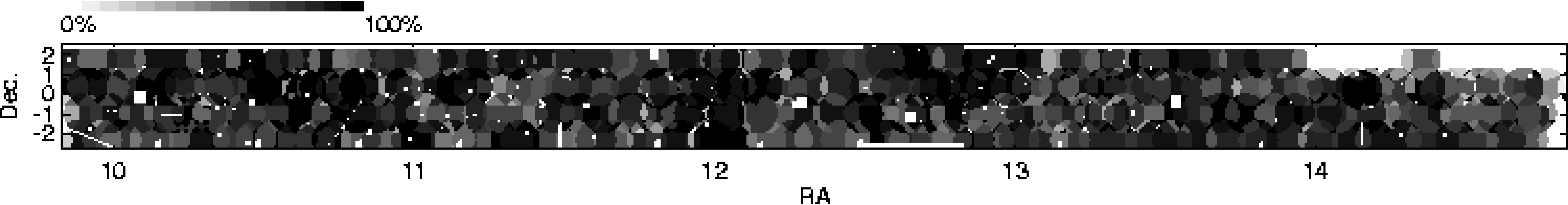
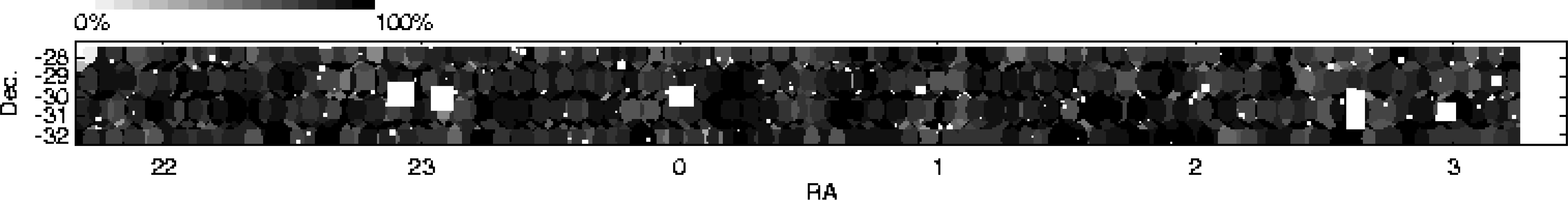
Figure 12: The completeness map of the 2QZ catalogue for the equatorial (top) and SGP (bottom) regions. The grey-scale indicates the percentage of 2QZ candidates observed and positively identified (quality 1) over the two survey strips. This is equivalent to $f_{\rm c}(\theta)f_{\rm s}(\theta)$.

Of all four types of completeness, at a sector level the coverage completeness (or coverage) is the simplest to derive, being only a function of angular position. We define the coverage as being the ratio of observed to unobserved sources in each of the sectors defined by overlapping 2QZ fields, we denote this by $f_{\rm c}(\theta)$. The coverage maps (pixelized on 1 arcminute scales) of the two 2QZ strips are shown in Fig. 2. These maps also account for holes in the survey regions which are due to bright stars or photographic plate defects/features. The incompleteness in coverage arises from the difficulty of configuring all targets onto 2dF fibres using the adaptive tiling scheme [Colless et al. 2001]. This is caused by variations in target density, a small (typically $\sim 1$ per cent) number of broken or unusable 2dF fibres, and constraints due to the minimum fibre spacing ($\sim 30$ arcsec). These issues are in large part alleviated by the large overlaps between 2dF fields, however it was still not possible to observe 100 per cent of the QSO candidates in the 2QZ. The remaining decline in the number of close pairs is demonstrated in Fig. 11 which shows the ratio of close pairs from observed ($NN_{\rm obs}$) to those in the input catalogue ($NN_{\rm c}$). This shows a decline in close pairs at angular scales less than $\sim 1-2$ arcmin. This has no significant effect on the clustering analysis of QSOs (e.g. see Croom et al. 2001a). The number of close pairs contained within the input catalogue is also limited by the resolution available on the APM scans of our UKST plate material. This reduces the number of close pairs on angular scales less than $\sim 8$ arcsec [Smith et al. 2003].

3.4 Spectroscopic completeness

3.4.1 Position dependent spectroscopic completeness, $f_{\rm s}(\theta)$

Spectroscopic completeness is perhaps the most complex of all completenesses to describe. In our discussion below we focus on the spectroscopic completeness of the QSOs in our survey, as they are the primary targets of our observations. In general different classes of object will have different spectroscopic completeness functions, e.g. NELGs are more easily identified in low $S/N$ spectra than stars. Our assessment of QSO spectroscopic incompleteness assumes that there are equal fractions of QSOs among both the identified and unidentified spectra (see Section 2.3.1). Alternative methods may be required to assess the completeness of different object classes.

The distribution of combined coverage and spectroscopic incompleteness, $f_{\rm c}(\theta)f_{\rm s}(\theta)$, across the two 2QZ strips based on quality 1 IDs alone is shown in Fig. 12 (c.f. Fig. 2 which shows the coverage incompleteness only). However, this only describes the mean spectroscopic completeness in each sector (i.e. as a function of angular position). This is straightforward to calculate on a sector-by-sector basis, based on the ratio $N_{1}/N_{\rm obs}$, where $N_{1}$ is the number of quality 1 IDs in a sector and $N_{\rm obs}$ is the number of targets observed in a sector. By contrast, $f_{\rm c}$ is determined by the ratio $N_{\rm obs}/N_{\rm c}$, where $N_{\rm c}$ is the total number of 2QZ sources within the sector. However, while coverage is only dependent on angular position, spectroscopic completeness will in general also be dependent on $b_{\rm J}$ and $z$. For many analysis (e.g. the luminosity function, see below), we only require global magnitude and redshift dependent corrections. These will vary with the minimum sector completeness level applied to produce any ‘complete’ spectroscopic catalogue (see Section 2.1). For example the inclusion of more low mean completeness sectors will produce a spectroscopic completeness function with a more marked dependence on $b_{\rm J}$.

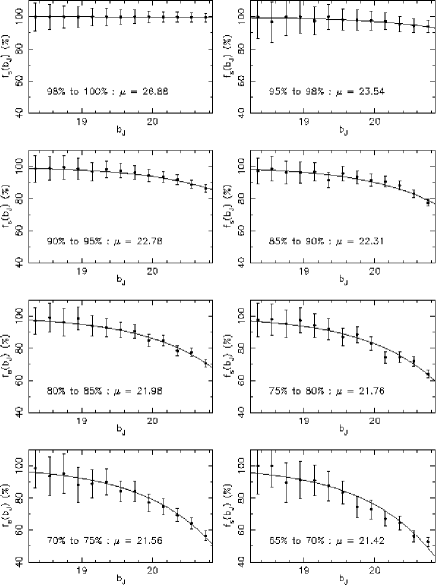
Figure 13: Spectroscopic completeness as a function of $b_{\rm J}$ magnitude, $f_{\rm s}(b_{\rm J})$, for sectors with different mean completeness values, $f_{\rm s}(\theta)$ (filled circles). These are plotted for mean sector completeness intervals 0.98–1.00, 0.95–0.98, 0.90–0.95, 0.85–0.90, 0.80–0.85, 0.75–0.80, 0.70-0.75 and 0.65–0.70. In each case the best fit magnitude dependent completeness model is plotted (solid line), and the best fit value of $\mu$ is shown.

3.4.2 Magnitude dependent spectroscopic completeness, $f_{\rm s}(b_{\rm J})$

Although for many purposes a global magnitude dependent completeness correction would suffice, it is also possible to determine the magnitude dependence of spectroscopic completeness on a sector-by-sector basis. In Fig. 13 we plot the spectroscopic completeness as a function of $b_{\rm J}$ for sectors with different mean spectroscopic completeness levels. In sectors of high completeness there is very little dependence of completeness on $b_{\rm J}$, while for less complete sectors (typically observed in worse conditions) the completeness has a stronger dependence on $b_{\rm J}$. Following a similar approach to Colless et al. (2001) we parameterize this magnitude dependence as a function of the form

$$f_{\rm s}(b_{\rm J})=1-\exp(b_{\rm J}-\mu),$$ (3)

where $\mu$ is the single free parameter. Fig. 13 also shows the best fit function for each mean completeness interval. This simple functional form traces well the dependence of completeness on $b_{\rm J}$ magnitude. We can then relate the best fit $\mu$ values to the mean completeness $<f_{\rm s}(\theta)>$. This is plotted in Fig. 14, and can be fit by the function

$$\mu=A+B\ln(1-<f_{\rm s}(\theta)>),$$ (4)

where $A$ and $B$ are constants to be fit for. Their best fit values are $20.388\pm 0.77$ and $-0.919\pm 0.052$ respectively. The magnitude dependence of $f_{\rm s}$ is then fully described by

$$f_{\rm s}(b_{\rm J})=1-\frac{\exp(b_{\rm J}-A)}{[1-f_{\rm s}(\theta)]^{B}}.$$ (5)

We are then able to combine this with the mean spectroscopic completeness within a sector, $f_{\rm s}(\theta)$, to derive the full position and magnitude dependent spectroscopic completeness correction,

$$f_{\rm s}(\theta,b_{\rm J})=\frac{N_{\rm obs}(\theta)}{N_{\rm est}(\theta)}f_{\rm s}(\theta)f_{\rm s}(b_{\rm J}).$$ (6)

The value $N_{\rm est}(\theta)$ is an estimate of the number of sources with quality 1 IDs given the function $f_{\rm s}(b_{\rm J})$ for a particular sector, and is given by

$$N_{\rm est}(\theta)=\sum^{N_{\rm obs}(\theta)}_{i=1}f_{\rm s}(b_{\rm J}).$$ (7)

Therefore in order to derive the positional and magnitude dependence of the spectroscopic completeness of the 2QZ we require the mean $f_{\rm s}$ value in each sector, $f_{\rm s}(\theta)$, and the derived $N_{\rm est}(\theta)$ value for each sector. These are provided as part of the 2QZ data release.

Figure 14: The magnitude dependent spectroscopic completeness $\mu$ parameter as a function of mean sector spectroscopic completeness, $<f_{\rm s}(\theta)>$ (solid points). These are the best fit parameters for the fits shown in Fig. 13. The solid line shows the function used to describe the dependence of $\mu$ on $<f_{\rm s}(\theta)>$.

Figure 15: The area of the 2QZ as a function of mean sector spectroscopic completeness, $f_{\rm s}(\theta)$.

The simple functional form for $f_{\rm s}(b_{\rm J})$ in Eq. 3 can be fit to the full 2QZ catalogue, and this results in $\mu=22.168\pm 0.026$. Given the relation between $f_{\rm s}(\theta)$ and $\mu$ derived above, the overall spectroscopic incompleteness of 85.7 per cent would imply a value of $\mu=22.18$, in excellent agreement with the directly fitted value. The 2QZ catalogue limited to sectors with at least 70 per cent quality 1 identifications gives $\mu=22.407\pm 0.037$. This 70 per cent catalogue, based on Table 1, provides a suitable compromise between the need to achieve relatively high level of mean overall spectroscopic completeness (89 per cent), whilst retaining as many of the original quality 1 QSOs in the final catalogue (20905) as possible (see Fig. 15).

Figure 16: Spectroscopic completeness as a function of $b_{\rm J}$ magnitude, $f_{\rm s}(b_{\rm J})$, for the 6QZ (filled circles). Also shown is the best fitting model to the magnitude dependent completeness (solid line).

The 6QZ sample has a mean spectroscopic completeness of 97.1 per cent, considerably higher than that of the 2QZ. This mean correction should be sufficient to account for spectroscopic incompleteness, as there is only weak (unsignificant) magnitude dependence on completeness in the 6QZ. However, if we do apply a similar analysis to that described above, and fit Eq. 3 to the 6QZ over the range $16<b_{\rm J}<18.25$ we find $\mu=21.04^{+1.35}_{-0.55}$ (see Fig 16). This can also be used to describe magnitude dependent spectroscopic completeness in the 6QZ. Note that the relation between $\mu$ and $f_{\rm s}(\theta)$ derived above for the 2QZ is not valid for the 6QZ.

3.4.3 Redshift dependent spectroscopic completeness, $f_{\rm s}(z)$

There is also the possibility that the spectroscopic identification procedure has also introduced subtle redshift-dependent biases. This can happen in low $S/N$ spectra, particularly when only one strong QSO emission line is visible in the observed spectral window. On inspection of the smooth 2QZ $n(z)$ relation (Fig. 3), we infer that any sudden changes in the efficiency of redshift determination must be small, at least over the $0.4<z<2.2$ redshift range, where the photometric completeness is also high ($>70$ per cent). The redshifts at which strong emission lines move into the observed frame (e.g. C III] $\lambda 1909$ at $z=1.00$, C IV at $z=1.45$ or Ly$\alpha$ at $z=2.12$) are not marked by a significant increase in the $n(z)$. At $z>0.35$ there is a significant discontinuity in the $n(z)$, most likely caused by the appearance of Mg II emission line in the observed spectral window. At these redshifts, in many cases we note that objects classified as a QSO by the appearance of a broad Mg II emission line often do not exhibit significant visible broad H$\beta$ or H$\gamma$ emission lines. We conclude, therefore, that there is likely to be a significant number of objects at $z<0.35$ which we have failed to classify as QSOs based only on the appearance of the Balmer series lines.

In order to perform quantitative tests on the redshift dependence of spectroscopic completeness we carry out K-S tests comparing the redshift distributions of QSOs selected in sectors of different completeness. We first compare QSOs from sectors of 60–70%, 70–80%, 80–90% and 90–100% to the $n(z)$ distribution of all QSOs. The derived probabilities of the null hypothesis that the $n(z)$ distributions are the same are 0.318, 0.193, 0.853 and 0.133 respectively. There is therefore no significant ($>1.5\sigma$) difference between these $n(z)$ distributions. We secondly compare the $n(z)$ distributions for the lower completeness QSO samples, 60–70%, 70–80% and 80–90%, to the distribution for QSOs with 90–100% completeness. The resulting probabilities of the null hypothesis in this case are 0.182, 0.007 and 0.040 respectively. This does therefore indicate some small but significant differences. The lower completeness samples are generally biased such that they have slightly higher numbers of high redshift QSOs. This is suggestive that the greater number of strong emission lines at high redshift is making it easier to identify lower $S/N$ QSO spectra.

Figure 17: The redshift dependence of spectroscopic completeness. a) The observed redshift distribution of all 2QZ QSOs, $n(z)_{\rm all}$ (solid line), compared to the redshift distribution of objects with low quality identifications which were subsequently re-observed and given a high quality QSO redshift, $n(z)_{\rm bad}$ (dotted line). $n(z)_{\rm all}$ is renormalized to contain the same total number of QSOs as $n(z)_{\rm bad}$. We also show the predicted $n(z)$ assuming that the incompleteness in the 2QZ is distributed as $n(z)_{\rm bad}$ (filled points). b) The ratio of $n(z)_{\rm all}$ to $n(z)_{\rm bad}$ (renormalized) as a function of redshift. Error bars are Poisson.

Finally we attempt to derive the completeness corrections required to correct for these small variations in completeness as a function of redshift. If there were no systematic variations of completeness with redshift, the total fractional spectroscopic completeness, $f_{\rm s}$, would simply be $f_{\rm s}\equiv f_{\rm s}(\theta,b_{\rm J})$. However, this will be modulated by any redshift dependent spectroscopic incompleteness. In order to determine this modulation of the redshift distribution we turn to the repeat observations. There are 2473 QSOs which have one spectrum of quality 11 and a second of lower quality (quality 22 or worse, including objects with ?? IDs). We can then use these objects to look at the redshift distribution of unidentified objects. In Fig. 17a we plot the redshift distribution of all quality 11 QSOs, ($n(z)_{\rm all}$, solid line) and the redshift distribution for those objects which had both low and high quality identifications in repeat observations ($n(z)_{\rm bad}$, dotted line). In both cases the redshift used is that from the best quality ID (quality 11) which is treated as the “true” redshift. There is a clear and significant difference between the two (note that $n(z)_{\rm all}$ has been renormalized). We see that a larger fraction of bad IDs are present at $z\sim 0.6$ and $z\sim 1.4$, while there are fewer bad IDs at $z>1.8$. These appear to be due to changes in the visibility of strong emission lines as a function of redshift. The ratio of $n(z)_{\rm all}$ to $n(z)_{\rm bad}$ is shown in Fig. 17b and more clearly demonstrates the dependence of completeness on redshift. We then determine the relative effect that incompleteness of this type would have on the observed redshift distribution of the QSOs. In the full 2QZ sample 14.2% of sources have quality poorer than quality class 1. If this fraction is distributed in redshift as $n(z)_{\rm bad}$ and added onto the observed $n(z)_{\rm all}$ we obtain the filled points in Fig. 17a (also assuming that the fraction of QSOs in the unidentified sources is equal to the fraction of QSOs in the identified sources, see Section 2.3.1). We see that making the correction changes only slightly the overall shape of the derived QSO $n(z)$.

In order to make the above corrections to $f_{\rm s}$, we define a function $R(z)$ such that

$$R(z)=\frac{n(z)_{\rm all}}{n(z)_{\rm bad}},$$ (8)

where both $n(z)_{\rm all}$ and $n(z)_{\rm bad}$ are normalized such that the sum of all redshift bins is equal to one. This ratio is tabulated in Table 3. The completeness is a given sector and $b_{\rm J}$ interval is then distributed according to this relation such that

$$f_{\rm s}(\theta,b_{\rm J},z)=\left\{1+\frac{1}{R(z)}\left[\frac{1}{f_{\rm s}(\theta,b_{\rm J})}-1\right]\right\}^{-1}.$$ (9)

This relation can then be used to describe the variations in completeness in a general sense for the 2QZ. We note that several assumptions have been made in our estimate of redshift spectroscopic incompleteness. In particular, we assume that redshift dependence is separable from $f_{\rm s}(\theta,b_{\rm J})$. That is, the form of $R(z)$ does not vary depending on sector or $b_{\rm J}$ magnitude.

Table 3: Derived values for $R(z)$ (and errors, $\sigma_{R(z)}$) that can be used to estimate the redshift dependence of spectroscopic incompleteness. Data are binned in $\Delta z=0.1$ bins.

$z$	$R(z)$	$\sigma_{R(z)}$	$z$	$R(z)$	$\sigma_{R(z)}$
0.15	2.232	1.617	1.65	0.977	0.086
0.25	0.955	0.238	1.75	1.056	0.097
0.35	1.016	0.171	1.85	1.187	0.116
0.45	0.991	0.137	1.95	1.210	0.125
0.55	0.898	0.103	2.05	1.207	0.132
0.65	0.723	0.070	2.15	1.395	0.163
0.75	0.901	0.092	2.25	1.500	0.206
0.85	0.882	0.085	2.35	1.195	0.168
0.95	0.920	0.089	2.45	1.324	0.203
1.05	0.970	0.094	2.55	1.772	0.365
1.15	0.956	0.088	2.65	2.064	0.530
1.25	0.760	0.062	2.75	1.796	0.585
1.35	0.835	0.071	2.85	1.919	0.883
1.45	0.715	0.055	2.95	1.283	0.946
1.55	1.044	0.092	3.15	0.446	0.499

Figure 18: The observed spectroscopic completeness within 2dF fields as a function of radius from the field centre. We plot the completeness for specific observations in a given field (filled circles), and the completeness for the best observation of a given object including overlapping fields (open circles). Also plotted is the mean completeness from the best observations (dotted line).

3.5 Completeness within 2dF fields

All the above analysis of completeness is based on the assumption that within a single 2dF field, or more exactly, a single sector, the survey completeness is uniform. However, various effects could cause systematic variations within these regions. E.g. Croom et al. (2001) showed that there is a systematic variation in the effective throughput across a single 2dF field (see their Fig. 2). After further investigation of this effect, it was found to be due to systematic residuals remaining from sky subtraction, caused by the spectral PSF of the spectrograph degrading slightly near the edge of the CCDs (e.g. Willis, Hewett & Warren 2001). This was due to the 2DFDR software effectively basing the throughput estimate of fibres on the peak flux in sky lines rather than the total flux in the lines. As a result, routines to measure fibre throughput from total sky line flux were written and incorporated into the 2DFDR pipeline. These routines removed the majority of the residual sky emission, however it should be noted that some excess sky residuals will still remain due to subtraction of a mean sky spectrum which does not have exactly the same spectral PSF as the data (see Willis et al. 2001). Also, the revised version of 2DFDR could not be run on data taken before July 2001, so that in the final 2QZ catalogue completeness variations as a function of fibre number remain. As any given fibre can be positioned over a large fraction of the 2dF field-of-view this incompleteness as a function of fibre number does not have a significant effect on the spatial distribution of completeness, and does not impact on analysis such as the study of QSO clustering.

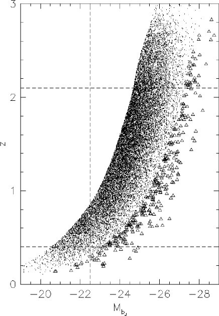
Figure 19: ($M_{\rm b_{\rm J}},z$) distribution for 2QZ (points) and 6QZ (triangles) QSOs. Dashed lines indicate the limits of our maximum likelihood analysis, $M_{\rm b_{\rm J}}<-22.5$ and $0.4<z<2.1$. For this plot we assume $\Omega_{\rm m}=0.3$, $\Omega_{\Lambda}=0.7$ and $H_{0}=70$km s^-1Mpc^-1.

Due to a number of different effects, the completeness near the edge of a 2dF field could be lower than in the central region. We therefore look at the completeness within a 2dF field as a function of radius from the field centre. We first take each individual observation of a 2dF field and find the spectroscopic completeness as a function of radius from the field centre. In Fig. 18 we plot the number weighted average of these completeness estimates (filled circles). A decline in completeness with increasing radius is visible at $>0.4^{\circ}$, with regions at $>0.9^{\circ}$ on average only $\sim 65$ per cent complete. This could be caused by a number of effects. Systematic errors in astrometry or field rotation would tend to be worse towards the edge of the 2dF field. Similarly, atmospheric refraction effects, if a field was observed at a different hour angle than it was configured for, would also be most noticeable at the edges of the field. In order to see how this radially dependent completeness affects the final 2QZ catalogue, we then derive the radially dependent completeness, using only the best observation of each object, and include objects that are within a given field, but actually observed in an overlapping field. This radial completeness estimate is also shown in Fig. 18 (open circles). When using only the best observations and including overlaps, we find that there is no significant decline in the completeness at large radii. This suggests that the final 2QZ catalogue should not be seriously affected by radially variable incompleteness. The most extreme test of the catalogue uniformity is in clustering analysis. We have performed detailed simulations of the radial completeness variations and their effect on the two-point correlation function, and confirm that these radial variations have negligible impact on the clustering analysis (Croom et al. 2003 in preparation). These tests also imply that any variation in completeness as a function of fibre number do not effect measurements of clustering.

4 The optical QSO luminosity function

4.1 Data

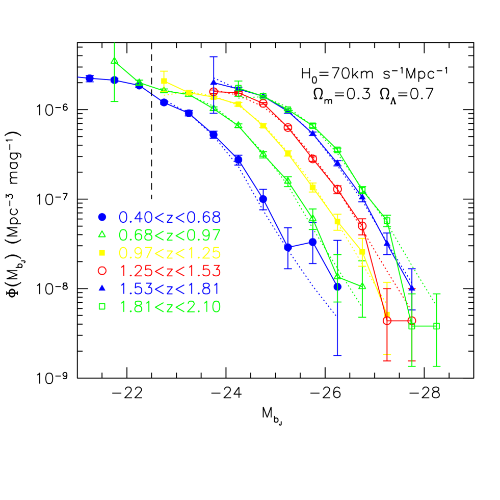
Figure 20: The optical QSO luminosity function for the 2QZ + 6QZ sample in six redshift intervals (open and filled points). The dotted lines denote the predictions of the best fit double power law exponential evolution model to dataset with $M_{\rm b_{\rm J}}<-22.5$ in the $\Lambda$ Universe. The model values are calculated based on the accessible volume in each bin, exactly as the data, and so contain an explicit correction for incomplete bins. This means that the dotted lines may not appear to follow an exact power law. The vertical dashed line indicates the $M_{\rm b_{\rm J}}<-22.5$ limit used in the maximum likelihood fitting.

Based on the discussion above, we chose to use the 2QZ sample defined by a minimum mean sector spectroscopic completeness of 70 per cent, and the full SGP declination strip for the 6QZ. The effective survey area corresponds to 595.9 deg² for the 2QZ and 333.0 deg² for the 6QZ after coverage correction. All QSO magnitudes and sector magnitude limits were corrected for galactic extinction on the basis of the mean extinction values [Schlegel et al. 1998] in each sector.

A strength of the combined 2QZ/6QZ data set is its homogeneous selection and photometry. With the statistical precision that the 2QZ/6QZ can provide, errors in the estimate of the QSO OLF are largely dominated by systematic effects (apart from possibly the very brightest luminosities). Therefore, although it is possible to combine other surveys, in the analysis below, we chose not to include QSOs from any other catalogue. We also limit the analysis to regions of the catalogue where the photometric completeness is greater than 85 per cent (see Fig. 10), corresponding to a redshift range $0.4<z<2.1$. In Fig. 19 we show the $z$ vs. $M_{\rm b_{\rm J}}$ distribution of sources, indicating the above cuts.

Within this redshift range, the corrections for photometric, morphological and spectroscopic completenesses derived above were then applied to this combined dataset. To minimize the noise on the estimate of the redshift-dependent spectroscopic incompleteness the estimates presented in Table 3 were block-averaged over $\Delta z=0.3$ bins.

4.2 $1/V$ estimator

As in Paper I, we first obtain a graphical binned representation of the OLF and its evolution with redshift using the $1/V$ estimator devised by Page & Carrera (2000). We chose to bin the OLF into six equally spaced linear redshift bins over the range $0.4<z<2.1$ and into $\Delta M_{\rm b_{\rm J}}=0.5$ bins in absolute magnitude. All bins that contain at least one QSO are plotted. However, it should be noted that bins near the magnitude limits of the survey can be biased even using the Page & Carrera estimator (see Paper I). This is the case if part of the bin lies outside of the survey limits, and there is significant evolution across the bin.

The resulting OLF, calculated for a flat universe with $\Omega_{\rm m}=0.3$, $\Omega_{\Lambda}=0.7$ and $H_{0}=70$km s^-1Mpc^-1 (which we call the $\Lambda$ cosmology) is plotted in Fig. 20. The value of the OLF, statistical error and the number and mean redshift of QSOs contributing to each plotted point in the figure is given in Table 4. We determine upper and lower 1$\sigma$ (84.13 per cent one-sided) confidence intervals for a Poisson distribution [Gehrels 1986] for bins which have small numbers of QSOs ($<20$), and hence have errors which are not well represented by $\sqrt{N}$ errors.

Table 4: Binned luminosity function estimate for $\Omega_{\rm m}=0.3$, $\Omega_{\Lambda}=0.7$ and $H_{0}=70$km s^-1Mpc^-1, as plotted in Fig. 20. We give the value of $\log\Phi$ in 6 redshift intervals, and in $\Delta M_{\rm b_{\rm J}}=0.5$ mag bins. We also list the mean redshift ($\bar{z}$) in each bin, the number of QSOs contributing to the OLF ($N_{\rm Q}$) and the lower and upper errors ($\Delta\log\Phi$).

	$0.40<z<0.68$					$0.68<z<0.97$					$0.97<z<1.25$
$M_{\rm b_{\rm J}}$	$\bar{z}$	$N_{\rm Q}$	$\log\Phi$	$\Delta\log\Phi$		$\bar{z}$	$N_{\rm Q}$	$\log\Phi$	$\Delta\log\Phi$		$\bar{z}$	$N_{\rm Q}$	$\log\Phi$	$\Delta\log\Phi$
–20.75	0.43	31	–5.62	–0.09	+0.07	–	0	–	–	–	–	0	–	–	–
–21.25	0.47	166	–5.65	–0.04	+0.03	–	0	–	–	–	–	0	–	–	–
–21.75	0.54	393	–5.67	–0.02	+0.02	0.69	2	–5.46	–0.45	+0.36	–	0	–	–	–
–22.25	0.57	484	–5.73	–0.02	+0.02	0.73	184	–5.70	–0.03	+0.03	–	0	–	–	–
–22.75	0.57	329	–5.92	–0.02	+0.02	0.80	553	–5.79	–0.02	+0.02	0.99	18	–5.68	–0.12	+0.11
–23.25	0.58	256	–6.04	–0.03	+0.03	0.84	710	–5.83	–0.02	+0.02	1.06	469	–5.81	–0.02	+0.02
–23.75	0.58	139	–6.28	–0.04	+0.04	0.84	513	–5.99	–0.02	+0.02	1.12	863	–5.86	–0.02	+0.01
–24.25	0.60	61	–6.56	–0.06	+0.05	0.86	340	–6.18	–0.02	+0.02	1.12	754	–5.94	–0.02	+0.02
–24.75	0.62	18	–7.00	–0.12	+0.11	0.87	155	–6.50	–0.04	+0.03	1.13	452	–6.18	–0.02	+0.02
–25.25	0.61	5	–7.54	–0.24	+0.22	0.88	62	–6.80	–0.06	+0.05	1.13	225	–6.49	–0.03	+0.03
–25.75	0.63	5	–7.48	–0.24	+0.22	0.86	18	–7.22	–0.12	+0.11	1.14	83	–6.87	–0.05	+0.05
–26.25	0.63	1	–7.98	–0.77	+0.52	0.80	4	–7.87	–0.28	+0.25	1.10	23	–7.25	–0.10	+0.08
–26.75	–	0	–	–	–	0.86	3	–7.98	–0.34	+0.29	1.16	10	–7.59	–0.16	+0.15
–27.25	–	0	–	–	–	–	0	–	–	–	1.17	2	–8.29	–0.45	+0.36
	$1.25<z<1.53$					$1.53<z<1.81$					$1.81<z<2.10$
$M_{\rm b_{\rm J}}$	$\bar{z}$	$N_{\rm Q}$	$\log\Phi$	$\Delta\log\Phi$		$\bar{z}$	$N_{\rm Q}$	$\log\Phi$	$\Delta\log\Phi$		$\bar{z}$	$N_{\rm Q}$	$\log\Phi$	$\Delta\log\Phi$
–23.75	1.34	468	–5.80	–0.02	+0.02	1.54	3	–5.70	–0.34	+0.29	–	0	–	–	–
–24.25	1.40	1103	–5.81	–0.01	+0.01	1.64	728	–5.77	–0.02	+0.02	1.84	26	–5.76	–0.09	+0.08
–24.75	1.41	897	–5.93	–0.01	+0.01	1.68	1142	–5.85	–0.01	+0.01	1.93	897	–5.85	–0.01	+0.01
–25.25	1.41	495	–6.20	–0.02	+0.02	1.68	823	–6.02	–0.02	+0.01	1.96	898	–6.00	–0.01	+0.01
–25.75	1.41	228	–6.55	–0.03	+0.03	1.68	470	–6.27	–0.02	+0.02	1.95	618	–6.18	–0.02	+0.02
–26.25	1.42	95	–6.89	–0.05	+0.04	1.69	224	–6.60	–0.03	+0.03	1.96	333	–6.45	–0.02	+0.02
–26.75	1.44	24	–7.30	–0.10	+0.08	1.71	82	–6.98	–0.05	+0.05	1.97	120	–6.90	–0.04	+0.04
–27.25	1.31	2	–8.36	–0.45	+0.36	1.72	16	–7.50	–0.12	+0.12	1.98	43	–7.24	–0.07	+0.06
–27.75	1.48	2	–8.36	–0.45	+0.36	1.71	5	–8.00	–0.24	+0.22	2.07	2	–8.42	–0.45	+0.36
–28.25	–	0	–	–	–	–	0	–	–	–	1.94	2	–8.42	–0.45	+0.36

4.3 Maximum likelihood analysis

To obtain a more quantitative descriptions of suitable models we carried out a maximum likelihood analysis, fitting a number of models to the data (e.g. Boyle, Shanks & Peterson 1988). This technique relies on maximizing the likelihood function $S$ corresponding to the Poisson probability distribution function for both model and data [Marshall et al. 1983]. Previously, we have used the 2D K-S statistic to provide a goodness-of-fit measure for ‘best fit’ maximum likelihood models. However, the data-set is now so large that the K-S test, notoriously insensitive to discrepancies between the data and the model predictions in the wings of the distributions, is very poor at discriminating between models. Instead, we choose to use the $\chi^{2}$ statistic, based on the numbers of observed and predicted QSOs in each of the $M_{\rm b_{\rm J}},z$ bins used for the $1/V$ estimator above.

In keeping with our general philosophy of previous maximum likelihood fits to the OLF, we used the minimum numbers of free parameters in any model required to obtain an acceptable fit. Our $a\ priori$ definition of an acceptable fit was one which could not be rejected at the 99 per cent confidence level or greater based on the $\chi^{2}$ statistic. Errors on the fit parameters correspond to the $\Delta S=1$ contours around each parameter, or, equivalently, the 68 per cent confidence contour for one interesting parameter.

While carrying out the maximum likelihood analysis, we employ an absolute magnitude limit $M_{\rm b_{\rm J}}>-22.5$ for the $\Lambda$ cosmology and $M_{\rm b_{\rm J}}>-22$ for an Einstein-de Sitter (EdS) cosmology ($\Omega_{\rm m}=1.0$, $\Omega_{\Lambda}=0.0$ and $H_{0}=70$km s^-1Mpc^-1). This absolute magnitude cut excludes AGN where the contribution from the host galaxy (either photometrically or spectroscopically) may lead to a significantly bias against the inclusion or identification of such objects in the 2QZ which is not accurately modelled by the above completeness analysis. The calculated absolute magnitude of these sources would also be biased by the inclusion of flux from the host galaxy.

Table 5: The best fit OLF model parameters from the maximum likelihood analysis for the range of models discussed. We list the redshift range and faint $M_{\rm b_{\rm J}}$ limit of the data fitted, the evolution model and cosmology used (assuming a flat $\Omega_{\rm m}+\Omega_{\Lambda}=1$ Universe), the number of QSOs in the analysis ($N_{\rm Q}$) and the best fit values of the model parameters. We also give the $\chi^{2}$ value for the comparison of the model to the data, as well as the number of degrees of freedom ($\nu$) and the $\chi^{2}$ probability.

Redshift	$M_{\rm b_{\rm J}}$	Evolution	$\Omega_{\rm m}$	$N_{\rm Q}$	$\alpha$	$\beta$	$M_{\rm b_{\rm J}}^{*}$	$k_{1}$	$k_{2}$	$\Phi^{*}$	$\chi^{2}$	$\nu$	$P_{\chi^{2}}$
range	limit	model								${\rm Mpc}^{-3}{\rm mag}^{-1}$
$0.4<z<2.1$	–22.5	$k_{1}z+k_{2}z^{2}$	0.3	15830	–3.31	–1.09	–21.61	1.39	–0.29	1.67$\times 10^{-6}$	71.1	62	2.00e-01
$0.4<z<2.1$	–22	$k_{1}z+k_{2}z^{2}$	1.0	15875	–3.28	–1.12	–20.74	1.49	–0.31	5.07$\times 10^{-6}$	148.6	61	2.88e-09
$0.4<z<2.1$	–22.5	$e^{k\tau}$	0.3	15830	–3.25	–1.01	–20.47	6.15	–	1.84$\times 10^{-6}$	64.5	63	4.24e-01
$0.4<z<2.1$	–22	$e^{k\tau}$	1.0	15875	–3.16	–0.98	–18.54	7.16	–	5.99$\times 10^{-6}$	148.6	62	2.52e-07

Table 6: The number of observed, $N_{\rm obs}$, and predicted, $N_{\rm pred}$ QSOs for the best fit exponential evolution model in $\Lambda$ Universe, along with the significance of the devation away from the model, $\sigma$.

	$0.40<z<0.68$			$0.68<z<0.97$			$0.97<z<1.25$			$1.25<z<1.53$			$1.53<z<1.81$			$1.81<z<2.10$
$M_{\rm b_{\rm J}}$	$N_{\rm obs}$	$N_{\rm pred}$	$\sigma$	$N_{\rm obs}$	$N_{\rm pred}$	$\sigma$	$N_{\rm obs}$	$N_{\rm pred}$	$\sigma$	$N_{\rm obs}$	$N_{\rm pred}$	$\sigma$	$N_{\rm obs}$	$N_{\rm pred}$	$\sigma$	$N_{\rm obs}$	$N_{\rm pred}$	$\sigma$
–22.75	329	354.13	–1.34	553	563.35	–0.44	18	12.47	1.20	–	–	–	–	–	–	–	–	–
–23.25	256	254.05	0.12	710	698.62	0.43	469	480.41	–0.52	0	0.42	–1.01	–	–	–	–	–	–
–23.75	139	134.55	0.38	513	546.66	–1.44	863	892.78	–1.00	468	490.51	–1.02	3	3.40	–0.23	–	–	–
–24.25	61	51.30	1.35	340	336.81	0.17	754	731.82	0.82	1103	1030.66	2.25	728	722.35	0.21	26	20.07	1.32
–24.75	18	13.40	0.97	155	160.39	–0.43	452	467.05	–0.70	897	821.93	2.62	1142	1151.22	–0.27	897	883.79	0.44
–25.25	5	4.68	0.10	61	55.87	0.69	225	233.01	–0.52	495	505.52	–0.47	823	839.19	–0.56	898	958.27	–1.95
–25.75	5	1.61	1.36	18	14.08	0.81	83	90.69	–0.81	228	243.56	–1.00	470	469.90	0.00	618	611.27	0.27
–26.25	1	0.45	0.27	4	4.98	–0.46	23	22.21	0.17	95	94.76	0.02	224	210.91	0.90	333	302.49	1.75
–26.75	0	0.05	–0.03	3	1.76	0.49	10	7.27	0.72	24	21.84	0.46	82	75.41	0.76	120	125.28	–0.47
–27.25	–	–	–	0	0.49	–1.03	2	2.59	–0.39	2	7.18	–1.98	16	16.59	–0.15	43	40.26	0.43
–27.75	–	–	–	0	0.04	–0.02	0	0.88	–1.16	2	2.56	–0.37	5	5.74	–0.32	2	9.49	–2.48
–28.25	–	–	–	–	–	–	0	0.11	–0.53	0	0.89	–1.16	0	2.04	–1.56	2	3.38	–0.79
–28.75	–	–	–	–	–	–	–	–	–	0	0.11	–0.51	0	0.69	–1.09	0	1.20	–1.28
–29.25	–	–	–	–	–	–	–	–	–	–	–	–	0	0.06	–0.08	0	0.38	–1.00
–29.75	–	–	–	–	–	–	–	–	–	–	–	–	–	–	–	0	0.01	0.00

4.4 Model fitting

Figure 21: Differential number-magnitude, $n(b_{\rm J})$, relation for the 2QZ (filled circles) and 6QZ (open circles) for QSOs with $0.4<z<2.1$ and $M_{\rm b_{\rm J}}<-22.5$. Also shown is the prediction from the best fit exponential evolution model in the $\Lambda$ Universe.

Figure 22: Observed number-redshift, $n(z)$, relation for the 2QZ survey for $0.4<z<2.1$ and $M_{\rm b_{\rm J}}<-22.5$. The solid line indicates the best fit exponential evolution model for the $\Lambda$ Universe.

Based on our previous results with the 2QZ, we chose to model the OLF $\Phi(L,z)$ as a double power law in luminosity such that

$$\Phi(L_{\rm b_{\rm J}},z)=\frac{\Phi(L_{\rm b_{\rm J}}^{*})}{(L_{\rm b_{\rm J}}/L_{\rm b_{\rm J}}^{*})^{-\alpha}+(L_{\rm b_{\rm J}}/L_{\rm b_{\rm J}}^{*})^{-\beta}}.$$ (10)

Expressed in magnitudes this becomes

$$\Phi(M_{\rm b_{\rm J}},z)=\frac{\Phi(M_{\rm b_{\rm J}}^{*})}{10^{0.4(\alpha+1)(M_{\rm b_{\rm J}}-M_{\rm b_{\rm J}}^{*})}+10^{0.4(\beta+1)(M_{\rm b_{\rm J}}-M_{\rm b_{\rm J}}^{*})}}.$$ (11)

The evolution of the luminosity function is given by the redshift dependence of the break luminosity $L_{\rm b_{\rm J}}^{*}\equiv L_{\rm b_{\rm J}}^{*}(z)$ or magnitude, $M_{\rm b_{\rm J}}^{*}\equiv M_{\rm b_{\rm J}}^{*}(z)$. In earlier papers in this series, we have modelled this evolution as a 2nd-order polynomial of the form

$$L_{\rm b_{\rm J}}^{*}(z)=L_{\rm b_{\rm J}}^{*}(0)10^{k_{1}z+k_{2}z^{2}},$$ (12)

or equivalently,

$$M_{\rm b_{\rm J}}^{*}(z)=M_{\rm b_{\rm J}}^{*}(0)-2.5(k_{1}z+k_{2}z^{2}).$$ (13)

In this paper we also attempt to fit an exponential evolution with look-back time ($\tau$) of the form

$$L_{\rm b_{\rm J}}^{*}(z)=L_{\rm b_{\rm J}}^{*}(0)\exp(k_{1}\tau).$$ (14)

Expressing this in magnitudes it becomes

$$M_{\rm b_{\rm J}}^{*}(z)=M_{\rm b_{\rm J}}^{*}(0)-1.08k_{1}\tau$$ (15)

Although such models with an exponential evolution in $\tau$ have previously been shown not to fit the QSO distribution [Boyle et al. 2000, La Franca & Cristiani 1997] for an EdS Universe, exponential evolution models have not been fitted to Universes with non-zero $\Omega_{\Lambda}$.

These models were fitted to the survey data for both EdS and $\Lambda$ cosmologies. The statistical errors on individual parameters are: $\sigma(\alpha)=0.05$, $\sigma(\beta)=0.1$, $\sigma(M_{\rm b_{\rm J}}^{*})=0.2$, $\sigma(k_{1})({\rm exponential})=0.1$, $\sigma(k_{1})({\rm polynomial})=0.03$, $\sigma(k_{2})({\rm polynomial})=0.01$. We note that the size of the 2QZ/6QZ sample is such that residual systematic uncertainties are likely to dominate the model fitting. The completeness analysis described above (Section 3) is aimed at minimizing such uncertainties. Although not affecting the shape of the fitted QSO OLF, any error in the survey $b_{\rm J}$ zero-point will translate to a shift in $M_{\rm b_{\rm J}}^{*}$. Checks against a small number of independent CCD sequences in the 2QZ region suggest that such an error must be no greater than 0.05 mag.

4.5 Results

We find that both the polynomial evolution in $z$ and the exponential evolution in $\tau$ provide acceptable fits when using the $\Lambda$ cosmology. The best fit model values are shown in Table 5, along with their derived $\chi^{2}$ values and probability of acceptance. The best fit exponential model using the $\Lambda$ cosmology has a rate of evolution defined by $k_{1}=6.15$. This corresponds to an ’e-folding’ time of approximately 2Gyr. Both evolutionary models provide a poor fit to the full data set in an EdS Universe. Although these model fits are rejected, for completeness we also show the best fit model parameters for an EdS Universe in Table 5.

The predicted differential number-magnitude, $n(b_{\rm J})$, and number-redshift, $n(z)$, relations for the 2QZ and 6QZ surveys based on the best fit exponential evolution model in a $\Lambda$ Universe are shown in Fig. 21 and Fig. 22. The model predictions provide a good fit to the derived $n(b_{\rm J})$ and observed $n(z)$ relations for QSOs over the redshift range $0.4<z<2.1$ and with absolute magnitudes $M_{\rm b_{\rm J}}<-22.5$. The model also provides a good match to the binned OLF (see Fig. 20), although some small differences can be seen. In Fig. 20 the model points are derived based on the accessible volume in each bin (as for the data points). This adjusts the model for biases introduced by binning in exactly the same way as the data. As a result, the model curves (dotted lines) do not trace out perfect double power laws, although they are based on the double power law model.

To investigate any systematic deviations of the data away from the model we show the number of objects observed and predicted, and the significance of the difference between the two, $\sigma=(N_{\rm obs}-N_{\rm pred})/\sqrt{N_{\rm pred}})$ in Table 6 for the exponential model in a $\Lambda$ Universe. Positive values of $\sigma$ correspond to cases in which there are more QSOs observed than predicted. $\sqrt{N_{\rm pred}}$ is only a reasonable estimate of the error for large $N_{\rm pred}$. For small $N_{\rm pred}$ ($<20$) we use the 84.13 per cent one-sided confidence interval in a Poisson distribution to determine the error. As the Poisson distribution is not a symmetric function, we choose the error estimate depending which side of the model expectation the observed number of QSOs lies. While not giving the formally correct significance for an arbitrary number of standard devations (as the Poisson distribution still has a different shape to a Gaussian distribution) this method does produce a more realistic estimate of how significant the deviations from the model are.

It is clear from Fig. 20 and Table 6 that although the model is in general good agreement with the data, there are some deviations away from the model. The most significant of these are at relatively faint magnitudes near the break in the OLF (e.g. at $M_{\rm b_{\rm J}}\sim-24.0$ in the $1.25<z<1.53$ interval). Although the deviations are small, these bins contain large numbers of QSOs, making the errors on each bin small. It is possible that the simple double power law parameterization is not a perfect description of the data when sufficient statistical precision is available. It is also possible that residual systematic errors are beginning to dominate the fitting. As a second goodness of fit test we also calculate the 2-D K-S probability for the exponential model in the $\Lambda$ cosmology, and find a value of $6.4$ per cent, making this model acceptable at the $2\sigma$ level and under our pre-defined criteria (models should not be rejected at $>99$ per cent level). At the bright end of the OLF there is some evidence of the steepening of the bright end slope towards higher redshift found by other authors (e.g. Goldschmidt & Miller 1998), with the model slightly under-prediciting the number of bright low redshift QSOs and similarly over-prediciting the numbers of bright high redshift QSOs. By simply examining the numbers observed and predicited we find there is a $2\sigma$ excess of QSOs in our lowest redshift bin at $M_{\rm b_{\rm J}}<-24.0$ (90 observed vs. 71.49 predicted), and a $1\sigma$ deficit of QSOs in our highest redshift bin at $M_{\rm b_{\rm J}}<-27.0$ (47 observed vs. 54.72 predicited). We note that these deviations from the model are less significant than the those found at fainter magnitudes, discussed above.

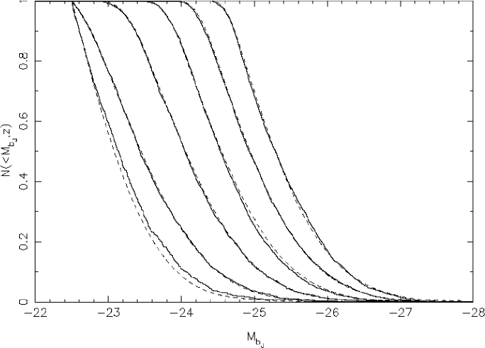
Figure 23: The normalized cumulative distribution of QSOs in each of our six redshift intervals (solid lines) going from low (left) to high (right) redshift. These are the raw observed numbers limited to $M_{\rm b_{\rm J}}<-22.5$ in the $\Lambda$ cosmology. Also plotted are the predicted cumulative distributions from the best fit exponential evolution model (dashed lines) after correcting them for incompleteness.

To further examine deviations from the best fit model we carry out an analysis similar to Goldschmidt & Miller (1998). We compare the cumulative distribution of the number of QSOs observed and predicted as a function of $M_{\rm b_{\rm J}}$ for our six separate redshift slices. This test has the advantage of not relying on comparisons to binned luminosity functions. Both the data (solid lines) and models (dashed lines) are shown in Fig 23. We use the best fit model using the exponential evolution in look-back time in a $\Lambda$ cosmology. Both the model and data are limited to $M_{\rm b_{\rm J}}<-22.5$ in order to compare only the regions fitted. We see that there is good general agreement between the model and data. However, we do see that the data in the lowest redshift interval ($0.40<z<0.68$) contains more bright QSOs than predicted by the model. We carry out a 1D K-S test comparing the model and data in each of our six redshift slices. The resulting probabilities of the null hypothesis that the data are drawn from a distribution described by the model are 0.037, 0.725, 0.708, 0.068, 0.806, 0.099 for the low to high redshift intervals respectively. The largest deviation is found in the lowest redshift interval, in which the data deviate from the model at the $\sim 2\sigma$ level. This agrees with the excess found by examining the numbers of predicted and observed low redshift QSOs at $M_{\rm b_{\rm J}}<-24$ and is further evidence of the excess of bright low redshift QSOs found by other authors (e.g. Goldschmidt & Miller 1998). If we examine the binned OLF in Fig. 20, we see that the excess over the model appears to occur at intermediate magnitudes, $M_{\rm b_{\rm J}}\sim-24.0$ and brighter.

We also test the effect of extending the range of our fits in both absolute magnitude and redshift. When fitting the exponential evolution model in a $\Lambda$ cosmology we obtain an acceptable fit with a faint limit of $M_{\rm b_{\rm J}}<-22$ rather than our adopted limit of $M_{\rm b_{\rm J}}<-22.5$, with parameters virtually indistinguishable from the best fit values shown in Table 5 for the $M_{\rm b_{\rm J}}<-22.5$ limit. Extending the redshift range of our fits we find that acceptable fits to the exponential evolution model in a $\Lambda$ cosmology are found in the redshift range $0.4<z<2.2$, but not at higher redshift (e.g. $0.4<z<2.3$). Similar results are found with the polynomial evolution model, with an acceptable fit at $0.4<z<2.2$, but not with $0.4<z<2.3$. This is indicative of either (or both) a change in the evolution of QSOs or (and) possible residual systematic errors in the large completeness corrections required at high redshift.

This appears to demonstrate that a sample of the size of the 2QZ is limited by the accuracy of corrections for systematic imcompleteness, rather than random noise. It is also very likely that although the simple model fits above provide a good general description for the evolution of the QSO population, the actual QSO luminosity function, including its evolution, has a more complex form. Evolution in the QSO OLF appears to turn over, peaking at $z\sim 2-3$, with declining QSO activity at higher redshift (e.g. Warren, Hewett & Osmer 1994; Fan et al. 2001). There are a number of further analyses that could be carried out on the QSO OLF, however we leave these to future papers.

The physical mechanisms which drive the shape and evolution of the QSO OLF are still uncertain. The two power law model fits the data well, but the observed break may be due to a number of phenomena. The break in the OLF could correspond to a break in the black hole mass function, which in turn is related to the mass (or velocity dispersion) of the host galaxy. Black hole mass is seen to correlate well with the velocity dispersion of the spheroidal component of local galaxies (e.g. Gebhardt et al 2000), although this has yet to be observed at high redshift. However, the correlation between host galaxy and AGN luminosity is less clear with only a weak correlation with large scatter found between the two (e.g. Schade et al. 2000), at least at low redshift. This implies that AGN have a broad range of efficiencies, with some accreting near (or above) the Eddington limit and others accreting at a much lower rate. Such a broad range in accretion rates convolved with any black hole mass function would contrive to significantly blur any break. However, it is likely, although by no means certain, that only a small fraction of sources accrete at super-Eddington rates. This then provides a second natural cut off at high luminosity. In this context we also need to understand the cause of the strong luminosity evolution seen in the QSO population. One view is that this is driven by a decline in accretion rate towards low redshift, as the available fuel becomes more scarce. A second factor, is that possible tiggering events (e.g. mergers) are more common at high redshift. The current simple semi-analytic models of QSO formation (e.g. Kauffmann & Haehnelt 2000) predict that black hole masses will be lower at high redshift, but that these AGN will be accreting closer to the Eddington limit. This implies that for a given luminosity, black hole masses will be lower at high redshift. This model is called into question by the observation of no correlation between QSO line widths (which should provide an estimate of black hole mass) and redshift [Corbett et al. 2003]. It is clear that the QSO OLF, along with other observations of black hole mass estimates and host galaxy properties have the ability to help us understand the underlying physics driving AGN formation and evolution.

The 2QZ and 6QZ surveys are being made available to the astronomical community. It is hoped that they will provide a valuable and lasting resource for astronomers, and allow greater insight into the physical processes governing AGN as well as enhancing our understanding of cosmology and the structure of the Universe at high redshift.

This paper has been produced using the Blackwell Scientific Publications TeXmacros.

References

- [Bailey et al. 2003] Bailey J., Glazebrook K., Offer A., Taylor K., 2003, MNRAS submitted
- [Bailey & Glazebrook 1999] Bailey J., Glazebrook G., 1999, 2dF User Manual, Anglo-Australian Observatory
- [Becker et al. 1995] Becker R. H., White R. L., Helfand D. J., 1995, ApJ, 450, 559
- [Bennett et al. 2003] Bennett C. L. et al., 2003, ApJ submitted (astro-ph/0302207)
- [Boyle et al. 2000] Boyle B.J., Shanks T., Croom S.M., Smith R.J., Miller L., Loaring N., Heymans C., 2000, MNRAS, 317, 1014
- [Boyle et al. 1988] Boyle B.J., Shanks T., Peterson B.A., 1988, MNRAS, 235, 935
- [Brotherton et al. 1998] Brotherton M.S., van Breugel W., Smith R.J., Boyle B.J., Shanks T., Croom S.M., Miller L., Becker R.H., 1998, ApJL, 505, 7
- [Colless et al. 2001] Colless et al., 2001, MNRAS, 328, 1039
- [Condon et al. 1998] Condon J.J., Cotton W.D., Greisen E.W., Yin Q. F., Perley R.A., Taylor G.B., Broderick J.J., 1998, AJ, 115, 1693
- [Corbett et al. 2003] Corbett E.A., 2003, MNRAS, 343, 705
- [Croom et al. 2002] Croom S.M. et al., 2002, MNRAS, 337, 275
- [Croom et al. 2001a] Croom S. M., Shanks T., Boyle B. J., Smith R. J., Miller L., Loaring N., Hoyle F., 2001a, MNRAS, 325, 483
- [Croom et al. 2001b] Croom S. M., Smith R. J., Boyle B. J., Shanks T., Loaring N. S., Miller L., Lewis I. J., 2001b, MNRAS, 322, L29
- [Croom 1997] Croom S.M., 1997, PhD Thesis, University of Durham
- [Fan et al. 2001] Fan X. et al., 2001, AJ, 122, 2833
- [Francis et al. 1991] Francis P. J., Hewett P. C., Foltz C. B., Chaffee F. H., Weymann R. J., Morris S. L., 1991, ApJ, 373, 465
- [Gebhardt et al. 2000] Gebhardt K. et al., 2000, ApJ, 539, L13
- [Gehrels 1986] Gehrels N., 1986, ApJ, 303, 336
- [Goldschmidt & Miller 1998] Goldschmidt P., Miller L., 1998, MNRAS, 293, 107
- [Hambly et al. 2001] Hambley N.C. et al., 2001, MNRAS, 326, 1279
- [Hawkins & Veron 1995] Hawkins M.R.S., Veron P., 1995, MNRAS, 275, 1102
- [Hewett et al. 1993] Hewett P.C., Foltz C.B., Chaffee F.H., 1993, ApJ, 406, L43
- [Hewett et al. 1995] Hewett P.C., Foltz C.B., Chaffee F.H., 1995, AJ, 109, 1498
- [Hewett et al. 2001] Hewett P.C., Foltz C.B., Chaffee F.H., 2001, AJ, 122, 518
- [Hoyle et al. 2002] Hoyle F., Outram P.J., Shanks T., Boyle B.J., Croom S.M., Smith R.J., 2002, MNRAS, 332, 311
- [Kauffmann & Haehnelt] Kauffmann G., Haehnelt M., 2000, MNRAS311, 576
- [La Franca & Cristiani 1997] La Franca F., Cristiani S., 1997, AJ, 113, 1517
- [Lemon, Driver & Cross 2001] Lemon D., Driver S., Cross N., 2001, in Clowes R., Adamson A., & Bromage G. eds., The New Era of Wide Field Astronomy, ASP Conference Series 232, ASP, San Francisco, p 193
- [Lewis et al. 2002] Lewis I.J. et al., 2002, MNRAS, 333, 279
- [Londish et al. 2002] Londish D. et al., 2002, MNRAS, 334, 941
- [Marsh et al. 2002] Marsh T. R. et al., 2002, in G nsicke B.T., Beuermann K. & Reinsch K. eds., The Physics of Cataclysmic Variables and Related Objects, ASP Conference Series 261, ASP, San Francisco, p 200
- [Marshall et al. 1983] Marshall H.L., Tananbaum H., Avni Y., Zamorani G., 1983, ApJ, 269, 35
- [Meyer et al. 2001] Meyer M.J., Drinkwater M.J., Phillipps S., Couch W.J., 2001, MNRAS, 324, 343
- [Meyers et al. 2003] Meyers A. D., Outram P. J., Shanks T., Boyle B. J., Croom S. M., Loaring N. S., Miller L., Smith R. J., 2003, MNRAS, 342, 467
- [Miller et al. 2003] Miller L., Lopes A. M., Smith R. J., Croom S. M., Boyle B. J., Shanks T., Outram P.J., 2003, MNRAS submitted
- [Norberg et al. 2002] Norberg P. et al., 2002, MNRAS, 336, 907
- [Outram et al. 2003] Outram P. J., Hoyle F., Shanks T., Croom S. M., Boyle B. J., Miller L., Smith R. J., Myers A. D., 2003, MNRAS, 342, 483
- [Outram et al. 2001] Outram P.J. Hoyle F., Shanks T., Boyle B.J., Croom S.M., Loaring N.S., Miller L., Smith R.J., 2001, MNRAS, 328, 174
- [Page & Carrera 2000] Page M.J., Carrera F.J., 2000, MNRAS, 311, 433
- [Schade et al. 2000] Schade D. J., Boyle B. J., Letawsky M., 2000, MNRAS, 315, 498
- [Schlegel et al. 1998] Schlegel D.J., Finkbeiner D.P., Davis M., 1998, ApJ, 500, 525
- [Smith 1998] Smith R.J., 1998, Ph.D. Thesis, University of Cambridge
- [Smith et al. 2003] Smith R.J., Croom S.M., Boyle B.J., Shanks T., Miller L., Loaring N.S., 2003, MNRAS submitted.
- [Stoughton et al. 2002] Stoughton C. et al., 2002, AJ, 123, 485
- [Trèvese & Vagnetti 2002] Trèvese D., Vagnetti F., 2002, ApJ, 564, 614
- [Vanden Berk et al. 2001] Vanden Berk D. E. et al., 2001, AJ, 122, 549
- [Vennes et al. 2002] Vennes S., Smith R. J., Boyle B. J., Croom S. M., Kawka A., Shanks T., Miller L., Loaring N., 2002, MNRAS, 335, 673
- [Véron-Cetty & Véron 2000] Véron-Cetty M.P., Véron P., 2000, Quasars and Active Galactic Nuclei (9th Ed.).ESO Sci. Rep., 19, 1
- [Voges et al. 1999] Voges W. et al., 1999, AA, 349, 389
- [Voges et al. 2000] Voges W. et al., 2000, IAUC, 7432
- [Warren et al. 1991] Warren S. J., Hewett P. C., Irwin M. J., Osmer P. S., 1991, ApJS, 76, 1
- [Warren et al. 1994] Warren S. J., Hewett P. C., Osmer P. S., 1994, ApJ, 421, 412
- [Watson & Parker 1994] Watson F.G., Parker Q.A., 1994, in Crawford D.L., Craine E.R., eds., Instrumentation in Astronomy VIII, Proc. SPIE Vol. 2198, 65
- [Watson et al. 2000] Watson F.G., Parker Q.A., Bogatu G., Farrell T.J., Hingley B.E., Miziarski S., 2000, in Iye M., Moorwood A.F., eds., Optical and IR Telescope Instrumentation and Detectors, Proc. SPIE Vol. 4008, 123
- [Willis, Hewett & Warren 2001] Willis J. P., Hewett P. C., Warren S. J., 2001, MNRAS, 325, 1002
- [York et al. 2000] York D.G. et al., 2000, AJ, 120, 1579