An XMM-Newton study of the RGH 80 galaxy group

We present an X-ray study of the galaxy group RGH 80, observed by XMM-Newton. The X-ray emission of the gas is detected out to $\sim 462h^{-1}_{50}$ kpc, corresponding to $\sim 0.45r_{200}$. The group is relatively gas rich and luminous with respect to its temperature of $1.01\pm 0.01$ keV. Using the deprojected spectral analysis, we find that the temperature peaks at $\sim 1.3$ keV around $0.11r_{200}$, and then decreases inwards to 0.83 keV at the center and outwards to $\sim 70\%$ of the peak value at large radii. Within the central $\sim 60$ kpc of the group where the gas cooling time is less than the Hubble time, two-temperature model with temperatures of 0.82 and 1.51 keV and the Galactic absorption gives the best fit of the spectra, with $\sim 20\%$ volume occupied by the cool component. We also derive the gas entropy distribution, which is consistent with the prediction of cooling and/or internal heating models. Furthermore, the abundances of O, Mg, Si, S, and Fe decrease monotonically with radius. With the observed abundance ratio pattern, we estimate that $\sim 85\%$ or $\sim 72\%$ of the iron mass is contributed by SN Ia, depending on the adopted SN II models.

1 Introduction

In the past decade X-ray imaging spectroscopy has become a powerful probe of the physical conditions of the hot ($T^{>}_{\sim}10^{7}$ K) intergalactic medium (IGM) of galaxy groups. Spatial distributions of gas temperature, density and metallicity, as well as the structures of the gravitational potential and dark matter halos have been measured for numerous galaxy groups. This improves significantly our knowledge of dynamical properties and formation of galaxy groups. Among these, the discovery of similarity breaking of some IGM properties from clusters to groups is crucial for the study of cosmic evolution of the hot IGM in very massive halos of the universe. The well-known example is the deviation of the X-ray luminosity ($L_{\rm X}$) and temperature ($T$) relation of groups and clusters from the prediction of self-similar model (e.g. Edge & Stewart 1991; David et al. 1993; Wu, Xue & Fang 1999; Helsdon & Ponman 2000; Xue & Wu 2000 and references therein). The break lends strong support to the argument that the IGM of groups was much more affected by non-gravitational processes, such as radiative cooling and/or feedback of star formation, than the IGM of clusters. Another example is the detection of entropy excess in clusters and groups (Ponmam, Cannon & Navarro 1999; Lloyd-Davies, Ponman & cannon 2000; Xu, Jin & Wu 2001), which reinforces the presence of strong non-gravitational effects especially in the inner regions of poor clusters and groups. The reliable $L_{\rm X}-T$ relations and the entropy profiles obtained from spatially resolved X-ray imaging spectroscopy may allow one for the first time to distinguish between the competing non-gravitational models (Voit et al. 2002, 2003; Mushotzky et al. 2003).

X-ray spectra of groups are dominated by emission line features. The wealth of characteristic emission lines provides a robust tool for understanding the metal enrichment processes in the IGM and possibly for constraining the supernova history of galaxy groups (e.g. Finoguenov & Ponman 1999). However, an accurate determination of the metal abundances depends strongly on precise measurements of the temperature structure of the hot IGM in groups, as the dominated Fe L-shell lines are highly temperature sensitive (e.g. Buote 2002; Buote et al. 2003a). The high spectral resolution of XMM-Newton allows us to obtain the abundances of O and Mg in addition to Si, S and Fe, and provides us a deep insight into the chemical evolution history of groups with the abundance ratio pattern and the metal mass to light ratios (e.g. Xu et al. 2002; Matsushita, Finoguenov & Böhringer 2003).

In this paper, we report the results from new XMM-Newton observations of RGH 80, which was first identified by Ramella, Geller & Huchra (1989) in the center for astrophysics redshift survey. It was identified as an extended X-ray source in the ROSAT All-Sky Survey with an X-ray luminosity of $3.33\times 10^{43}h^{-2}_{50}$ erg s^-1 in the 0.1–2.4 keV band within an aperture of $1.0h^{-1}_{50}$ Mpc (NRGs241; Mahdavi et al. 2000). Global fitting of the ASCA SIS and GIS data by Davis, Mulchaey & Mushotzky (1999) yielded a mean gas temperature of $1.02\pm 0.05$ keV, an average abundance of $0.26^{+0.16}_{-0.08}Z_{\odot}$ for the $\alpha$ elements and $0.20^{+0.05}_{-0.06}Z_{\odot}$ for iron. However, Buote (2000) pointed out that a two-temperature spectral model provides a better fit to the ASCA spectra of RGH 80 and has a metallicity that is substantially higher than that obtained by the single temperature spectral model, $Z=0.67^{+0.42}_{-0.24}Z_{\odot}$. We will use the XMM-Newton data to examine the spatially resolved X-ray properties of the group and explore their physical applications.

In section 2, we describe the observations and data reduction procedure. We present the detailed spectral analysis in section 3. In Section 4 and 5, we derive the gas density profiles, and calculate the three dimensional distributions of gas and dark matter, respectively. We discuss and summarize the implications of our results in section 6 and 7. Throughout this paper, we take $H_{0}=50$ km s^-1 Mpc^-1, $\Omega_{\rm M}=1$ and $\Omega_{\Lambda}=0$. At the group redshift of 0.037, $1\arcmin$ corresponds to 60.2 kpc. Unless stated otherwise, we adopt $68\%$ confidence limit for error analysis.

2 Observation and data preparation

RGH 80 was observed with XMM-Newton for $\sim 33$ ks in revolution 563 on January 5th, 2003. The two MOS-CCD cameras were operated in full frame mode, and the pn-CCD camera was operated in extended full frame mode. All cameras were covered with the Thin1 filter. We generated the calibrated events lists for the data by using the tasks emchain and epchain that are packaged in the XMM SAS v5.4.1 software. In the analysis, we keep the events with PATTERNs 0–12 for the MOS cameras, and the events with PATTERNs 0–4 for the pn camera.

The EPIC background is mainly composed of solar soft protons, cosmic rays, and cosmic X-ray photon background (Lumb et al. 2002; Read & Ponman T.J. 2003). The background induced by soft protons is time variable, and hence causes large variations of intensity (flares) in the light curves. It can be subtracted by discarding those flare periods. Since in the very high energy band the effective area of XMM is negligible and the emission is dominated by the particle background, we extract the light curves in the energy band of 10–12 keV and 10–15 keV for the MOS and pn data, respectively, in 100s bins. An inspection of the light curves does not reveal any strong temporal variations. In order to determine the mean count rate and its error ($\sigma$) for the quiescent periods, we recursively clean the light curve by rejecting those time intervals during which the counts are $3\sigma$ outside the mean value, until the mean counts remain constant. We then define the thresholds at the $\pm 3\sigma$ level, and reject any time intervals outside these thresholds. After applying this screening criterion, the final useful exposures are 33.0 ks for MOS1, 32.7 ks for MOS2, and 26.6 ks for pn, respectively.

We utilize the EPIC blank sky event files available from the XMM calibrations (Lumb 2002) to represent the remaining quiescent background, which is mainly composed of the cosmic X-ray background and the background induced by cosmic rays. We applied the same PATTERN selection and light curve screening criteria as have been used above to the blank sky events. Since some internal background fluorescence lines show strong spatial inhomogeneities, such as Al K and Si K fluorescent lines in the MOS cameras (Lumb et al. 2002; Read & Ponman 2003) and Cu K fluorescent lines in the pn camera (Freyberg, Pfeffermann & Briel 2001; Lumb et al. 2002; Read & Ponman 2003), we use the skycast script to cast the background files into the corresponding sky coordinates of the source observations to ensure that the products of the background and the source are extracted from the same location.

Before subtracting the background, we first correct the vignetting effect for both source and background data sets with the SAS task evigweight, which computes a weight coefficient for each photon by using the inverse of the ratio of the effective area at the photon position and energy to the central effective area at the same energy.

In this paper, we follow the method of background subtraction as proposed by Arnaud and collaborators (cf. Arnaud et al. 2001; Pratt, Arnaud & Aghanim 2001; Arnaud et al. 2002; Majerowicz, Neumann & Reiprich 2002). Because the cosmic ray background varies from observation to observation by $\sim 10\%$, we normalize the background level of the blank sky files to that of the source observations. The ratios of the total count rates of the source observations to those of the blank sky data sets, extracted in the whole FOV of each camera in the energy band of 10–12 keV for the MOS data and 10–15 keV for the pn data, are adopted as the background normalization factors. They are 1.02, 1.00 and 0.96 for MOS1, MOS2 and pn respectively, for this observation.

The difference in the soft spectral component of the cosmic X-ray background between the source region and the blank field is investigated as follows. We first accumulate spectra in the annular region of 10–12$\arcmin$ for both source and blank sky data sets. This region is centered on the emission centroid of the group, and is located outside the group region. The emission centroid is computed within a $2.5\arcmin$ radius. Then we subtract the normalized blank sky spectrum from the source spectrum to obtain a residual background spectrum, which is subsequently subtracted from the spectrum of the group after rescaling its level according to the size of the area where the group spectrum is extracted.

We generate the on-axis ancillary response files (ARFs) using SAS task arfgen, and adopt the redistribution matrix files (RMFs) m11_r7_im_all_2002-11-07.rmf, m21_r7_im_all_2002-11-07.rmf and epn_ef20_sdY9.rmf for MOS1, MOS2 and pn respectively.

Following the standard method , we have corrected the out-of-time events of the pn data by a factor of 0.0232.

We show the vignetting corrected 0.5–3.0 keV image in Figure 1, which is produced by adaptively smoothing the combined exposure-corrected MOS1 and MOS2 image. We find that the X-ray emission of the group is extended and almost symmetric, except that it is contaminated by several fairly bright sources at 3.5–$6.5\arcmin$ from the group center. We then use SAS task edetect_chain to perform source detections in five energy bands (i.e., 0.2–0.5, 0.5–2.0, 2.0–4.5, 4.5–7.5, and 7.5–12.0 keV) and determine the source sizes following Katayama et al. (2002), which is described below. We divide the whole FOV into 8 annular regions centered at the centroid of the group emission, and extract an image for each region. The images are binned with a bin size of 40 pixels, and smoothed with a maximum gaussian smoothing size of $\sigma=5$ pixels. For each annular region, the average count rate per pixel and its error ($\sigma$) are found by recursively excluding the pixels with count rate $4\sigma$ above the mean value from the image until the mean count rate per pixel converges at a constant. Finally, for each source detected by edetect_chain except for the group, we determine its size, within which the count rate is $4\sigma$ higher than the mean value. The size of the point sources determined by this method is $\sim 20\arcsec$. We mask out all the sources in our further analysis for both source and blank sky data sets.

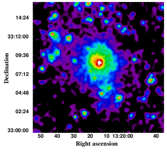
Figure 1: Vignetting corrected MOS image of RGH 80 in the 0.5–3.0 keV energy band, adaptively smoothed with a signal to noise ratio of 10 and a maximum gaussian smoothing size of $\sigma=5$ pixels.

3 Spectral analysis

While the diffuse X-ray emission of RGH 80 extends to a radius of $4.16\arcmin$ at $3\sigma$ level, the spectra in region $4.16\arcmin<r<7.67\arcmin$ still show strong features of a $\sim 0.95$ keV plasma. We therefore include this region in the spectral analysis. We extract spectra for a series of annuli centered at the centroid of the group emission in such a way that for each annulus, with a width larger than $30\arcsec$ (PSF consideration), the MOS spectrum has at least 3000 source counts in the 0.4–5.0 keV band to give a robust constraint on elemental abundances and gas temperatures. Finally, we obtain a total of four radially binned spectra for each camera (see Table 1 for details). The contribution from the source to the total count rate ranges from $\sim 97\%$ for the innermost spectrum to $\sim 20\%$ for the outermost one. The spectra are then grouped so that each bin has at least 20 counts, thereby allowing $\chi^{2}$ statistics to be used. We use XSPEC version 11.2.0 (Arnaud 1996) to analyze the spectra with one or two photoelectrically absorbed VAPEC spectral components (Smith et al. 2001) by fixing the hydrogen column density at the Galactic value ($1.05\times 10^{20}$ atom cm^-2; Dickey & Lockman 1990). For the spectra of the central region, more complicated spectral models such as cooling flow models are also examined. We adopt the solar abundances from Anders & Grevesse (1989) with Fe/H$=4.68\times 10^{-5}$ by number, which is 1.45 times larger than the meteoritic value. We have taken this difference into account when comparing with other studies. We divide the elements into six groups, i.e., O and Ne; Mg; Si; S and Ar; Fe and Ni; and the others (see also Finoguenov, Arnaud & David 2001). In group 1–5, the metal abundances in the same group are tied to each other and are set free in the spectral fittings. In group 6, metal abundances are fixed at the solar values. We perform a joint fit to the MOS1, MOS2 and pn spectra with the same model and model parameters, only allowing the normalization of each spectrum to vary independently.

Table 1: Quality of deprojected spectral fits

	R	1T		2T
shell	(arcmin)	$\chi^{2}$	dof	$\chi^{2}$	dof
1	0.00-0.58	335	273	230	271
2	0.58-1.67	260	280	219	278
3	1.67-4.08	237	320	230	318
4	4.08-7.67	422	371

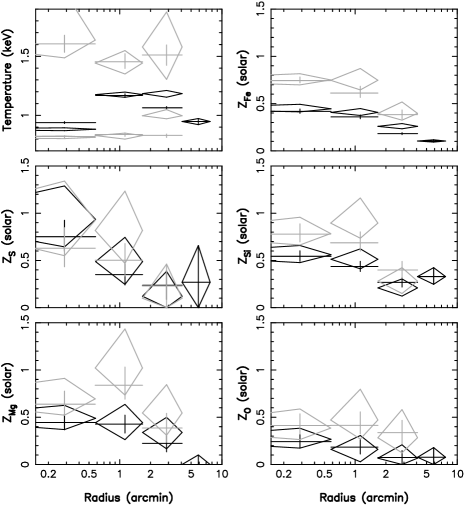
Figure 2: The deprojected (diamonds) and projected (crosses) temperature and abundance profiles and $1\sigma$ errors for the 1T (black) and 2T (gray) models. The emission measures of the hot and cool components of the 2T model are displayed in Figure 6.

3.1 Deprojection

With the standard “onion peeling” technique, we calculate the deprojected spectra by subtracting the emission projected from the outer shells, assuming that the spectral shape within each shell is the same and that the surface brightness profile is described by a $\beta$ model with $\beta=0.45$ and $r_{\rm c}=0.2\arcmin$, as will be shown in § 4.1. In order to take the contribution from beyond the outermost shell into account, we assume that the spectrum therein has the same shape as the one in the outmost shell and has the intensity proportional to the surface brightness of that region (e.g. Matsushita et al. 2002). Note that the deprojection analysis will propagate the errors of outer shells to inner ones. Therefore, the errors of deprojected spectra will become larger than those of the corresponding projected ones. The reduced chi-squared values of the deprojected spectral fitting become smaller than unity in most cases accordingly (see Table 1). In what follows We will mainly focus on the analysis of the deprojected spectra to obtain the three dimensional X-ray properties of the group.

3.2 Radial temperature & abundance profile

3.2.1 Single temperature fits

First we examine the deprojected spectra with a simple single-temperature VAPEC model (1T). The best-fit results are summarized in Figure 2 with black diamonds and in Table 1. We find that the temperature increases from $\sim 0.88$ keV at the center to $\sim 1.18$ keV at 0.6–4$\arcmin$, and then decreases to $\sim 0.95$ keV at large radii. Meanwhile, all the metal abundances decrease monotonically with radius, expect for the Si abundance in the outermost region that may have been biased by contamination of the background. In particular, the profile of the S abundance shows a steeper gradient: From the center to the outer regions, $Z_{\rm S}/Z_{\rm Fe}$ drops from 2.10 solar to 0.46 solar. This relatively higher enrichment of S around the center was also found in M 87 with XMM-Newton (Matsushita et al. 2003) and in the group NGC 1550 with $\it Chandra$ (Sun et al. 2003). Within $7.67\arcmin$, the emission weighted temperature is $1.01\pm 0.01$ keV, and the average iron abundance is $0.20\pm 0.01Z_{\odot}$, which are in good agreement with the previous ASCA results ($kT=1.02\pm 0.05$ keV, Fe$=0.20^{+0.05}_{-0.06}Z_{\odot}$; Davis et al. 1999).

It can be seen from Table 1 that the fitting of the best-fit 1T model is good for shells 2–4 while becomes much worse for the innermost region. As shown in Figure 3, the poor fit is due to the large residuals at 0.7–1.2 keV and at above 2.5 keV where the model predictions are apparently below the observed data. The former is mainly caused by the excess Fe L emissions, which implies the existence of cooler gas, and the latter indicates that there should be a harder spectral component. This suggests the need for a multiphase IGM model (cf. Buote 2000, 2002; Buote et al. 2003a).

We have also made an attempt to fit the projected spectra with the 1T model and plotted the results in Figure 2 with black crosses. In terms of the derived gas temperature and metal abundances the difference between the projected and deprojected results is only minor, with the deprojected analysis giving slightly larger abundances ($\sim 10\%$) for most cases.

Figure 3: MOS (lower crosses) and pn (upper crosses) spectra for annulus 1 fitted with the 1T (left panel) and 2T (right panel) models.

3.2.2 Two temperature fits

In order to improve the fits to the observed spectra, we employ a multiphase gas model by adding another thermal spectral component to the 1T model. In this two temperature model (2T), the two VAPEC components are subjected to a common absorption that is fixed at the Galactic value. The metal abundances of the two components are tied to each other, while the gas temperature and normalization of the second thermal component are left free.

As shown in Table 1, the 2T model gives significantly better fits to the data than the 1T model does, especially for the inner two shells (e.g. Figure 3). For shell 3, the 2T model improves the fitting only slightly. In Figure 2, we display the temperature and abundance profiles obtained with the 2T model with gray diamonds. The emission measures of the hot and cool components of the 2T model are displayed in Figure 6. Within $2\arcmin$, the temperature of the cool component remains constant at $\sim 0.82$ keV, which is close to the central temperature obtained with the 1T model fit. Within measurement uncertainties, the temperature of the hot component is also constant over the whole group region.

The best-fit of the 2T model gives significantly larger abundances than the 1T model for O, Mg, Si and especially Fe. For example, within the central $1.67\arcmin$, the Fe abundance obtained with the 2T model is $\sim 0.76Z_{\odot}$, which is nearly 2 times higher than that obtained with the 1T model ($\sim 0.42Z_{\odot}$). Unlike other metal elements, the S abundance does not change notably with the new model. Indeed, Buote et al. (2003b) also reported a similar trend in group NGC 5044. They attributed the insensitivity to the fact that the blended helium-like S triplet (2.45–2.46 keV) is located farther away from Fe L lines ($\sim 1$ keV) than other light elements such as O, Mg, and Si, so that the determination of S abundance is less affected by the change of underlying continuum induced by the new model.

We have also applied the 2T model to the projected spectra and shown the results in Figure 2 with gray crosses. The projected temperature and abundance profiles are consistent with the deprojected ones within $1\sigma$ errors in all shells, except that the deprojected temperature of the cool component of shell 3 is higher than the projected one by $\sim 20\%$. This may arise from the fact that the projected contribution of the cool component of the outer shells is removed from the deprojected spectrum of shell 3.

Because in the deprojected analysis uncertainties of the abundance determinations are large, and because the shapes of the radial abundance profiles obtained with the projected and deprojected models are similar, in what follows we will use the metal abundances obtained in the projected analysis to explore the abundance ratios and their constraints on the supernova enrichment scenarios. It is found that the 1T and 2T models give consistent abundance ratios for O/Fe, Mg/Fe and Si/Fe within $1\sigma$ errors. Moreover, these abundance ratios show no statistically significant variations with radius. The derived Si/Fe ratios are approximately constant at $\sim 1.25$ solar for the 1T model and at $\sim 1.05$ solar for the 2T model, respectively. The Mg/Fe ratios are around 1 solar for both models. On the other hand, the O/Fe ratios are subsolar. For example, in shell 1 the O/Fe ratios are $\sim 0.58$ and $\sim 0.55$ solar for the 1T and 2T models, respectively. By contrast, the S/Fe ratios are different between the two models. As it has already been shown in § 3.2.1, the S/Fe ratios obtained with the 1T model decrease significantly with radius, while the S/Fe ratios obtained with the projected 2T model are constant at $\sim 0.83$ solar within $1.67\arcmin$, and decrease slightly in the outer regions.

Figure 4: Detailed single temperature structure. Solid and dashed lines stand for the best-fit models to the deprojected (solid diamonds) and projected (dotted diamonds) temperature profiles, respectively.

3.2.3 Detailed temperature structure of the IGM

In § 3.2.1 and § 3.2.2, in order to obtain tight constraints on spatial abundance distributions, we divide the group into relatively few annular regions to avoid poor statistics in the spectral analysis, at the cost of losing detailed information on the temperature gradient in each shell. In this section, we accumulate spectra for a set of narrower annuli within $7.67\arcmin$ (462$h^{-1}_{50}$ kpc) to perform a detailed study of the temperature structures. After deprojection, we fit the spectra with a single temperature VAPEC model, with the abundances of O, Mg, Si, S and Fe fixed at the best-fit values obtained in § 3.2.1 or their linear interpolation. We show the resulting temperature profile in Figure 4 with solid diamonds. For comparison, we also show the results of the projected analysis with dotted diamonds.

We find that the temperature profile can be described by an empirical lognormal function:

$$T(r)=T_{0}+\frac{A}{r/r_{0}}\exp{-\frac{(\ln r-\ln r_{0})^{2}}{\omega}},$$ (1)

in which the best-fit values are: $T_{0}=0.84\pm 0.01$ keV, $A=3.03\pm 0.14$ keV, $r_{0}=2.87\pm 0.08\arcmin$, $\omega=0.87\pm 0.04$ ($\chi_{\nu}^{2}$=2.0/2) and $T_{0}=0.93\pm 0.01$ keV, $A=1.13\pm 0.04$ keV, $r_{0}=2.00^{+0.04}_{-0.03}\arcmin$, $\omega=0.56\pm 0.02$ ($\chi_{\nu}^{2}$=0.8/2) for the deprojected and projected temperature profiles, respectively.

3.3 Multiphase IGM in the innermost region

Table 2: Spectral fits within the central $1.67\arcmin$.

Model	A	Ba	C	Db
$\chi^{2}$	440.6	438.0	450.9	557.9
$\nu$	441	441	442	441
$T_{\rm h}$ (keV)	$1.51^{+0.07}_{-0.06}$	$1.03^{+0.01}_{-0.01}$	$1.61^{+0.04}_{-0.04}$	$0.98^{+0.01}_{-0.01}$
$T_{\rm c}$ (keV)	$0.82^{+0.01}_{-0.01}$	0.1 (fix)	$0.56^{+0.02}_{-0.02}$	…
$EM_{\rm h}^{c}$	$3.27^{+0.22}_{-0.25}$	$4.63^{+0.42}_{-0.43}$	…	$5.81^{+0.67}_{-0.47}$
$EM_{\rm c}^{d}$ or $\dot{M}^{e}$	$2.35^{+0.18}_{-0.09}$	$39.9^{+3.9}_{-3.9}$	$14.6^{+0.8}_{-0.8}$	…
O ($Z_{\odot}$)	$0.47^{+0.14}_{-0.11}$	$0.21^{+0.07}_{-0.06}$	$0.26^{+0.09}_{-0.10}$	$0.32^{+0.12}_{-0.05}$
Mg ($Z_{\odot}$)	$0.85^{+0.16}_{-0.15}$	$0.11^{+0.07}_{-0.07}$	$0.79^{+0.06}_{-0.05}$	$0.56^{+0.11}_{-0.09}$
Si ($Z_{\odot}$)	$0.85^{+0.12}_{-0.09}$	$0.30^{+0.02}_{-0.05}$	$0.88^{+0.11}_{-0.12}$	$0.58^{+0.11}_{-0.08}$
S ($Z_{\odot}$)	$0.75^{+0.21}_{-0.20}$	$0.40^{+0.13}_{-0.11}$	$0.70^{+0.12}_{-0.21}$	$0.40^{+0.20}_{-0.20}$
Fe ($Z_{\odot}$)	$0.76^{+0.08}_{-0.06}$	$0.34^{+0.02}_{-0.02}$	$0.70^{+0.05}_{-0.05}$	$0.48^{+0.18}_{-0.05}$

^a The best-fit absorption is $0.31^{+0.05}_{-0.01}\times 10^{22}$ atom cm^-2.
^b The power index and the normalization of the powerlaw component are $1.67^{+0.14}_{-0.18}$ and $2.53^{+0.76}_{-0.88}$ photons/keV/cm²/s, respectively.
^c Emission measure of the hot component, expressed as $10^{-18}n_{\rm e}n_{\rm H}V/(4\pi D^{2}_{\rm A}(1+z)^{2})$.
^d Emission measure of the cool component of model A.
^e Mass deposition rate of the cooling flow in unit of $M_{\odot}yr^{-1}$, for model B and C.

According to our results in § 3.2.1 and § 3.2.2, the cool component contributes up to $\sim 75\%$ and $\sim 30\%$ to the 0.4–5.0 keV luminosity emitted by the gas in shell 1 and shell 2, respectively. Therefore, these regions may be important for studying the properties of the multiphase IGM as well as investigating the evidence for cooling flows. To this end, we extract spectra from the $r<1.67\arcmin$ region, and subtract the contributions from the outer shells with the method that has been described in § 3.1. We then apply several more sophisticated spectral models to the data in the 0.4–7.0 keV energy band: Model A is a two-temperature thermal model, described as WABS(VAPEC+VAPEC) in XSPEC. Next we replace one of the thermal components in Model A with an isobaric multiphase component multiplied by an absorber located at the source [WABS(VAPEC+ZWABS*VMCFLOW) in XSPEC; model B] to examine if the spectra are consistent with a multiphase cooling flow. Model C is defined as WABS(VMCFLOW) in XSPEC. We fix the hydrogen column density at the Galactic value. In model A and B, the metal abundances of the two spectral components are set to be equal. The higher temperature of the VMCFLOW component in model B is tied to the temperature of the thermal VAPEC component, while the lower one is fixed at 0.1 keV. In model C, the two temperatures are left free. As pointed out by Molendi & Pizzolato (2001), the spectrum of a single-phase gas accumulated in the region where the gas temperature gradient is large may also appear as multiphase. In this case, the gas is not truly multiphase, and therefore model C, which can describe the minimum and maximum temperature of the single-phase gas within the given region, should give a better fit to the data than model A and B. We also examine the spectra with VAPEC+POWERLAW (model D) to check if the higher temperature component is associated with the central radio galaxies. We show the best-fits of these models in Table 2.

It turns out that, model A and B fit the spectra equally well and give a slightly better fit ($\Delta\chi^{2}\sim 10$) to the data than model C. However, the abundances obtained by model B are only half of the values given by model A. The temperature of the hot component in model A is nearly twice as high as that of the cool component. Previous studies of cooling flow clusters with $\it ASCA$ data have already found that a two temperature spectral model can well fit the spectra of cooling flows (e.g. Ikebe et al. 1999). In particular, Ikebe (2001) showed statistically that the ratios between the hot and cool temperatures are constant at $\sim 2$ for those clusters who demonstrate a very strong cool component in the $\it ASCA$ spectra. This was taken to imply that the central two-phase gas reflects the gravitational potential structure which has two distinct spatial scales: a main cluster component and a second small-scale system. In terms of the face values alone, the temperatures of the two components we obtained do favor Ikebe’s conclusion: The hot temperature ($\sim$1.5 keV) is close to the virial temperature of the group, and the cool one ($\sim$0.8 keV) is close to the kinetic temperature of stars in an elliptical galaxy.

As has been demonstrated by Böhringer et al. (2002), a cooling flow with a broad range of temperature would result in a quite broad peak for the blend of Fe L-shell lines. One has to either introduce an intrinsic absorption (model B) or leave the lower temperature cut-off to be determined by the spectral fitting (model C) in order to suppress the excess emission of the low temperature gas. In our case, model B fits the spectra better than model C with a large intrinsic absorption and mass deposition rate. But the large intrinsic absorption column depths may imply that cooling flow model is an incorrect spectral model to the data (Molendi & Pizzolato 2001). Moreover, recent results from the RGS instrument onboard XMM-Newton have provided little evidence for the X-ray emission from the gas with temperature below a certain lower limiting (Peterson et al. 2001; Tamura et al. 2001; Kaastra et al. 2001; Xu et al. 2002; Sakelliou et al. 2002).

If we allow the hydrogen column density to vary freely, we find that the fits are improved, with $\Delta\chi^{2}=14$ and $22$ for model A and C, respectively. Model C fits the data equally well as model A, with the temperature varying continously from $1.49\pm 0.06$ keV to $0.56\pm 0.02$ keV. However, the resulting hydrogen column densities of model A and C are unreasonably large, which are at least 6 times larger than the Galactic value. It is unlikely that there exits such a large amount of intrinsic absorber in this group.

4 Gas density profile

In this section, we derive the radial density profile of the hot gas in the group, assuming that the gas is single-phase with a spatial temperature gradient as found in § 3.2.3. For the inner region of the group, we will also attempt to obtain the gas distribution assuming that the IGM is composed of cool- and hot-phase gas.

Figure 5: Upper panel: cooling function, $\Lambda$, profiles of MOS (dashed line) and pn (solid line), scaled to the central values. Middle panel: combined MOS and pn projected emission measure profile. See text for the detailed derivation of this profile. The solid line is the best-fit single $\beta$ model with the convolution of the XMM-Newton PSF. Lower panel: electron density profiles with $1\sigma$ errors obtained from the projected emission measure (solid line) and from the normalization parameters of the deprojected 1T spectral fitting in § 3.2.3 (crosses).

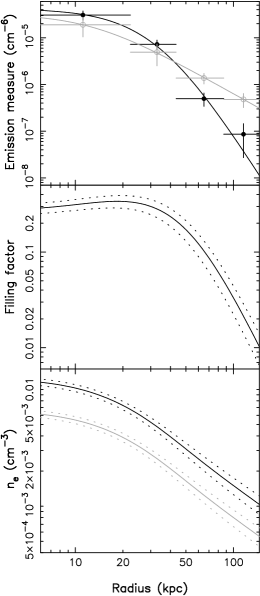
Figure 6: Upper panel: Emission-measure profiles of the hot (open circles) and cool (filled circles) components. Black and gray lines are the best-fit $\beta$ models. Middle panel: Filling factor profile of the cool component and the $1\sigma$ errors (dotted lines). Lower panel: electron density profiles of the hot (gray) and cool (black) components and the $1\sigma$ errors (dotted lines).

4.1 Single-phase gas profile

The single-phase gas density profile can be easily obtained from the observed surface brightness profile. We extract the surface brightness profiles in the 0.5–3.0 keV energy band for both source and blank sky data sets. The vignetting correction and background subtraction are performed using the same method as described in § 2. Since the cooling function, $\Lambda$, depends significantly on the temperature and metal abundance in the temperature range found in groups and cool clusters (see Figure 5), we need to take the $\Lambda$ profile into account when deriving the gas density profile from the observed surface brightness (Pratt & Arnaud 2003). We calculate the $\Lambda$ profile by using an absorbed VAPEC model that is convolved with the instrumental response in XSPEC. The parameters in the VAPEC model are fixed at the best-fit projected temperature and abundance profiles, which have been given in § 3.2.3 and § 3.2.1. From the center to the outmost region, the cooling function decreases with radius by $40\%$. Diving the observed surface brightness by the $\Lambda$ profile gives rise to the projected emission measure, which is proportional to $\int n^{2}_{\rm e}{\mathrm{d}}\ell$. Since the resultant projected emission measure profiles of MOS1, MOS2 and pn are well consistent with each other, we only display the averaged result in Figure 5.

We fit the projected emission measure profile with the standard $\beta$ model (Cavaliere & Fusco-Femiano 1976). If no correction of the XMM PSF is made, the projected emission measure profile is well modeled by a single $\beta$ model with $\beta=0.419\pm 0.001$, $r_{\rm c}=0.195\pm 0.001\arcmin$, and $EM_{0}=1.15\pm 0.01\times 10^{-3}$ cm^-5 ($\chi_{\nu}^{2}=142.1/82$). When the convolution of the XMM PSF is performed, we find that the fit is equally good, with $\beta=0.415\pm 0.001$, $r_{\rm c}=0.105\pm 0.001\arcmin$, and $EM_{0}=2.68\pm 0.01\times 10^{-3}$ cm^-5 ($\chi_{\nu}^{2}=142.9/82$). Both values of $\beta$ agree nicely with the power-law relation of $\beta=(0.44\pm 0.06)T^{0.20\pm 0.03}$ found by Sanderson et al. (2003). Note that the relatively large $\chi_{\nu}^{2}$ is caused by the anomalous fluctuations of the surface brightness profile, which can not be reduced even if the projected emission measure profile is fitted with a two-component model.

Finally, we deproject the $\beta$ model (PSF corrected) by using the inverse Abell integral to calculate the gas density profile (e.g. Sarazin 1986). The resulting electron density profile is plotted in Figure 5 with the central electron density $n_{\rm e0}=3.27\pm 0.01\times 10^{-2}$ cm^-3. The $n_{\rm e0}$ is calculated from the best-fit parameters of the $\beta$ model using the Monte Carlo method: We first generate $10^{5}$ random distributions of the parameters ($EM_{0}$, $r_{\rm c}$ and $\beta$) around the best-fit values with the standard deviations found above, using a normal probability distribution. We then compute $n_{\rm e0}$ for each set of the random ($EM_{0}$, $r_{\rm c}$ and $\beta$). Finally, we obtain the mean of the $10^{5}$ $n_{\rm e0}$ and its standard deviation. Throughout this paper, we use this method to calculate the quantities and their errors, such as the filling factor and electron densities in § 4.2, the gas entropy, cooling time and masses in § 5, the SN type fractions and mass-to-light ratios in § 6.2, in which the measurement errors of all the related parameters are taken into account.

We have also tried to obtain the gas density profile from the normalization parameter, $K\propto n^{2}_{\rm e}V$, which is obtained in the deprojected spectral fittings with the 1T model in § 3.2.3. The derived electron density is in good agreement with that obtained from the surface brightness profiles, except for the central region where the former is smaller than the latter by $\sim 43\%$. This again illustrates the defect of the 1T model.

4.2 Two-phase gas profile

In this section, we use the best-fit normalization parameters obtained in the deprojected 2T spectral fittings to calculate the gas density distributions for the multiphase gas in the inner part of the group. We reproduce four deprojected spectra within $2.4\arcmin$, and fit them with a two temperature VAPEC model. We fix metal abundances to the abundance profiles found in § 3.2.2 and assume that the temperatures of the hot and cool phases are spatially constant at the best-fit deprojected values of 1.56 keV and 0.83 keV, respectively. The emission measure of each phase is straightforwardly calculated using the normalization parameters in the VAPEC model and is then modeled with a single $\beta$ model (see Figure 6),

$$EM(R)=EM_{0}\left[1+\left(\frac{R}{R_{\rm c}}\right)^{2}\right]^{-3\beta},$$ (2)

where $R$ is the 3-dimensional radius.

Similarly to Ikebe et al. (1999), we define the volume-filling factor of the cool component $f(R)$ as $EM_{\rm c}(R)=n^{2}_{\rm g,c}(R)f(R)$, where $n_{\rm g,c}$ is the gas number density of the cool component. Thus, the emission measure of the hot component can be expressed as $EM_{\rm h}(R)=n^{2}_{\rm g,h}(R)[1-f(R)]$, where $n_{\rm g,h}$ is the gas number density of the hot component. Assuming local pressure balance between the two phases, $n_{\rm g,c}(R)T_{\rm c}=n_{\rm g,h}(R)T_{\rm h}$, we are able to calculate the filling factor and subsequent radial gas density distributions of the hot and cool components. As shown in Figure 6, $f(R)$ becomes smaller than $\sim 0.1$ outside $\sim 60$ kpc ($1\arcmin$), indicating that the cool gas occupies only a small fraction of the volume therein.

5 Gas entropy, cooling time and mass distributions

We will derive other dynamical quantities of the IGM such as gas entropy, cooling time, gas mass and total mass, as well as gas mass fraction, using the deprojected temperature profile shown in Figure 4 and the radial distribution of the gas density given in § 4.1 and § 4.2.

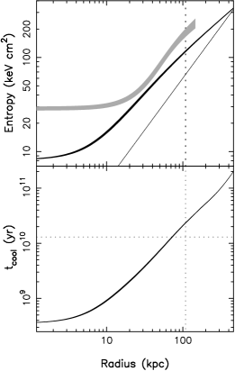
Figure 7: Gas entropy (upper) and cooling time (lower) profiles with $1\sigma$ errors for the single-phase gas (black region) and two-phase gas (gray region). The solid line represents $S(r)\propto r^{1.1}$, predicted by purely shock heating (Tozzi & Norman 2001). The vertical dotted line marks $0.1r_{200}$, and the horizontal line marks the Hubble time.

Figure 8: Radial profiles of gas mass, total mass and gas mass fraction of the single-phase (black) and two-phase (gray) gas with $1\sigma$ errors. Dotted lines represent the results obtained by assuming the gas is spatially isothermal.

Following the convention in the literature (e.g. Ponman, Cannon & Navarror 1999), for the single-phase gas we define the gas entropy as $S=k_{\rm B}T/n_{\rm e}^{2/3}$, and the cooling time as $t_{\rm cool}=\frac{5}{2}\frac{n_{\rm g}k_{\rm B}T}{n_{\rm e}n_{\rm H}\Lambda}$. It turns out that the resulting gas entropy increases monotonically with radius, and does not show an isentropic floor at the central region as far as can be resolved with the XMM instruments (Figure 7). The gas cooling time appears to be shorter than the Hubble time within $\sim 80$ kpc, where the gas has been found to have a multiphase nature (§ 3.3). For the two-phase gas, we calculate the entropy as

$$S=\exp\left[\frac{fn_{\rm e,c}\ln S_{\rm c}+(1-f)n_{\rm e,h}\ln S_{\rm h}}{fn_{\rm e,c}+(1-f)n_{\rm e,h}}\right],$$ (3)

where the $S_{\rm c}$ and $S_{\rm h}$ are the gas entropies of the cool and hot components, respectively. As seen in Figure 7, the derived entropy of the two-phase gas is larger than that of the single-phase gas by a factor of $\sim 3$ at the center and of 1.3–2 for $R>$20 kpc.

If the IGM is single-phase, we calculate the gas mass by integrating the gas density over the group volume as $\int\mu m_{\rm p}n_{\rm g}{\mathrm{d}}V$. If the IGM is two-phase, we calculate the gas mass of the cool and hot component using $\int\mu m_{\rm p}n_{\rm g,c}f{\mathrm{d}}V$ and $\int\mu m_{\rm p}n_{\rm g,h}(1-f){\mathrm{d}}V$, respectively, where $\mu=0.6$ is the mean molecular weight, and $m_{\rm p}$ is the photon mass.

The total gravitational mass distribtuion is derived under the assumption of hydrostatic equilibrium:

$$M(<R)=-\frac{R^{2}}{\rho_{\rm g}G}\frac{dP}{dR},$$ (4)

where, $P$ is the gas pressure that is expressed as $P=n_{\rm g}k_{\rm B}T$ for a single-phase gas, or $P=n_{\rm g,c}k_{\rm B}T=n_{\rm g,h}k_{\rm B}T$ for a two-phase gas. $\rho_{\rm g}$ is the gas mass density, defined as $\rho_{\rm g}=\mu m_{\rm p}n_{\rm g}$ for a single-phase gas and as $\rho_{\rm g}=\mu m_{\rm p}[fn_{\rm g,c}+(1-f)n_{\rm g,h}]$ for a two-phase gas.

In Figure 8, we display the spatial distributions of the gas mass and total gravitating mass, as well as the distribution of the gas mass fraction. In 30–80 kpc, the gas mass, total mass and gas mass fraction obtained under the two-phase assumption are consistent with those given by assuming that the gas is single-phase. In the inner regions, however, the masses derived from the two-phase assumption are 3–5 times lower than those obtained with the single-phase assumption. This can be attributed to the enhanced emission of the cool component in the 2T model. Using the single-phase assumption, we find that the gas mass fraction rises rapidly with radius to $\sim 0.15h^{-3/2}_{50}$ at $R\sim 462h^{-1}_{50}$ kpc.

We have also examined the effect of the temperature gradient on the determination of total mass. We find that the isothermal assumption leads to an overestimation of the total mass by $17\%$–$30\%$ within 80 kpc, where the gradient in temperature profile appears to be positive. In 80–430 kpc, where the temperature demonstrates a negative gradient, the isothermal assumption can result in an underestimation of the total mass by $48\%$ at most. If the observed data are further extrapolated outside 430 kpc, the isothermal assumption results in an overprediction of the total mass again. At $R\sim 800h^{-1}_{50}$ kpc, the typical value of the virial radius of galaxy group at 1 keV, the overestimation is about $17\%$.

We have investigated the mass distribution models that are suggested by high resolution N-body simulations, such as the generalized NFW models (GNFW), $\rho(r)=\frac{\rho_{\rm s}}{(r/r_{\rm s})^{\alpha}(1+r/r_{\rm s})^{3-\alpha}}$. The two free parameters $\rho_{\rm s}$ and $r_{\rm s}$ are determined by fitting the observed deprojected temperature profile with that predicted by assuming that the gas (described as $\beta$ model in § 4.1) is in hydrostatic equilibrium with the underlying dark matter-dominated gravitational potential well. Unfortunately, we fail to find an acceptable fit with any possible GNFW models by setting $\alpha=1$ (Navarro, Frenk & White 1997, NFW), or $\alpha=1.5$ (Moore et al. 1999), or $\alpha=2$. On one hand, we have only 6 data points which may be insufficient to give a stringent constraint on the models. On the other hand, the temperature distribution of this group is complex, for example, the existence of two-phase components at the central region, so the employment of a single-temperature assumption is over-simple.

6 Discussion

6.1 Gas temperature profile

Extrapolating the observed temperature and density profiles to large radii, we can estimate the virial radius of the group, $r_{200}$, the radius within which the mean mass overdensity is 200 times the critical density of the universe. This yields $r_{200}=786h^{-1}_{50}$ kpc. Such a value is, nevertheless, $27\%$ smaller than the one ($r_{200}=1083h^{-1}_{50}$ kpc) derived from the empirical relation $r_{200}=1.138(T/{\rm keV})^{1/2}(1+z)^{-3/2}h^{-1}_{50}$ Mpc found from the numerical simulations (Navarro, Frenk & White 1995). Regardless of the fact that this empirical relation may significantly overpredict $r_{200}$ in small halos (Sanderson et al. 2003), we will adopt $r_{200}=1083h^{-1}_{50}$ kpc below, unless stated otherwise, for the convenience of comparing with other studies. In this case, the observed diffuse X-ray emission of the group extends to $\sim 45\%$ of the virial radius.

The temperature profile of RGH 80 follows more or less a universal form as has already been found in some groups of galaxies observed with $\it ROSAT$ (Mulchaey 2000, and references therein) and $\it ASCA$ (Finoguenov et al. 2002a): Gas temperature is at its minimum ($0.83$ keV) at the center, rises to the maximum value at a small radius ($0.11r_{200}$), and then drops gradually with radius. Similar temperature profiles have been found recently with XMM-Newton and $\it Chandra$ in galaxy groups NGC 1550, NGC 2563, NGC 5044, and MKW 4 (Sun et al. 2003; Mushotzky et al. 2003; Buote et al. 2003a; O’Sullivan et al. 2003). Yet, we note that there are still some groups in which a flat temperature profile at large radii is reported, such as NGC 1399, NGC 2300, NGC 4325 and AWM 4 (Boute 2002; Mushotzky et al. 2003; O’Sullivan & Vrtilek 2003; see Sun et al. 2003 for a comprehensive summary).

6.2 Gas metallicity and supernovae enrichment

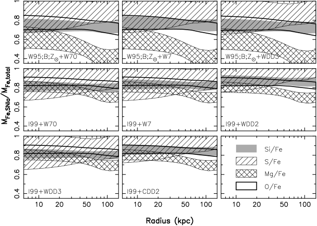
Figure 9: The radial profiles of SN type fractions derived from the observed abundance ratio pattern. Only the results of those models in which consistent SN type fractions can be achieved with the observed Si/Fe, S/Fe, O/Fe and Mg/Fe ratios are shown.

With the abundance ratios derived in § 3.2.1 and § 3.2.2, we are able to probe the origin of the heavy elements in RGH 80 and to distinguish between the different contributions of type Ia and type II supernovae. Following Gibson, Loewenstein & Mushotzky (1997; see also Ishimaru & Arimoto 1997), we take $M_{\rm Fe,SNIa}/M_{\rm Fe,total}$ to quantify the roles played by SN Ia in contributing to the metal abundances. The relative frequency of SN Ia to the total SNe, $\zeta$, can be determined by the ratio of the total mass of the $\alpha$ elements to the total iron mass, together with the SN models.

For SN Ia, we adopt seven updated models listed in table 3 of Iwamoto et al. (1999), namely, the W70 model in which the initial metallicity is assumed to be zero, the W7 model and five delayed detonation models, WDD1–3 and CDD1–2. We also utilize the SN II model listed in the same table (the I99 model hereafter), which is similar to the T95 model in Gibson et al. (1997; see also Tsujimoto et al. 1995). In addition, we also choose the four representative “W95” models for SN II (W95;A;$10^{-4}$Z_⊙, W95;A;Z_⊙, W95;B;$10^{-4}$Z_⊙, W95;B;Z_⊙; Gibson et al. 1997; Woosley & Weaver 1995). For all the SN II models, the elemental yields are integrated over 10 M_⊙ to 50 M_⊙ by using the Salpeter IMF.

We first utilize the metal abundances obtained from the spectral fittings with the projected 2T model, in which the abundances are better constrained than those with the 1T model at the central region. Based on the best-measured Si/Fe ratio, we find that $90\%$–$100\%$ of the iron mass was produced by SN Ia according to the SN Ia model WDD1/CDD1 together with any of the SN II models. The fraction decreases to $70\%$–$90\%$ if the other combined SN models are used. The SN Ia fractions estimated with the observed O/Fe ratio agree well with those obtained with the Si/Fe ratio. The fractions range from $65\%$ to $90\%$ for any combinations of the SN models.

The S/Fe ratio, on the other hand, gives a somewhat loose constraint on the SN Ia contribution, which ranges from $65\%$ to $100\%$ for any possible combinations except for those combined with WDD1 and CDD1. These two SNIa models (WDD1 and CDD1) seem to overproduce S relatively to Fe, which results in a unreasonably high SN Ia fraction ($>1$). With the observed Mg/Fe ratio and the I99 model, we obtain a consistent SN Ia fraction with that derived from the O/Fe, S/Fe and Si/Fe ratios. However, if the four W95 models are in use, we tend to underestimate the Mg yields, which leads to a relatively low SN Ia fraction.

Finally, we find that in those combined models where the SN Ia model is not WDD1 or CDD1, consistent SN type fractions can be achieved with the observed abundance ratios of Si/Fe, S/Fe and O/Fe. If the model combination is I99+W70, I99+W7, I99+WDD2, I99+WDD3, or I99+CDD2, consistent SN Ia fractions can be obtained with the abundance ratios of Si/Fe, S/Fe, O/Fe and Mg/Fe. If the model combination is W95;B;Z_⊙+W70, W95;B;Z_⊙+W7, or W95;B;Z_⊙+WDD3, a marginally consistent SN Ia fraction can be obtained in $R<20$ kpc with the above four abundance ratios (see Figure 9).

Table 3: The IGM metal mass to light ratios

Radius	$M_{\rm gas}$	$L_{\rm B}$	$M_{\rm Fe}/L_{\rm B}$	$M_{\rm O}/L_{\rm B}$	$M_{\rm Mg}/L_{\rm B}$	$M_{\rm Si}/L_{\rm B}$	$M_{\rm S}/L_{\rm B}$
(kpc)	($10^{12}M_{\odot}$)	$(10^{11}L_{\odot})$	$(10^{-3}M_{\odot}/L_{\odot})$	$(10^{-2}M_{\odot}/L_{\odot})$	$(10^{-3}M_{\odot}/L_{\odot})$	$(10^{-3}M_{\odot}/L_{\odot})$	$(10^{-4}M_{\odot}/L_{\odot})$
462	$3.10\pm 0.01$	2.89	$3.75\pm 0.24$	$1.19\pm 0.75$	$1.22\pm 0.45$	$1.94\pm 0.50$	$9.20\pm 5.33$
786	$7.88\pm 0.03$	4.39	$4.67\pm 0.38$	$1.91\pm 1.56$	$1.10\pm 0.66$	$3.00\pm 1.03$	$13.95\pm 11.01$

In terms of the radial behaviors of the SN Ia fractions derived from the abundance ratios shown in Figure 9, it appears that the SN Ia fraction remains almost constant with radius at $\sim 85\%$ for the SNII model I99 or at $\sim 72\%$ for the SNII model W95;B;Z_⊙. It is likely that the decline in the SN Ia fraction with increasing radius derived from the Mg/Fe ratio is an artifact because Mg lines are blended with the outskirt of the Fe L-shell complex, and therefore are measured less accurately than O and Si. The resulting SN type fraction agrees with those obtained from previous $\it ASCA$ observation of galaxy groups (Finoguenov & Ponman 1999) and from recent XMM-Newton and $\it Chandra$ observations of NGC 5044 (Buote et al. 2003b), NGC 1399 (Buote 2002) and NGC 1550 (Sun et al. 2003).

We then employ the abundance ratios obtained in the projected 1T model fittings to examine the SN models and contributions to the iron mass of different types of SNe. We find that only in models I99+WDD1 and I99+CDD1 can a marginally consistent SN Ia fraction of $\sim 80\%$ be derived from the observed abundance ratios of Si/Fe, S/Fe, O/Fe and Mg/Fe.

We can calculated the ratios of the metal mass in the IGM to the total blue luminosity of the galaxies in the group for the measured elements within the observed region of $462h^{-1}_{50}$ kpc using the elemental abundances obtained from the projected 1T model fittings. The metal mass of element $i$ is calculated by

$$M_{i}(<R)=\int_{0}^{R}4\pi m_{i}Z_{\odot,i}Z_{i}(r)n_{\rm H}(r)r^{2}{\mathrm{d}}r,$$ (5)

where $m_{i}$ is the atomic mass of element $i$. For the total blue luminosity, we take the magnitudes $m_{\rm zwi}$ in the Zwicky B(0) system from Ramella et al. 1995, and convert them to magnitude B with the relation $m_{\rm zwi}=B+0.35$ given by Gaztanaga & Dalton (2000). The metal mass-to-light ratios within the virial radius of $786h^{-1}_{50}$ kpc are also derived by extrapolating the gas distribution to $r_{200}$ and assuming that the abundances beyond the observed region are the same as those in the outmost shell. We summarize the results in Table 3.

It turns out that the derived Fe $M/L$ is $\sim 2$ times lower than the corresponding typical value of clusters (Arnaud et al. 1992; Loewenstein & Mushotzky 1996; Renzini 1997; Finoguenov et al. 2001). Moreover, Si $M/L$ between clusters and this group differs by a factor of $\sim$ 10. This is consistent with the findings of Finoguenov et al. (2001). The lower values of metal mass-to-light ratios of the group may imply that the group has lost some of the enriched gas that was produced by the galaxies in the group.

6.3 Entropy

The observed gas entropy of RGH 80 at $0.1r_{200}$ is $\sim 90h^{-1/3}_{50}$ keV cm² for a single-phase gas model, which seems to be a typical value for groups of $\sim 1$ keV (Lloyd-Davis et al. 2000; Ponman, Sanderson & Finoguenov 2003). The entropy reaches $\sim 185h^{-1/3}_{50}$ keV cm² if gas is assumed to be two-phase. Additionally, gas entropy increases with radius as $r^{0.81}$ in the region of $r>0.01r_{\rm vir}$ and as $r^{1.0}$ in the region of 30 kpc$<r<$ 100 kpc for the single-phase and two-phase assumptions, respectively. As a result, the derived radial entropy profiles from the single-temperature assumption are flatter than that expected from purely shock heating ($S(r)\propto r^{1.1}$; Tozzi & Norman 2001) throughout the whole group. This implies that the IGM may have suffered from non-gravitational effects such as radiative cooling, heating by supernovae and/or AGNs, even at large radii. The preheating scenario, in which gas is pre-heated and subsequently collapses adiabaticly, predicts an isentropic core of 50–100 keV cm² within $0.1r_{\rm vir}$ for groups of $2\times 10^{13}$ M_⊙ in order to reconcile the theoretically expected $L_{\rm X}$–$T$ relation with observation (Tozzi & Norman 2001). However, the entropy of RGH 80 we obtained starts to increase rapidly from an inner radius of as small as 0.01–0.02$r_{\rm vir}$, which disagrees with the prediction of preheating model.

The expected entropy profile based on radiative cooling model or internal heating model, or cooling plus internal heating model (Finoguenov et al. 2002b; Borgani et al. 2002; Brighenti & Mathews 2001) resembles the observed data of this group in shape. In particular, it has already been found that the cooling may marginally reproduce the observed scaling relations of $S(0.1r_{\rm vir})$–$T$ (Voit & Bryan 2001) and $L_{\rm X}$–$T$ (Muanwong et al. 2002; Wu & Xue 2002a), and may even be responsible for the scale-dependence of the IGM mass function (Wu & Xue 2002b). However, the cooling process suffers from the so-called cooling crisis (Balogh et al. 2001), and is also inefficient in the explanation of the observed X-ray properties of groups and clusters (Bower et al. 2001). Inclusion of a suitable energy feedback from galaxy formation has been suggested to prevent the IGM from overcooling and supply the IGM with additional energy (Borgani et al. 2002). Indeed, Xue & Wu (2003) pointed out that a combination of cooling and heating can explain simultaneously the observed global X-ray properties of groups and clusters (e.g. gas entropy distribution and $L_{\rm X}$–$T$ relation), and the observational limits on the contribution of the diffuse IGM in virialized halos to the X-ray background within the framework of standard CDM structure formation with an amplitude of matter power spectrum $\sigma_{8}\approx 0.7$. Therefore, our observation seems to favour the heating plus cooling model.

6.4 comparison with scaling relations

We now compare the total mass and gas fraction of RGH 80 with the expectations from the scaling relations of $f_{\rm gas}$–$T$ and $M$–$T$ derived by Sanderson et al. (2003), adopting a virial radius of $786h^{-1}_{50}$ kpc. The gas fractions at $0.3r_{200}$ and $r_{200}$ are $0.06h^{-3/2}_{50}$ and $0.25h^{-3/2}_{50}$, respectively, which are comparable to the upper limits of group gas fractions of in the Sanderson et al. (2003) sample. This indicates that RGH 80 is a relatively gas rich system. The total masses of the group ($1.53\times 10^{13}h^{-1}_{50}M_{\odot}$ within $0.3r_{200}$ and $3.14\times 10^{13}h^{-1}_{50}M_{\odot}$ within $r_{200}$) agree nicely with what are expected from the observed $M(0.3r_{200})$–$T$ and $M(r_{200})$–$T$ relations of groups and clusters (Sanderson et al. 2003), respectively.

The velocity dispersion and bolometric X-ray luminosity of RGH 80 are $450$ km s^-1 (Ramella et al. 2002) and $2.06\times 10^{43}h^{-2}_{50}$ erg s^-1 within $462h^{-1}_{50}$ kpc, respectively. These values are comparable to the expectations from the observed $L_{\rm X}$–$\sigma$ relation for groups and clusters (Wu, Xue & Fang 1999), though the group appears to be relatively luminous in the $L_{\rm X}$–$T$ plane (Xue & Wu 2000).

7 Conclusions

We summarize below the main conclusions from our analyses of the XMM-Newton observations of the galaxy group of RGH 80.

• The X-ray emission of the group is detected out to $\sim 7.67\arcmin$, or $462h^{-1}_{50}$ kpc, corresponding to $0.45r_{200}$. The group seems to be relatively gas rich and luminous with respect to its temperature ($1.01\pm 0.01$ keV).

• Spectral analysis shows that the temperature profile, which increases from the center and then declines with radius after reaching a plateau around $0.11r_{200}$, follows a universal profile (Mulchaey 2000) and that the abundance profile of each measured element decreases monotonically with radius.

• In the central region, the X-ray emission of the gas is better modeled by a two-temperature spectral model, with temperatures of 0.82 and 1.51 keV and the Galactic absorption, than by a single temperature or cooling flow models. Beyond $\sim 60$ kpc ($1\arcmin$), the volume filling factor of the cool component, $f(R)$, becomes smaller than $\sim 0.1$, indicating that the cool gas occupies only a small fraction of the volume therein.

• The gas entropy distribution derived from single-temperature assumption deviates from the prediction of the over the whole observed region, The isentropic core at the center expected from preheating model does not show up. Nevertheless, our derived entropy profile resembles what is predicted by radiative cooling model or internal heating model or cooling plus heating model.

• Both the abundance ratios of Fe/O and Fe/Si are very high showing a large SN Ia dominance, which is higher than that for M87 (Matsushita et al. 2004) and comparable to or slightly higher than that for Centaurus cluster (Matsushita et al. 2004). With the abundance ratio pattern of the hot gas, we estimate that $\sim 85\%$ (I99) or $\sim 72\%$ (W95;B;Z_⊙) of the iron mass is contributed by SN Ia. This SN type fraction remains almost constant against radius. We find that S is significantly overproduced by the two delayed detonation models WDD1 and CDD1, while Mg is slightly underproduced by the four W95 models considered here.

- (1) Anders, E., & Grevesse, N. 1989, GeCoA, 53, 197
- (2) Arnaud K.A., 1996 Astronomical Data Analysis Software and Systems V, eds. Jacoby G. and Barnes J., p17, ASP Conf. Series volume 101
- (3) Arnaud, M., Rothenflug, R., Boulade, O., Vigroux, L., & Vangioni-Flan, E. 1992, A&A, 254, 49
- (4) Arnaud, M., Neumann, D., Aghanim, N. et al. 2001, A&A, 365, L80
- (5) Arnaud, M., Majerowicz, S., Lumb, D., et al. 2002, A&A, 390, 27
- (6) Balogh, M., Pearce, F.R., Bower, R.G., & Kay, S.T. 2001, MNRAS, 326, 1228
- (7) Böhringer, H., Matsushita, K., Churazov, E., Ikebe, Y., & Chen, Y. 2002, A&A, 382, 804
- (8) Borgani, S., Governato, F., Wadsley,J. et al. 2002, ApJ, 336, 409
- (9) Bower, R.G., Benson, A.J., Lacey, C.G., et al. 2001, MNRAS, 325, 497
- (10) Brighenti, F., & Mathews, W.G. 2001, ApJ, 2001, 553, 103
- (11) Buote, D.A. 2000, MNRAS, 311, 176
- (12) Buote, D.A. 2002, ApJ, 574, L135
- (13) Buote, D.A., Lewis, A.D., Brighenti, F., & Mathews, W.G. 2003a, ApJ, 594, 741
- (14) Buote, D.A., Lewis, A.D., Brighenti, F., & Mathews, W.G. 2003b, ApJ, 595, 151
- (15) Cavaliere, A., & Fusco-Femiano, R. 1976, A&A, 49, 137
- (16) David, L.P., Slyz, A., Jones, C., Forman, W., & Vrtilek, S.D. 1993, ApJ, 412, 479
- (17) Davis, D.S., Mulchaey, J.S., & Mushotzky, R.F. 1999, ApJ, 511, 34
- (18) Dickey, J.M., & Lockman, F.J. 1990, ARA&A, 28, 215
- (19) Edge, A.C., & Stewart, G. 1991, MNRAS, 252, 414
- (20) Finoguenov, A., & Ponman, T.J 1999, MNRAS, 305, 325
- (21) Finoguenov, A., Arnaud, M., & David, L.P 2001, ApJ, 555, 191
- (22) Finoguenov, A., Jones, C., Böhringer, H., & Ponman, T.J 2002a, ApJ, 578, 74
- (23) Finoguenov, A., S. Borgani, L. Tornatore, Böhringer, H., & Ponman, T.J 2002b, ApJ, 578, 74
- (24) Freyberg, M.J., Pfeffermann, E., & Briel U.G. 2001, New Visions of the X-ray Universe in the XMM-Newton and Chandra Era, 26–30, November 2001, ESTEC, The Netherlands
- (25) Gaztanaga, E., & Dalton, G.B. 2000, MNRAS, 312, 417
- (26) Gibson, B.K., Loewenstein, M., & Mushotzky, R.F. 1997, ApJ, 290, 623
- (27) Helsdon, S., & Ponman, T.J. 2000, MNRAS, 315, 356
- (28) Ikebe, Y., Makishima, K., Fukazawa, Y., et al. 1999, ApJ, 525, 58
- (29) Ikebe, Y. 2001, Tracing Cosmic Evolution with Clusters of Galaxies, Sesto Pusteria, Bolzano, Italy, July 3-6, 2001, astro-ph/0112132
- (30) Ishimaru Y., & Arimoto, N. 1997, PASJ, 49, 1
- (31) Iwamoto, K., Brachwitz, F., Nomoto, K., et al. 1999, ApJS, 125, 439
- (32) Kaastra, J.S., Ferrigno, C., Tamura, T., et al. 2001, A&A, 365, 99
- (33) Katayama, H., Takahashi, I., Ikebe, Y., Matsushita, K., & Freyberg, M.J. 2002, astro-ph/0210135
- (34) Lloyd-Davies, E.J., Ponman, T.J., & Cannon, D.B. 2000, MNRAS, 315, 689
- (35) Loewenstein, M., & Mushotzky, R.F. 1996, ApJ, 466, 695
- (36) Lumb, D. 2002, XMM-SOC-CAL-TN-0016
- (37) Lumb, D., Warwick, R.S., Page, M., & De Luca, A 2002, A&A, 389, 93
- (38) Mahdavi, A., Böhringer, H., Geller, M.J., & Ramella, M. 2000, ApJ, 534, 114
- (39) Majerowicz, M., Neumann, D.M., & Reiprich, T.H. 2002, A&A, 394, 77
- (40) Matsushita, K.,Belsole, E., Finoguenov, A., & Böhringer, H. 2002, A&A, 386, 77
- (41) Matsushita, K., Finoguenov, A., & Böhringer, H. 2003, A&A, 401, 443
- (42) Matsushita, K., Böhringer, H., Takahashi, I., & Ikebe, Y. 2004, in preparation
- (43) Molendi, S. & Pazzolato, F. 2001, ApJ, 560, 194
- (44) Muanwong, O., Thomas, P.A., Kay, S.T., Pearce, F.R. 2002, MNRAS, 336, 572
- (45) Mulchaey, J.S. 2000, ARA&A, 38, 289
- (46) Mushotzky, R., Figueroa-Feliciano, E., Loewenstein, M., & Snowden S.L. 2003, astro-ph/0302267
- (47) Navarro, J.F., Frenk, C.S., & White, S.D.M. 1995, MNRAS, 275, 720
- (48) O’Sullivan, E., Vrtilek, J.M., Read, A.M., David, L.P., & Ponman, T.J. 2003, astro-ph/0308255
- (49) O’Sullivan, E., & Vrtilek, J.M. 2003, astro-ph/0310099
- (50) Peterson, J.R., Paerels, F.B.S, Kaastra, J.S., et al. 2001, A&A, 365, L104
- (51) Ponman, T.J., Cannon, D.B., & Navarro, J.F. 1999, Nature, 397, 135
- (52) Ponman, T.J., Sanderson, A.J.R., & Finoguenov, A. 2003, MNRAS, 343, 331
- (53) Pratt, G.W., Arnaud, M., & Aghanim, N. 2001, Proc. XXXVI Rencontres de Moriond: Galaxy Clusters and the High-Redshift Universe, eds. D.M. Neumann, F. Durret and J. Trân Thanh Van: astro-ph/0105431.
- (54) Pratt, G.W., & Arnaud, M. 2003, A&A, 408, 1
- (55) Ramella, M., Geller, M.J., & Huchra, J.P. 1989, ApJ, 344, 57
- (56) Ramella, M., Geller, M.J., Huchra, J.P., & Thorstensen, J.R. 1995, AJ, 109, 1458
- (57) Ramella, M., Geller, M.J., Pisani, A., & Da Costa, L.N. 2002, AJ, 123, 2976
- (58) Read, A.M., & Ponman, T.J. 2003, A&A, 409, 395
- (59) Renzini, A. 1997, ApJ, 488, 35
- (60) Sakelliou, I., Peterson, J.R., Tamura, T., et al. 2002, A&A, 391, 903
- (61) Sanderson, A.J.R., Ponman, T.J., Finoguenov, A., Lloyd-Davies, E.J., & Markevitch, M. 2003, MNRAS, 340, 989
- (62) Sarazin, C., 1986, Rev. Mod. Phys., 58, 1
- (63) Smith, R.K., Brickhouse, N.S., Liedahl, D.A., Raymond, J.C. 2001, ApJ, 556, L91
- (64) Sun, M., Forman, W., Vikhlinin, A., Hornstrup, A., Jones, C., & Murray, S.S. 2003, astro-ph/0308037
- (65) Tamura, T., Kaastra, J.S., & Peterson, J.R., et al. , 2001, A&A, 365, L87
- (66) Tozzi, P., & Norman, C., 2001, ApJ, 546, 63
- (67) Tsujimoto, T., Nomoto, K., Yoshii, Y., Hashimoto, M., Yanagida, S., & Thielemann, F.K. 1995, MNRAS, 277, 945
- (68) Voit, G.M., & Bryan, G.L. 2001, Nature, 414, 425
- (69) Voit, G.M., Bryan, G.L., Balogh, M.L., & Bower, R.G. 2002, ApJ, 576, 601
- (70) Voit, G.M., Balogh, M.L., Bower, R.G., Lacey, C.G., & Bryan, G.L., 2003, ApJ, 593, 272
- (71) Woosley S.E., & Weaver T.A. 1995, ApJS, 101, 181
- (72) Wu, X.P., Xue, Y.J., & Fang L.Z. 1999, ApJ, 524, 22
- (73) Wu, X.P., & Xue, Y.J. 2002a, ApJ, 569, 112
- (74) Wu, X.P., & Xue, Y.J. 2002b, ApJ, 572, L19
- (75) Xu, H., Kahn, S.M., Peterson, J.R., et al. 2002, ApJ, 579, 600
- (76) Xu, H., Jin, G., & Wu, X.P. 2001, ApJ, 553, 78
- (77) Xue, Y.J. & Wu, X.P., 2000, ApJ, 538, 65
- (78) Xue, Y.J. & Wu, X.P., 2003, ApJ, 584, 34