The 2dF Galaxy Redshift Survey: The blue galaxy fraction and implications for the Butcher-Oemler effect

Abstract

We derive the fraction of blue galaxies in a sample of clusters at $z<0.11$ and the general field at the same redshift. The value of the blue fraction is observed to depend on the luminosity limit adopted, cluster-centric radius and, more generally, local galaxy density, but it does not depend on cluster properties. Changes in the blue fraction are due to variations in the relative proportions of red and blue galaxies but the star formation rate for these two galaxy groups remains unchanged. Our results are most consistent with a model where the star formation rate declines rapidly and the blue galaxies tend to be dwarfs and do not favour mechanisms where the Butcher-Oemler effect is caused by processes specific to the cluster environment.

1 Introduction

The observation by Butcher & Oemler (1984) that clusters of galaxies contain a larger fraction of blue galaxies at progressively higher redshift (the Butcher-Oemler effect) contributed to the establishment of the current view of clusters as sites of active galaxy evolution, in which environmental influences dramatically alter the morphologies and star formation histories of their members.

However, as the number of clusters observed has increased, it has become clear that the Butcher-Oemler effect is not solely or simply an evolutionary trend. The large scatter observed in the blue fractions for clusters in narrow redshift ranges (Smail et al., 1998; Margoniner & de Carvalho, 2000; Goto et al., 2003a) implies the existence of environmental effects, which may compete with, and possibly mimic, evolutionary trends, if the cluster samples evolve with redshift.

Studies of the original Butcher-Oemler sample lend support to this scenario: Newberry et al. (1988) measured the surface densities and velocity dispersions of seven Butcher-Oemler clusters and found that the high and low redshift sample differ. Andreon & Ettori (1999) show that the X-ray luminosity of high redshift Butcher-Oemler clusters is higher than that of low redshift clusters, although the X-ray luminosity function of clusters does not evolve to $z\sim 0.8$ (Holden et al., 2002), arguing that the high redshift sample does not represent the progenitors of modern-day clusters. Similarly, both Smail et al. (1998) and Fairley et al. (2002) find a low blue fraction in their samples of X-ray selected clusters.

The blue fraction has also been observed to depend on a number of other factors, such as: the luminosity limit used and the cluster centric distance (Ellingson et al., 2001; Goto et al., 2003a), richness (Margoniner et al., 2001), cluster concentration (Butcher & Oemler, 1984) and, possibly, the presence of substructure (Metevier et al., 2000). These findings point to the necessity of understanding environmental effects on the blue fraction in order to disentangle evolutionary trends from selection biases in studies of clusters at high redshift.

The aim of the present paper is to study how the fraction of blue galaxies varies as a function of cluster properties and in the field at the same redshift in the local universe, in order to analyse the effects of environment in isolation from the evolutionary trends that give rise to the Butcher-Oemler effect. Lewis et al. (2002) and Balogh et al. (2003) have recently discussed how the star formation rate, as measured from the H$\alpha$ equivalent width, varies with environment within the 2dFGRS sample. However, colours provide a measure of the average star formation histories over longer timescales than H$\alpha$ and may therefore better reflect the influence of environment on galaxy properties, especially if the mechanisms responsible for the Butcher-Oemler effect operate on longer time frames, as is the case for harassment (Moore et al., 1996), for instance.

The structure of this paper is as follows: in the next section we present our analysis; selection of clusters, cluster members and a comparison field sample, definition of the radial and luminosity limits used, $k$-corrections, colour-magnitude relations, density measurements and a discussion of how the blue fraction and its error are measured. The main results are detailed in §3. below and we discuss these in §4. Throughout this paper we adopt a cosmology with $\Omega_{M}=0.3$, $\Omega_{\Lambda}=0.7$. It is normal to define $h\equiv H_{0}/100\,{\rm km\ s^{-1}\ Mpc^{-1}}$: here we suppress the $h$ scaling, so that the full explicit meaning of Mpc in length units is $h^{-1}$ Mpc; for absolute magnitudes $M$ stands for $M+5\log_{10}h$.

2 Analysis

In this work, we analyse how the blue fraction of galaxies varies as a function of cluster properties and field density at $z<0.11$; our purpose is to provide a local reference for studies of galaxy colour evolution in high redshift clusters (the Butcher-Oemler effect). It is therefore useful to reproduce, in our analysis, some of the features of the original Butcher & Oemler (1984) study, as this is the basis for most current work on the evolution of stellar populations of cluster galaxies.

The original analysis of Butcher & Oemler (1984) defined blue galaxies as being (i) within a radius containing 30% of the cluster population; (ii) brighter than a no-evolution $k-$corrected $M_{V}=-20$ and (iii) bluer by 0.2 magnitudes in $B-V$ (no-evolution and $k-$corrected) than the colour-magnitude relation defined by the cluster early-type galaxies. Below we describe how we implemented these prescriptions for our dataset.

2.1 Cluster and member selection

The clusters analyzed here are those studied by De Propris et al. (2003a) in their paper on the composite galaxy luminosity function. This sample consists of 60 clusters at $z<0.11$ containing at least 40 spectroscopic members and with average 85% completeness. Although these clusters share, to some extent, the biases of the Abell, APM and EDCC catalogues from which they were originally drawn (see De Propris et al. 2002 for details), these 60 objects provide an at least approximately complete and volume limited ensemble of nearby clusters, spanning a large range of properties (such as richness and velocity dispersion) determined from the same data (De Propris et al., 2002).

Cluster membership was determined via a ‘double gapping’ method, as described in greater detail in De Propris et al. (2002): for each putative cluster centre and redshift, we first required that the likely cluster members be surrounded by 1000 km s^-1 gaps on either side of the redshift distribution; we next computed a first estimate for the mean $cz$ and velocity dispersion ($\sigma_{r}$) and ranked all galaxies in order of distance from the mean $cz$. If galaxies had a ‘gap’ in redshift space from their neighbour larger than our first estimate of $\sigma_{r}$ all galaxies with a faster or slower velocity were excluded. This procedure yields a sample of cluster members which is likely to be relatively uncontaminated by interlopers (i.e. field galaxies with appropriate redshift but not dynamically bound to the cluster).

2.2 Aperture and luminosity selection

We calculate $r_{30}$ (the original aperture used by Butcher & Oemler 1984) by using all cluster members within a 3 Mpc radius from the central galaxy. We then choose an aperture than includes 30% of these galaxies. It is observed that the value of $r_{30}$ varies depending on cluster dynamics and central concentration. For this reason it may be generally more appropriate to use apertures based on cluster dynamical properties, in order to insure that all galaxies considered share the same environment in all clusters. Ellingson et al. (2001) advocate using $r_{200}$, the radius at which the cluster is 200 times denser than the general field (Carlberg et al., 1997), or its multiples. This is defined as:

$$r_{200}={{\sqrt{3}\sigma_{r}}\over{10H(z)}}$$

where $H(z)$ represents the redshift-dependent Hubble constant. In the following, we will use both $r_{200}$ and $r_{200}/2$ for our analysis.

The original limit by Butcher & Oemler (1984) corresponds to approximately 1.8 magnitudes below the $M^{*}$ point. Here, we use a magnitude limit 1.5 magnitudes fainter relative to our computed $M^{*}$ and we also analyse the effects of using fainter limits. This allows us to study a more consistent sample of galaxies in all clusters.

2.3 $k$-corrections

$B_{\rm J}-R_{\rm F}$ colours for all 2dFGRS galaxies were derived using data from the SuperCosmos survey (Hambly et al., 2001). Given the colours and redshifts we derived a $k$-correction in the following way.

The kcorrect package (Blanton et al., 2003a) fits a combination of templates to galaxy colour data, and thus yields a consistent $k$-correction. Although only two bands are available for the 2dFGRS, this approach was validated by fitting the full DR1 $u$$g$$r$$i$$z$ data, then comparing with the result of fitting $gr$ only. The differences in K-correction are generally at the 0.01 mag. level.

The main problem with kcorrect is that the templates are unable to describe extremely red galaxies ($B_{J}-R_{F}=1.26$ corresponding to $g-r=0.87$), and so a consistent $k$-correction cannot be obtained. In such cases, we took an alternative approach, based on the models of Bruzual & Charlot (2003). Each galaxy was modelled by a single burst, varying the age until the observed colour was matched at the given redshift. This age is degenerate with metallicity; in practice, we assumed 0.4 times Solar metallicity ($Z=0.008$), except for very red galaxies where a current age of $>13$ Gyr was required. In these cases, the current age was set at $13$ Gyr and the metallicity increased until the colour was matched. For red galaxies, $k$-corrections deduced in this way agree almost exactly with the results of kcorrect, and we were able to match smoothly from one to the other to deal with the very red galaxies that kcorrect cannot model. The results differ for extremely blue galaxies (at the 0.1 mag. level), but a single burst is a rather unrealistic model in such cases and the results of kcorrect are to be preferred where they are consistent.

The fitting functions given below describe the $k$-correction results for all colours of practical interest at $z<0.3$, to within a maximum error of about 0.02 mag. Given the intrinsic uncertainties in both photometric modelling and calibration, and in the interests of clarity, these residuals were ignored and the fit was treated as exact.

 

$${k(B_{\rm J})=\,}$$

 

$$k(R_{\rm F})=(-0.08+1.45x)y-(2.88+0.48x)y^{2}$$

where

$$x=B_{\rm J}-R_{\rm F}$$

$$y=z/(1+z)$$

2.4 Colour-magnitude relations

For all clusters, we determine the colour-magnitude relation by carrying out a least absolute deviation regression fit to the observed colour distribution (Armstrong & Kung, 1978). The average observed slope is about $-0.019\pm 0.003$, consistent with the relation observed in the Coma galaxies for $V-R$ (Eisenhardt et al. 2004, in preparation). There appears to be some cluster-to-cluster variation in the slope, but this may be due to small number statistics in some cases.

We carry out the same analysis for field galaxies, but we divide the sample according to local density (see below for details). The slope for the field galaxies is $\sim-0.013\pm 0.001$. These slopes were calculated robustly and jackknife resampling was then used to compute the errors on the values of the slopes. The slopes of the relations for field and cluster galaxies appear to be different at about the $2\sigma$ level, but we do not regard this as compelling (cf., Hogg et al. 2004 for a similar study from Sloan colours).

The 2dFGRS SuperCosmos colours can be transformed to the SDSS $g$ and $r$ bands using the following equations:

$$B_{\rm J}=g+0.15+0.13(g-r)$$

$$R_{\rm F}=r-0.13$$

A difference in $B-V$ of 0.2 magnitudes from the ridge line defined by early-type galaxies is equivalent to a 0.2 magnitude difference in $g-r$ (Goto et al., 2003a). From the above equation we then derive that the corresponding difference in $B_{\rm J}-R_{\rm F}$ is 0.23 magnitudes. Fig. 1 shows the colour-magnitude relation and the colour distribution, marginalised over the derived colour magnitude relation, for a few representative clusters.

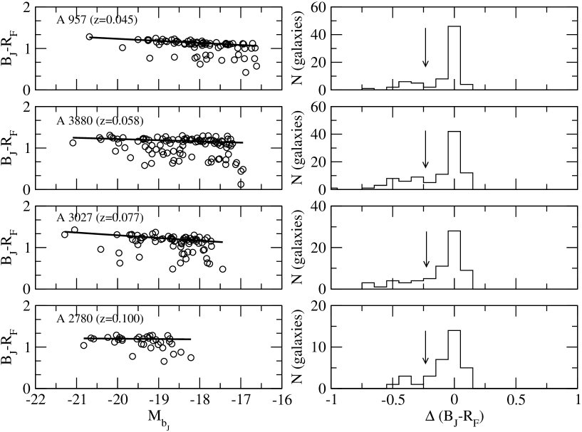
Figure 1: Colour-magnitude relation (left) and histogram (right) of marginalised colour distribution (opposite each colour-magnitude relation) for four representative clusters. The arrow in the histogram indicates the blue/red separation (see text)

2.5 Calculation of local density

For field galaxies, the only relevant ‘environmental’ property is their local density. We calculate this by computing the number of galaxies to $M_{B_{\rm J}}=-19$ in an 8 Mpc sphere centred on each galaxy, with appropriate completeness corrections. A detailed description of this procedure is given in Croton et al. (2004). Unfortunately, this assumes that all radial velocities are due to the smooth Hubble flow and can be used as proxies for distance. This is not applicable in the cluster environment, where the galaxies have turned around and no longer participate in the cosmological expansion (see, e.g., Cooperstock et al. 1998). For clusters, therefore, we assume that all members are effectively within $r_{200}$ and calculate the density in an 8 Mpc sphere containing only cluster members. This places the density for cluster galaxies on the same scale as that used for field galaxies. As we note below, this is likely to be a slight underestimate of the actual density (as some members may exist beyond the virial radius).

2.6 Calculation of the blue fraction

Calculation of the error in the derived blue fraction has been carried out with a variety of recipes. Here we derive the appropriate formulation for our sample of cluster members. Note that if the numbers of red and blue galaxies are determined via background subtraction, extra contributions to the error statistics due to clustering need to be included.

The blue fraction is defined as the ratio of $m$ blue galaxies observed out of $n$ total galaxies. Assuming that $m$ and $n$ obey Poisson statistics, the blue fraction is:

$$f_{b}=m/n$$

and its likelihood has the same form independent of whether we assume Poisson or binomial statistics (i.e. with $n$ fixed in advance):

$$L\propto f_{b}^{m}(1-f_{b})^{n-m}$$

whose maximum is, trivially, $m/n$. Therefore the variance of the blue fraction is:

$$\sigma^{2}(f_{b})=\bigg{(}{{d^{2}\ln L}\over{df^{2}_{b}}}\bigg{)}^{-1}={{m(n-m)}\over n^{3}}$$

This is incorrect for $m=0$ because $dL/df\not=0$ for $m=0$. In that case we ask what $f_{b}$ yields likelihood equal to $\exp(-1/2\,f_{max})$. This is approximately $1/2n$, which is a reasonable error bar to adopt for the $m=0$ case.

In our analysis we only use spectroscopically confirmed cluster members. Since the redshift sample is $B_{\rm J}$ selected, without regard to colour, this should not bias the result, especially given our high completeness (cf. Ellingson et al. 2001 for a similar approach to data in the CNOC2 survey).

3 Results

3.1 Luminosity and radial dependence

The blue fraction depends on the luminosity limit and on the aperture used to include members (Margoniner & de Carvalho, 2000; Ellingson et al., 2001). We analyse these dependencies here, using our sample. Fig. 2 shows the blue fraction, calculated to $M^{*}+1.5$, vs. $z$ for all three radii we consider: $r_{30}$, r₂₀₀ and r${}_{200}/2$ (where $M^{*}$ is taken from De Propris et al. 2003a). This plot shows that there is no dependence of the blue fraction on redshift and that therefore our sample of objects is adequate to study environmental trends in isolation from the effects of evolution. Unless otherwise specified, we refer to this blue fraction as $f_{b}$ for the remainder of this paper.

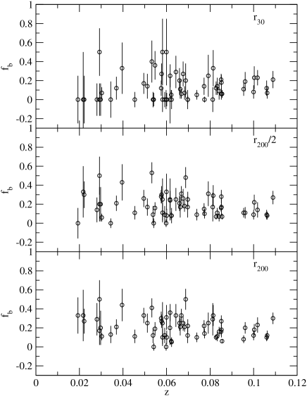
Figure 2: The blue fraction to $M^{*}+1.5$ for all clusters, in all three apertures considered

Inspection of Fig. 2 shows that there is considerable scatter in the derived blue fraction. This is consistent with previous studies of local and X-ray selected samples (Smail et al., 1998; Margoniner et al., 2001; Goto et al., 2003a). We compare the distribution of points with a Gaussian distribution with mean and standard deviation derived from a weighted fit to the data. The distribution shows significant skewness and a $\chi^{2}$ test yields probabilities below 10^-3 that the data points are consistent with a single value of $f_{b}$. This suggests that the scatter observed is a real property of the sample.

We plot the mean values of f_b as a function of the magnitude limit used for all three apertures in Fig. 3. A $t-$test shows that the distributions have significantly different means: the blue fraction increases as a function of radius and as a function of luminosity. This is consistent with previous findings by Margoniner et al. (2001) and Ellingson et al. (2001) and implies that the the blue galaxies are intrinsically faint objects and reside preferentially in the cluster outskirts.

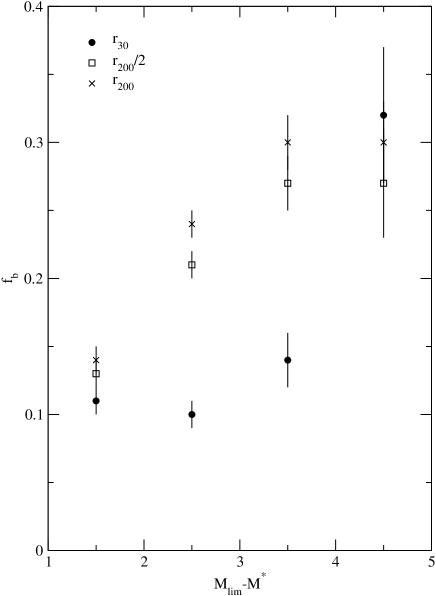
Figure 3: Mean values of the blue fraction as a function of luminosity and aperture

3.2 Dependence on cluster properties

We will next consider how the blue fraction depends on cluster properties derived from our original study (De Propris et al., 2002): Bautz-Morgan type, richness, presence of substructure, velocity dispersion and concentration.

The Bautz-Morgan type measures the dominance of the brightest cluster galaxy relative to the rest of the cluster population. It is used as an indicator of dynamical evolution, where the brightest galaxy evolves via the merger of $M^{*}$ galaxies at the cluster center. Velocity dispersion provides a measure of the cluster mass (assuming the clusters to be virialized) and of the relative speed of galaxy encounters (which is important for some of the mechanisms for the origin of the Butcher-Oemler effect). Richness, as measured from the number of galaxies brighter than $M_{b_{\rm J}}=-19$ (De Propris et al., 2003a), is an indicator of cluster mass and mean density. We consider the probability that a cluster contains substructure, using the Lee-Fitchett statistics (Fitchett, 1988). Although there is no metric to determine the amount of substructure a cluster contains, the probability of its being significantly substructured provides a measure of the amount of recent merging a cluster has undergone and therefore may allow us to estimate how recently the cluster has formed. Finally, we consider the dependence on cluster concentration, defined as

$$C=\log(r_{60}/r_{20})$$

where $r_{20}$ and $r_{60}$ are the radii containing 20% and 60% of the cluster population, respectively.

Fig. 4 shows how the blue fraction (to $M^{*}+1.5$) depends on these five variables. We only plot the case corresponding to $r_{200}/2$ for economy of space, but the results are similar in all three apertures. In no case is there any clear evidence of any dependence of the blue fraction on Bautz-Morgan type, richness, velocity dispersion, probability of substructure or concentration. This is confirmed by a non-parametric Spearman test, which returns low correlation probabilities in all instances.

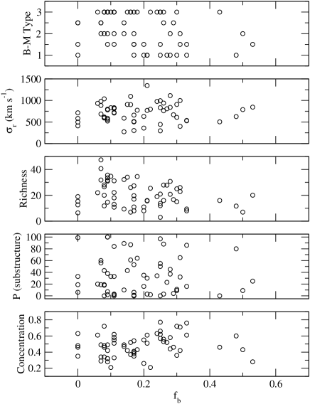
Figure 4: Dependence of the measured blue fraction on cluster properties for the $r_{200}/2$ aperture

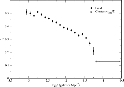
Figure 5: The blue fraction in the general field as a function of local density (filled circles) and the mean for all clusters within $r_{200}/2$ (open square). Density is defined within 8 Mpc spheres as in Croton et al. (2004). For clusters we use the number of galaxies within $r_{200}$ and assume that all cluster members are within this sphere in our calculation of density. Because this is likely to be a slight underestimate, we indicate in the figure that this density is only a lower limit.

3.3 Density dependence in the field

We have selected a sample of field galaxies from the 2dFGRS galaxy redshift survey with the same redshift distribution as the clusters. For each galaxy we derived the local density in an 8 Mpc sphere (Croton et al. 2004). From this sample we determine the blue fraction as a function of local density in Fig. 5.

The blue fraction follows a well defined linear trend, becoming higher in low density regions. This trend can be extended to clusters, whose behaviour is then simply the more extreme version of the relation between $f_{b}$ and local density as observed in the general field.

Galaxies then display a bimodal distribution in colour space, with well-defined red and blue wodges, whose relative populations change with density. This represents a confirmation of the trends observed by the SDSS in their more extensive photometry (Hogg et al., 2003; Blanton et al., 2003b).

It is interesting to compare how the relative star formation rates, as measured from H$\alpha$ equivalent widths, vary with density or with the only properties that, in clusters, appear to affect the blue fraction, luminosity and radius (computing absolute star formation rates is difficult with 2dF data, as the spectra are not easy to flux calibrate, but H$\alpha$ equivalent widths can be used to provide an estimate of the relative star formation rate within the sample). The H$\alpha$ equivalent widths were computed using Gaussian line fitting with a small ($2$ Å) correction for underlying line absorption. No dust extinction correction was carried out. A full description of the procedures used can be found in Lewis et al. (2002), especially their section 2.4.

The variation of H$\alpha$ equivalent width with density, luminosity and radius is shown in Fig. 6 and 7. for red and blue galaxies in both environments. We see that, while the blue fraction changes the mean relative star formation rate does not. The bimodal behaviour observed in the colours extends to the H$\alpha$ equivalent width, as noticed by Balogh et al. (2003). The changes in blue fraction and H$\alpha$ equivalent width as a function of density are due to changes in the relative fractions of quiescent and star forming galaxies.

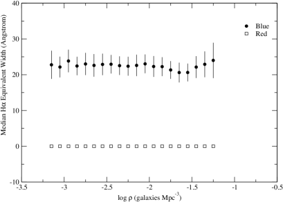
Figure 6: Median H$\alpha$ equivalent widths (in Angstroms) for blue and red galaxies in the field as a function of density. Errors are interquartile means. The errors for the red galaxies are smaller than the symbols.

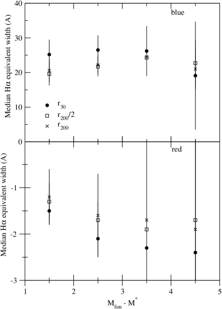
Figure 7: Median H$\alpha$ equivalent widths (as in Fig. 6) for blue and red galaxies in clusters as a function of luminosity and radius. Errors are interquartile means.

4 Discussion

We have determined the fraction of blue galaxies in a sample of nearby clusters and in the general field at the same redshift. Although the blue fraction varies considerably from cluster to cluster, we find that the variation is a real property of the sample and not due to statistical noise.

The mean value of the blue fraction is $0.11\pm 0.01$ for galaxies within $r_{30}$ and $0.13\pm 0.01$ for galaxies within $r_{200}/2$. These are higher than the value of $0.03\pm 0.09$ from Margoniner & de Carvalho (2000), $\sim 0.07$ from Margoniner et al. (2001) and $\sim 0.07$ from Pimbblet et al. (2002) at $z<0.11$, although they are within the errors. One possibility for this discrepancy lies in the possibility of blue interlopers from the field population being included in our redshift sample (Diaferio et al., 2001). We have calculated the level of contamination by integrating the field luminosity function of Madgwick et al. (2002) over the appropriate luminosity range and within the pseudo-volume defined by the aperture used and the range in velocities spanned by cluster galaxies. The blue fraction for this sample was calculated from our density-dependent blue fraction. The average level of contamination is $0.08\pm 0.06$ but this depends critically on assumptions concerning the mean density of galaxies in cluster outskirts (which influence both the normalization and the fraction of blue interlopers as per Fig. 5). In addition, there are contributions to the error from both Poisson and clustering statistics. The number of blue galaxies is, in any case, small and therefore the level of contamination is uncertain and the error in its estimate quite large. We therefore ignore the issue of possible contamination of our spectroscopic sample of cluster members.

• A first conclusion to be drawn from the derived blue fractions is that few clusters have $f_{b}>40\%$ and none has $f_{b}>60\%$ .

  Since this sample of clusters is, at least to first order, complete and volume limited, it represents a fair sampling of the range of blue fractions encountered in cluster environments. By contrast, samples of clusters at high redshift contain at least a few objects with blue fractions in excess of 40% (Fairley et al. 2002, La Barbera et al. 2003 and references therein). This would suggest that the observed evolution is real: contamination in our sample (if real) should only make the local blue fraction lower, while high redshift clusters are drawn from the high richness envelope that contains few local clusters with high $f_{b}$. However, it is possible that optically selected clusters at high redshift tend to contain higher fractions of blue galaxies because these make them more conspicuous in blue plates.
  

• The blue fraction appears to depend on the luminosity limit and cluster centric radius used (Fig. 3), as previously found by Margoniner & de Carvalho (2000) and Ellingson et al. (2001).

  This behaviour is similar to that observed for dwarf galaxies in Coma and Abell 2218: Pracy et al. (2003) have shown that dwarfs have a steeper luminosity function at larger cluster centric radii and are preferentially found at large distances from the cluster core, with these trends being stronger for the faintest dwarfs. Similar trends may have been observed for galaxies in the Coma cluster (Beijersbergen et al., 2002) and appear to persist in the $z\sim 0.4$ CNOC sample. To the extent that present-day clusters and their populations represent proxies for high redshift objects, these observations imply that a proportion of the blue galaxies are intrinsically low luminosity objects.
  

• There is no dependence of the blue fraction on cluster properties (Fig. 4). The lack of correlation of the blue fraction with cluster properties suggests that the star formation rate, or its decrease, is not related to the large scale structure: therefore, mechanisms which involve cluster-wide effects, such as ram stripping by the cluster gas, tides, which depend on the cluster mass, or harassment, whose efficiency is proportional to velocity dispersion, are disfavoured by the present study, as well as other explanations that depend on processes specific to the cluster environment. However, as Balogh et al. (2003) show, the star formation rate is affected by local processes and close interactions are a viable mechanism for the origin of the blue fraction.

  The above is apparently in contrast with some previous studies: Metevier et al. (2000) claim that clusters containing large amounts of substructure have higher blue fractions and interpret this in terms of a shock model during collisions of subclusters. However, their result is based on three clusters and may not be valid for the general population. Margoniner et al. (2001) and Goto et al. (2003a) suggest that the blue fraction depends on richness. One possibility is that, since they use a fixed 0.7 Mpc aperture, and given the radial dependence observed in Fig. 3, that a spurious richness dependence may be induced by aperture effects. We have derived blue fractions for a 0.7 Mpc aperture in our clusters and tested for correlation with richness but failed to detect a significant signal. Similarly, we failed to detect any correlation with richness if we use the same luminosity range as Margoniner et al. (2001). However, we see in Fig. 4 that rich clusters tend not to have large blue fractions and we also observe that the blue fraction in the 0.7 Mpc aperture shows large scatter. If the sample used by Margoniner et al. (2001) and Goto et al. (2003a) is biased towards richer clusters at high redshift, the combination of these two effects may produce a spurious correlation.
  

• We observe that the blue fraction exhibits a strong dependence with local density in the general field (Fig. 5) and that the cluster value represents a continuation of this trend to higher density regimes.

  This suggests that the same processes are responsible for the Butcher-Oemler effect in all environments and that these mechanisms vary smoothly as a function of density. Again, this implies that cluster-specific processes are not likely causes of changes in the blue fraction, but local mechanisms whose efficiency varies smoothly with density, such as interactions (Lavery & Henry, 1988; Couch et al., 1998), may be viable explanations.
  

• The relative star formation rate for the blue galaxies does not appear to decrease as a function of density (Fig. 6) or as a function of luminosity or radius in clusters (Fig. 7).

  This implies that changes in the blue fraction are solely due to changes in the relative fractions of red (quiescent) and blue (star-forming) galaxies. The trends we observe can be roughly reproduced by using the density-dependent luminosity functions of Croton et al. (2004) for early- and late-type galaxies and the type-dependent cluster luminosity functions of De Propris et al. (2003a) and simply assuming that early-type galaxies are red and late types are blue. This suggests that the simple model presented in De Propris et al. (2003a), where galaxies simply moved between spectral types without number or luminosity evolution, provides, heuristically, a good representation of galaxy evolution.
  

  One possible caveat is that, by selecting blue galaxies, we have automatically selected for galaxies with H$\alpha$ emission, while morphologically selected samples show declining star formation rates as a function of density (Gomez et al., 2003; Goto et al., 2003b). However, the observation that blue cluster galaxies have the same H$\alpha$ equivalent width as their counterparts in the field is non-trivial, because lower (but non-zero) star formation rates will lead to weaker H$\alpha$ emission, while the colour would remain blue by our definition. This is in contrast, for instance, with models where galaxies are ‘choked’ in clusters (Balogh et al., 2000).

The above argues for a model where star formation declines over relatively short timescales, leading to the bimodal distribution in H$\alpha$ observed by Balogh et al. (2003), and galaxy colours evolve quickly to the red envelope, producing the colour bimodality observed here and in the SDSS (Hogg et al., 2003; Blanton et al., 2003b). As in De Propris et al. (2003a) this is possible if the optical colour is dominated by the young population but the majority of light is provided by the underlying old stars, so that once the star formation is extinguished galaxy colours quickly evolve on to the passive locus. Shioya et al. (2002) have shown that truncating the star formation of spiral galaxies in the field leads them on to the colour-magnitude relation defined by the Coma E/S0 galaxies, but that this process is inefficient for the more massive galaxies and is viable only for low mass spirals. When we consider the radial and luminosity trends, one possible interpretation is that a large fraction of the blue galaxies are actually dwarfs undergoing episodes of star formation, as also suggested by a number of other lines of evidence (Rakos et al., 1997; Couch et al., 1998; De Propris et al., 2003b). However, we caution the reader that since our sample of cluster and field galaxies is local, we cannot properly discuss the origin of the blue fraction at higher redshift.

A complication in interpreting these data is that the observed correlations of $f_{b}$ and H$\alpha$ with density on large scales imply that the environment today is not affecting the properties of the population and therefore we are unable to observe galaxy evolution in progress but just its end result. This implies that identifying the mechanisms responsible for the Butcher-Oemler effect in the local universe is problematic. Surveys at intermediate redshifts (e.g. DEEP2, VIMOS) may be able to witness the main phases of galaxy evolution.

References

- (1)
- (2)
- Andreon & Ettori (1999) Andreon S., Ettori S. 1999, ApJ, 516, 647
- Armstrong & Kung (1978) Armstrong R. D., Kung M. T. 1978, Appl. Stat. 27, 363
- Balogh et al. (2000) Balogh M. L., Navarro J. F., Morris S. 2000, ApJ, 540, 113
- Balogh et al. (2003) Balogh M. L. et al. 2003, MNRAS, in press
- Beijersbergen et al. (2002) Beijersbergen M., Hoekstra H., van Dokkum P., van der Hulst T. 2002, MNRAS, 329, 385
- Blanton et al. (2003a) Blanton M. R. et al. 2003a, AJ, 125, 2348
- Blanton et al. (2003b) Blanton M. R. et al. 2003b, ApJ, 594, 186
- Bruzual & Charlot (2003) Bruzual G., Charlot S. 2003, MNRAS, 344, 1000
- Butcher & Oemler (1984) Butcher H., Oemler A. E. 1984, ApJ, 285, 426
- Carlberg et al. (1997) Carlberg R., Yee H. K. C., Ellingson E. 1997, ApJ, 478, 462
- Cooperstock et al. (1998) Cooperstock F. I., Faraoni V., Vollick D. 1998, ApJ, 503, 61
- Couch et al. (1994) Couch W. J., Ellis R. S., Sharples R. M., Smail I. 1994, ApJ, 430, 121
- Couch et al. (1998) Couch W. J., Barger A. J., Smail I., Ellis R. S., Sharples R. M. 1998, ApJ, 497, 188
- Croton et al. (2004) Croton D. et al. 2004, MNRAS, submitted
- De Propris et al. (2002) De Propris R. et al. 2002, MNRAS, 329, 87
- De Propris et al. (2003a) De Propris R. et al. 2003a, MNRAS, 342, 725
- De Propris et al. (2003b) De Propris R., Stanford S. A., Eisenhardt P. R., Dickinson M. 2003b, ApJ, 598, 20
- Diaferio et al. (2001) Diaferio A., Kauffmann G., Balogh M., White S. D. M., Schade D., Ellingson E. 2001, MNRAS, 323, 999
- Ellingson et al. (2001) Ellingson E., Lin H., Yee H. K. C., Carlberg R. 2001, ApJ, 547, 609
- Fairley et al. (2002) Fairley B. W., Jones L. R., Wake D. A., Collins C. A., Burke D. J., Nichol R. C., Romer A. K. 2002, MNRAS, 330, 755
- Fitchett (1988) Fitchett M. 1988, MNRAS, 230, 161
- Gnedin (2003) Gnedin O. Y. 2003, ApJ, 582, 141
- Gomez et al. (2003) Gomez P. L. et al. 2003, ApJ, 584, 210
- Goto et al. (2003a) Goto T. et al. 2003a, PASJ, 55, 739
- Goto et al. (2003b) Goto T. et al. 2003b, PASJ, 55, 757
- Hambly et al. (2001) Hambly N. C., Irwin M. J., McGillivray H. T. 2001, MNRAS, 326, 1295
- Hogg et al. (2003) Hogg D. W. et al. 2003, ApJ, 585, L5
- Hogg et al. (2004) Hogg D. W. et al. 2004, ApJ, 601, L29
- Holden et al. (2002) Holden B. P., Stanford S. A., Squires G. K., Rosati P., Tozzi P., Eisenhardt P., Spinrad H. 2002, AJ, 124, 33
- La Barbera et al. (2003) La Barbera F., Busarello G., Massarotti M., Merluzzi P., Mercurio A. 2003, A&A, 409, 21
- Lavery & Henry (1988) Lavery H. J., Henry J. P. 1988, ApJ, 330, 596
- Lewis et al. (2002) Lewis I. J. et al. 2002, MNRAS, 334, 673
- Madgwick et al. (2002) Madgwick D. S. et al. 2002, MNRAS, 333, 133
- Margoniner & de Carvalho (2000) Margoniner V. E., de Carvalho R. R. 2000, AJ, 119, 1562
- Margoniner et al. (2001) Margoniner V. E., de Carvalho R. R., Gal R. R., Djorgovski S. G. 2001, ApJ, 548, L143
- Metevier et al. (2000) Metevier A. J., Romer A. K., Ulmer M. P. 2000, AJ, 119, 1090
- Moore et al. (1996) Moore B., Katz N., Lake G., Dressler A., Oemler A. 1996, Nature, 379, 613
- Newberry et al. (1988) Newberry M. V., Kirshner R. P., Boroson T. A. 1988, ApJ, 335, 629
- Pimbblet et al. (2002) Pimbblet K. A., Smail I., Kodama T., Couch W. J., Edge A. C., Zabludoff A. I., O’Hely E. 2002, MNRAS, 331, 333
- Pracy et al. (2003) Pracy M., De Propris R., Couch W. J., Driver S. P., Nulsen P. E. J. 2003, MNRAS, submitted
- Rakos et al. (1997) Rakos K. D., Odell A. D., Schombert J. M. 1997, ApJ, 490, 194
- Shioya et al. (2002) Shioya Y., Bekki K., Couch W. J., De Propris R. 2002, ApJ, 565, 223
- Smail et al. (1998) Smail I., Edge A. C., Ellis R. S., Blandford R. D. 1998, MNRAS, 293, 124