Particle Acceleration in an Evolving Network of Unstable Current Sheets

Abstract

We study the acceleration of electrons and protons interacting with localized, multiple, small-scale dissipation regions inside an evolving, turbulent active region. The dissipation regions are Unstable Current Sheets (UCS), and in their ensemble they form a complex, fractal, evolving network of acceleration centers. Acceleration and energy dissipation are thus assumed to be fragmented. A large-scale magnetic topology provides the connectivity between the UCS and determines in this way the degree of possible multiple acceleration. The particles travel along the magnetic field freely without loosing or gaining energy, till they reach a UCS. In a UCS, a variety of acceleration mechanisms are active, with the end-result that the particles depart with a new momentum. The stochastic acceleration process is represented in the form of Continuous Time Random Walk (CTRW), which allows to estimate the evolution of the energy distribution of the particles. It is found that under certain conditions electrons are heated and accelerated to energies above $1\,$MeV in much less than a second. Hard X-ray (HXR) and microwave spectra are calculated from the electrons’ energy distributions, and they are found to be compatible with the observations. Ions (protons) are also heated and accelerated, reaching energies up to 10 MeV almost simultaneously with the electrons. The diffusion of the particles inside the active region is extremely fast (anomalous super-diffusion). Although our approach does not provide insight into the details of the specific acceleration mechanisms involved, its benefits are that it relates acceleration to the energy release, it well describes the stochastic nature of the acceleration process, and it can incorporate the flaring large-scale magnetic topology, potentially even its temporal evolution.

1 Introduction

Solar flares remain, after almost one hundred years of intense study, an unsolved problem for astrophysics. We define as flare the sporadic transformation of magnetic energy to (1) plasma heating, (2) particle acceleration, and (3) plasma flows. It seems that the total magnetic energy released in a single flare is not equally spread to all three components. The energetic particles carry a very large fraction of the total energy released during a flare, reaching sometimes up to $50\%$ (Saint-Hilaire and Benz, 2002).

Modeling the explosive energy release requires methods that can treat simultaneously the large scale magnetic field structures and the small-scale dissipation events. The convection zone actively participates in the formation and evolution of large scale structures by rearranging the position of the field lines and at the same time it adds new magnetic flux (emerging flux) and new stresses to the existing topologies. The loss of stability of several loop-like structures forms large scale disturbances (CME), which further disturb the pre-existing and so-far stable large scale structures. In this way, the 3-D magnetic topologies are constantly forced away from the potential state (if they ever reach one) due to slow or abrupt changes in the convection zone. All these non-potential magnetic stresses force the large-scale magnetic topology to form short-lived, small-scale magnetic discontinuities in order to dissipate the excess energy in localized current sheets. This conjecture was initially proposed by Parker (1988), and subsequently it was modeled using 3-D MHD numerical simulations by many researchers (see for example the work of Nordlund & Galsgaard, 1996). We emphasize here that the concept of sudden formation of a distribution of unstable discontinuities inside a well organized large-scale topology has not been appreciated or used extensively enough to model the solar flare phenomenon.

The scenario of spatially distributed, localized, small-scale dissipation, which moreover evolves in time, is not least supported by the observations which indicate highly fragmented energy dissipation and particle acceleration processes. There is strong evidence that narrow-band milli-second spike-emission in the radio range is directly associated to the primary energy release events. The emission itself of the radio-spikes is fragmented in space and time, as is seen in radio-spectrograms and in spatially resolved observations. It must thus be concluded that also the energy release process is fragmented in space and time, to at least the same degree as is the radio spike-emission (see Benz, 2003). Also type III burst radio-emission, caused by electron beams escaping from flaring regions, exhibits fragmentation as a strong characteristic (e.g. Benz, 1994). It is a too simple interpretation of the available data that the large scale structures seen have a relatively simple topology down to all scales.

One approach which is capable to capture the full extent of this interplay of highly localized dissipation in a well-behaved large scale topology (’sporadic flaring’) is based on a special class of models which use the concept of Self-Organized Criticality (SOC; Bak et al, 1987). The main idea is that active regions evolve by the continuous addition of new or the change of existing magnetic flux on an existing large scale magnetic topology, until at some point(s) inside the structure magnetic discontinuities are formed and the currents associated with them reach a threshold. This causes a fast rearrangement of the local magnetic topology and the release of the excess magnetic energy at the unstable point(s). This rearrangement may in-turn cause the lack of stability in the neighborhood, and so forth, leading to the appearance of flares (avalanches) of all sizes that follow a well defined statistical law (Lu and Hamilton, 1991; Lu et al., 1993; Vlahos et al., 1995; Isliker et al., 2000, 2001), which agrees remarkably well with the observed flare statistics (Crosby, Aschwanden and Dennis, 1993).

The modeling of the solar atmosphere cannot be done exclusively with the use of high-resolution MHD numerical codes. The small scale discontinuities easily give rise to kinetic instabilities and anomalous resistivity, which play a very important role, they dramatically change the evolution of even the large scale structures. On the other hand, numerical codes following the evolution of charged particles in idealized, non-evolving, large-scale current-sheets also fail to capture the spatio-temporal evolution of the magnetic energy dissipation. The extraordinary efficiency of particle acceleration during solar flares questions the use of ideal MHD for the description of flares, since it misses kinetic plasma effects, which yet play a major role in the energy dissipation process and for the local state of the plasma. The coupling of the large scale and the small scale is extremely difficult to handle, not only in solar physics but in physics in general, and it is the main reason for not having resolved the solar flare problem for so many years (Cargill, 2002).

Our inability to describe properly the coupling between the MHD evolution and the kinetic plasma aspects of the driven flaring region is the main reason behind our lack of understanding of the mechanism(s) which causes the acceleration of high energy particles. Let us now define more accurately the so called ‘acceleration problem’. We need to understand the mechanism(s) which accelerate electrons and ions in relatively large numbers to energies well above the relativistic regime on a short time scale with specific energy-spectra for the different isotopes and charge states.

Let us summarize very briefly the main observational constraints for the acceleration processes in solar flares.

Electron energies well in excess to 100 keV, and occasionally up to tens of MeV, are inferred. Electrons reach $100$keV in $<1$s and higher energies in a few seconds. The number of electrons required above 20 keV is large for x-class flares and can reach up to $10^{38}$ electrons per second, although this number is model dependent and not very accurate (see e.g. Miller et al., 1997). The observed spectra in the hard X-rays can be fitted with single or double power-laws, combined often — but not always — with a thermal emission spectrum at the lowest energies (Holman, 2003; Holman et al, 2003; Piana et al., 2003). The spectra in the microwaves roughly show a power-law decay at high frequencies (Holman, 2003).

Ions (especially protons) are inferred to have energies above $1\,$MeV and up to $1\,$GeV per nucleon. The 10 MeV ions are accelerated on the same time scales as the electrons, with the high energy ions delayed up to $10\,$s. The total number of ions accelerated may carry the same energy as the electrons. The continuous component of the $\gamma$-ray spectra are usually power laws. An important finding is the massive enhancement of ${}^{3}_{2}$He in very impulsive flares (see e.g. Miller et al., 1997).

Acceleration mechanisms: Numerous books and reviews have been devoted to the challenging problem of particle acceleration (Heyvaerts, 1981; Vlahos et al., 1984; Melrose, 1992; Vlahos, 1994; Kirk, 1994; Vlahos, 1996; Kuijpers, 1996; Miller et al., 1997). The proposed models usually address parts of the problem, and almost all acceleration mechanisms have no clear connection to the large-scale topology and to the magnetic energy release mechanism(s). The most prominent mechanisms are shock waves (Holman and Pesses, 1983; Blandford and Eichler, 1987; Ellison and Ramaty, 1985; Decker, 1988), MHD turbulence (Fermi, 1949; Miller and Roberts, 1995), and DC electric fields (Benka and Holman, 1992; Moghaddam-Taaheri et al., 1985; Moghaddam-Taaheri and Goertz, 1990).

Mixing acceleration mechanisms: Several inquiries have been made in which different acceleration mechanisms had been mixed.

Decker and Vlahos (1986) analyzed the role of Shock Drift Acceleration (SDA) when the shock is surrounded by a turbulent spectrum. As we already mentioned, the SDA is fast but not efficient since the particles drifting along the shock-surface’s electric field quickly leave the shock. The presence of turbulence reinforces the acceleration process by providing a magnetic trap around the shock surface and forcing a particle to return many times to the shock surface. The particle leaves the shock surface, travels a distance $s_{i}$ inside the turbulent magnetic field, returns back to the shock surface with velocity $v_{i}$, drifts a distance $l_{i}$ along the shock electric field $E_{sc}$, changing its momentum by $\Delta p_{i}\sim E_{sc}\cdot(l_{i}/v_{i})$, it escapes again, travels a distance $s_{i+1}$ before returning back to the shock and drifting along the electric field, in other words, the acceleration-cycle has begun again. The process repeats itself several times before the particle gains enough energy to escape from the turbulent trap around the shock surface. Let us note some very important characteristics of this acceleration: (1) The distances $s_{i}$ traveled by the particle before returning back to the shock are only indirectly relevant to the acceleration, they basically delay the process and influence the overall timing, i.e. the acceleration time, another important parameter of the particle acceleration process. (2) The energy gain depends critically on the lengths $l_{i}$ the particle drifts along the shock surface, in a statistical sense though, i.e. on the distribution of the $l_{i},\,i=1,2,3\,...$. (3) The times $\tau_{i}$ a particle spends on the shock surface are again crucial for the energy gain, and also, together with the $s_{i}$, for the estimation of the acceleration time. (4) For the total acceleration problem, which concerns the energies reached and the times needed to reach them, all three variables, $s_{i},\,l_{i},\,\tau_{i}$, are of equal importance.

Ambrosiano et al. (1998) discussed a similar problem, placing a current sheet into a region of Alfvénic turbulence. Also here, the ability of the associated DC electric field to accelerate particles is enhanced by the presence of the MHD turbulence. The acceleration process is again of a cyclic nature, as in the case of turbulent SDA, and the process is again characterized by the three variables $s_{i},\,l_{i},\,\tau_{i}$. The turbulent current sheet has several avenues to enhance the acceleration-efficiency since the plasma inflow is dynamically driven and causes a variety of new and still unexplored phenomena. Arzner (2002) analyzed the mixture of stationary MHD turbulence with a DC electric field. The trapping of the particles inside the turbulent magnetic field causes a new ‘collision scale’, and, in some circumstances, acceleration becomes dependent on an alternative ’Dreicer field’, in which particle collisions are replaced by collisions with magnetic irregularities. Actually also the diffusive shock acceleration described above is of a mixed type, having as elements a shock and magnetic turbulence, although turbulence plays a more passive role of just scattering the particles. It seems that most acceleration mechanisms are more or less of a mixed type.

We can conclude that the mixture of mechanisms enhances the acceleration-efficiency and removes some of the draw-backs attached to the different, isolated mechanisms. A second, main conclusion we draw is that cyclic processes, e.g. through trapping around the basic accelerators, are important elements — if not the presupposition — of efficient and fast acceleration in space plasmas.

Can the UCS naturally provide the unification of all the above mechanisms ? Unstable Current Sheets (UCS) are the regions where magnetic energy is dissipated, and it is natural to ask if they can become the actual source of the energetic particles. According to the existing understanding of UCSs, several potential mechanisms for particle acceleration co-exist at a UCS. Plasma flows driving turbulence, shock waves, and DC electric fields are expected to appear simultaneously inside and around a driven and evolving UCS. If the UCS is located in the middle of a turbulent magnetic topology, all these phenomena will be enhanced and the sporadic external forcing of the plasma inflow into the UCS will create bursts of sporadic acceleration. The scenario of a single UCS currently enjoys very large popularity (e.g. Litvinenko, 2003; Fletcher and Martens, 1998; Martens, 1988), and the question is: Can one single UCS be the answer to the acceleration problem ?

We believe that this is impossible since a single, isolated UCS must be enormously large $(10^{9}\times 10^{9}\times 10^{5}$ m), remain stationary for a long time, and continuously accelerate particles with extreme efficiency in order to provide the required numbers of accelerated particles and the observed acceleration times. From the Earth’s magnetic tail, it is known that large UCS break up quickly, creating a network of smaller scale UCS, with a specific probability distribution $P(l)$ of their characteristic scales, a process which just is a manifestation of turbulence (Angelopoulos et al., 1999). The formation of a large scale helmet above certain loops, driven by erupting filaments cannot be excluded entirely and represents a special class of very energetic phenomena (Masuda et al., 1992). We though believe that such a current sheet breaks down on a very short time scale, and the formation of smaller scale current sheets will be unavoidable. Eventually, even in this very special occasion the acceleration probably takes place in an environment similar to the one discussed in this article.

There is a second reason, based on a result on the statistics of flares, for questioning the idea of a single, large-scale UCS that is associated with just one or at most two loops, as in the scenario of the sometimes called ’standard model’ (see e.g. Shibata et al., 1995). Wheatland (2000) determined the frequency-distributions in total emitted energy of flares occurring in the same, individual active region (number of flares per unit energy), and they find featureless power-law distributions, extending over many decades. If a single UCS would be the basic mechanism behind a flare, then the energy output must be expected to be related to the physical properties of the individual active region, e.g. to the linear dimensions of the active region and the associated UCS, so that it is at least difficult to imagine how a single-site reconnection model could be able to produce a featureless energy distribution that extends over many decades.

From single to multiple, small-scale UCS acceleration: Our attempt in this article is to take advantage of the positive properties of isolated UCS as accelerators, but at the same time to assume that the dissipation happens at multiple, small-scale sites.

The 3-D magnetic topology, driven from the convection zone, dissipates energy in localized UCS, which are spread inside the coronal active region, providing a natural fragmentation for the energy release and a multiple, distributed accelerator. In this way, the magnetic topology acts as a host for the UCS, and the spatio-temporal distribution of the latter defines the type of a flare, its intensity, the degree of energization and acceleration of the particles, the acceleration time-scales etc. Evolving large-scale magnetic topologies provide a variety of opportunities for acceleration which is not restricted to flares, but can also take place before a flare, and after a flare, being just the manifestation of a more relaxed, but still driven topology. Depending thus on the level to which the magnetic topology is stressed, particles can be accelerated without a flare to happen, and even long-lived acceleration in non-flaring active regions must be expected to occur. Consequently, the starting point of the model to be introduced below is a driven 3-D magnetic topology, which defines a time-dependent spatial distribution of UCS inside the active region. In this article, we will focus on the interaction of the UCS with particles. The details of the mechanisms involved in the acceleration of particles inside the UCS are not essential in a stochastic modeling approach.

Ideas related to the basic approach of this article have been presented earlier (Anastasiadis and Vlahos, 1991; Vlahos, 1993; Anastasiadis and Vahos, 1994; Anastasiadis et al., 1997), but remained conceptually simpler, they left many points open for future development, being not that general and complete as approaches as the model we present here. In the approach we follow here, we make extensive use of new developments in the theory of SOC models for flares. Also taken into account are ideas from the theory of Complex Evolving Networks (Albert and Barabasi, 2002; Dorogovtsev and Mendest, 2002), adjusted though to the context of plasma physics: The spatially distributed, localized UCS can be viewed as a network, whose ’nodes’ are the UCS themselves, and whose ’edges’ are the possible particle trajectories between the nodes (UCS). The particles are moving around in this network, forced to follow the edges, and undergoing acceleration when they pass by a node (see also Fig. 2). The network is complex in that it has a non-trivial spatial structure, and it is evolving since the nodes (UCS) are short-lived, as are the connectivity channels, which ever change during the evolution of a flare. This instantaneous connectivity of the UCS is an important parameter in our model, it determines to what degree multiple acceleration is imposed onto the system, which in turn influences the instantaneous level of energization and the acceleration time-scale of the particles.

In this article, we introduce a stochastic, multiple acceleration model for solar flare particle acceleration. We assume an ensemble of unstable current sheets (UCS), distributed in space in such a way that it reflects a relatively simple large scale topology in which turbulence at small scales is developing. Concretely, the UCS in their ensemble form a fractal, as it is the case in the SOC models (Isliker & Vlahos, 2003b; McIntosh et al., 2002). Particles move erratically around, and occasionally enter a UCS in which they undergo acceleration. The acceleration process is taken as a simple DC electric field mechanism. The basic approach of the model is a combined random walk in position- and momentum-space. The frame-work we introduce is such that potentially all multiple acceleration models can be formulated in this frame-work, as long as the acceleration takes place in spatially localized, disconnected, small-scale regions. Our main interest here is in the diffusion, acceleration, and heating of the electrons. We will follow the evolution of the kinetic energy distribution in time and calculate from these distributions the hard X-ray (HXR) and microwave spectra, which can be compared to the observations. Moreover, we will shortly inquire the case of ion heating and acceleration.

The basic elements of our model are presented in Section 2. In section 3, we present some of our results, and in section 4 we discuss our findings and propose ways for continuing the exploration of the problem along the path of our modeling approach. A conclusion is presented in section 5.

2 The model

In the model we propose in this article, a 3-D large scale magnetic topology, close to the structures estimated by force-free extrapolations of the photospheric magnetic fields, is the back bone of the system (see Fig. 1(a)). The magnetic field lines are the carriers of the high energy particles. The UCS, which basically are magnetic discontinuities, appear sporadically inside the large scale magnetic topology, and they represent the dissipation areas of the turbulent system (see Fig. 1(d)). The characteristics of the UCS, such as size, energy content, etc., are different from UCS to UCS, following probabilistic laws which in principle should be dictated by the data, most of them though are not directly observable. The UCS are assumed to be small-scale regions, distributed over space in a complex way. We thus implement the scenario of fragmented energy release, based on Parker’s original conjecture (Parker, 1988) and on the observational evidence of fragmentation in radio spike emission (see e.g. Benz, 2003), and in type III radio-emission (e.g. Benz, 1994).

One way of modeling the appearance, disappearance, and spatial organization of UCS inside a large scale topology is with the use of the Extended Cellular Automaton (X-CA) model (Isliker et al., 1998, 2000, 2001). Fig. 1 illustrates some basic features of the X-CA model.

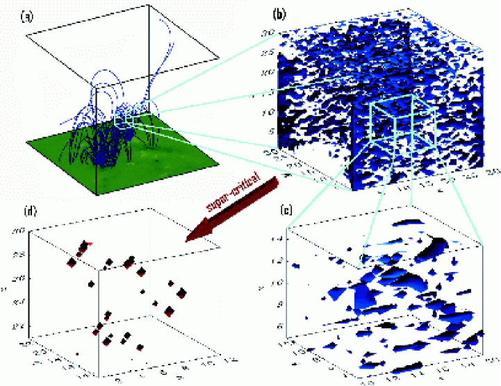
Figure 1: (a) Simulated magnetogram of a photospheric active region and force-free magnetic field-lines, extrapolated into the corona (generated by the model of Fragos et al. (2003)). — (b) Sub-critical current iso-surfaces in space, as yielded by the X-CA model, which models a sub-volume of a coronal active region. — (c) The same as (b), zoomed. (d) Temporal snap-shot of the X-CA model during a flare, showing the spatial distribution of the UCS (super-critical current iso-surface) inside the complex active region. The UCS form a fractal, and they are connected through large-scale magnetic field lines. The connectivity between the UCS is an important ingredient of the acceleration mechanism proposed.

The X-CA model has as a core a cellular automaton model of the sand-pile type and is run in the state of Self-Organized Criticality (SOC). It is extended to be fully consistent with MHD: The primary grid variable is the vector-potential, and the magnetic field and the current are calculated by means of interpolation as derivatives of the vector potential in the usual sense of MHD, guaranteeing $\nabla\cdot\vec{B}=0$ and $\vec{J}=(4\pi/c)\cdot\nabla\times\vec{B}$ everywhere in the simulated 3-dimensional volume. The electric field is defined as $\vec{E}=\eta\vec{J}$, with $\eta$ the resistivity. The latter usually is negligibly small, but if a threshold in the current is locally reached ($|\vec{J}|>J_{cr}$), then current driven instabilities are assumed to occur, $\eta$ becomes anomalous in turn, and the resistive electric field locally increases drastically. These localized regions of intense electric fields are the UCS in the X-CA model.

The X-CA model yields distributions of total energy and peak flux which are compatible with the observations. The UCS in the X-CA form a set which is highly fragmented in space and time, the individual UCS are small scale regions, varying in size, and are short-lived (see Fig. 1(d)). They do not form in their ensemble a simple large scale structure, but they form a fractal set with fractal dimension roughly $D_{F}=1.8$ (Isliker & Vlahos, 2003b; McIntosh et al., 2002). The individual UCS also do usually not split into smaller UCS, but they trigger new UCS in their neighborhood, so that different chains of UCS travel through the active region, triggering new side-chains of UCS on their way.

Following the picture we have from the X-CA model, we consider in this article that the UCS act as nodes of activity (localized accelerators) inside a passive 3-D large scale magnetic topology. The UCS are short lived and appear randomly inside the large scale magnetic topology when specific conditions for instability are met. The sketch in Fig. 2 illustrates the situation.

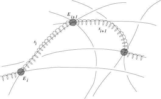
Figure 2: Sketch of the basic elements of the considered model: A particle (spiraling line) follows basically the magnetic field lines (solid lines), undergoing though also drifts, and travels in this way freely a distance $s_{i}$, until it enters a UCS (filled circles), where it is accelerated by the associated effective DC electric field $E_{i+1}$. After the acceleration event, the particle again moves freely until it meets a new UCS.

Modeling this dynamic accelerator requires the knowledge of three probability density functions:

(1) The probability density $P_{1}(s)$ defines the distances a charged particle travels freely in-between two subsequent encounters with a UCS. The series of distances $s^{(j)}_{1},s^{(j)}_{2},...s^{(j)}_{n},...$, generated by the probability density $P_{1}(s)$, characterizes the trajectory of the $j$th particle in space. Every particle follows a different characteristic path.

The probability density $P_{1}(s)$ relates the particle acceleration process to the large scale topology by implicitly representing the effects of the topology (the magnetic topology itself does not appear explicitly in the model). This aspect was never taken into account in previous acceleration models.

(2) The probability density $P_{2}(E)$ provides the effective electric field $E^{(j)}_{i}$ acting on the $j$th particle for the effective time $\tau^{(j)}_{i}$ it spends inside the $i$th UCS. Particles follow very complicated trajectories inside the UCS. They may be accelerated by more than one acceleration mechanisms, but what actually is important for our model is the final outcome, i.e. we characterize a UCS as a simple input-output system, in which an effective DC electric field is acting. We assume thus that the effective action of a UCS is to increase a particle’s momentum by $\Delta\vec{p}^{(j)}_{i}=e\,\vec{E}^{(j)}_{i}\,\tau^{(j)}_{i}$.

(3) Finally, for the third probability, we have two alternative choices: either we give the probability density $P_{3a}(\tau)$ of the effective times $\tau^{(j)}_{i}$ a UCS interacts with a charged particle, or we prescribe the probability density $P_{3b}(\ell)$ of the effective acceleration lengths $\ell^{(j)}_{i}$, i.e.  the lengths of the trajectories along which the particles are accelerated.

The probabilities $P_{1}$, $P_{2}$, and $P_{3}$ (either $P_{3a}$ or $P_{3b}$) are actually dependent on time, they must be assumed to change in the course of a flare, reflecting the changes in the overall density and connectivity of the UCS — the flaring active region is an evolving network of UCS, whose instantaneous state determines the instantaneous intensity of the flare. We will though concentrate in our modeling on a short time during a flare, typically one second, so that we can assume the state of the active region not to change significantly, and $P_{1}$, $P_{2}$, and $P_{3}$ can be considered independent of time.

We will show next that the above probabilities define the charged particle dynamics inside the flaring region.

2.1 Charged particle dynamics

The particle $j$ starts with initial momentum $\vec{p}^{(j)}_{0}$ from the initial position $\vec{r}^{(j)}_{0}=0$ at time $t=0$. The initial momentum $\vec{p}^{(j)}_{0}$ is such that the corresponding velocity $|\vec{v}^{(j)}_{0}|$ is drawn at random from the tail of a Maxwellian, $|\vec{v}^{(j)}_{0}|\geq v_{th}$, with $v_{th}$ the thermal velocity. The particle is assumed to find itself in the neighborhood of a UCS at time $t=0$, enters it immediately and undergoes a first acceleration process.

During an interaction with a UCS, the particle’s momentum in principle evolves according to

$$\frac{d\vec{p}^{(j)}}{dt}=e\vec{E}+\frac{e}{c}\vec{v}^{(j)}\times\vec{B}$$ (1)

where $\vec{p}^{(j)}=\gamma m\vec{v}^{(j)}$ is the particle’s relativistic momentum ($\gamma=1/\sqrt{1-v^{2}/c^{2}}$, with $v=|\vec{v}^{(j)}|$), $e$ is the charge of the particle, and $c$ the speed of light. Inside the UCS, $\vec{E}$ and $\vec{B}$ are complex functions of time along the particle’s complex trajectory. We thus average — in a loose sense — Eq. (1) over many internal trajectories in a given UCS, assuming that the corresponding averages exist,

$$\frac{d\langle\vec{p}\rangle}{dt}=e\langle\vec{E}\rangle+\frac{e}{c}\langle\vec{v}\times\vec{B}\rangle.$$ (2)

$\langle\vec{E}\rangle$ is now constant in a given UCS, and assuming that $\vec{B}$ and above all $\vec{v}$ vary wildly in direction, so that $\langle\vec{v}\times\vec{B}\rangle=0$ is a reasonable assumption, leads to

$$\frac{d\langle\vec{p}\rangle}{dt}=e\langle\vec{E}\rangle,$$ (3)

and we have reduced the UCS to a simple constant DC electric field device. Eq. (3) is of course a strong simplification of the internal UCS physics, it actually implies that we treat the UCS as black-boxes, concentrating just on the statistical law of how the output is related to the input. The electric field $\langle\vec{E}\rangle$ must consequently be considered as an effective electric field, which summarizes the complex effects of shock-waves, turbulence, and true DC-electric fields that must be expected to appear in and at a UCS (see Sec. 1).

The effective electric field is constant in a UCS, as mentioned, it is though assumed to vary from UCS to UCS in a stochastic way, as prescribed by the probability density $P_{2}(E)$, where $E$ stands for the magnitude of the effective electric field $\langle\vec{E}\rangle$.

After all, during the interaction with the $i$th UCS, a particle’s momentum increases from $\vec{p}^{(j)}_{i}$ to $\vec{p}^{(j)}_{i+1}$ according to

$$\vec{p}^{(j)}_{i+1}=\vec{p}^{(j)}_{i}+e\langle\vec{E}^{(j)}_{i}\rangle\cdot\tau^{(j)}_{i},$$ (4)

where $\langle\vec{E}^{(j)}_{i}\rangle$ is generated by the probability density $P_{2}(E)$. To determine $\tau^{(j)}_{i}$, we have two options in the model: In the first case, we directly generate $\tau^{(j)}_{i}$ from the probability density $P_{3a}(\tau)$. In the second case, the primary random variable is the acceleration length $\ell^{(j)}_{i}$, which is generated by the probability density $P_{3b}(\ell)$, and $\tau^{(j)}_{i}$ is derived under the assumption that the particle performs a relativistic, one-dimensional motion along the electric field of magnitude $E^{(j)}_{i}$ and length $\ell^{(j)}_{i}$, with initial momentum the magnitude of the total momentum $p^{(j)}_{i}$ the particle has before entering the UCS. In this second case then, the time a particle spends inside a UCS is reduced when the particle’s velocity increases.

After the particles has left the UCS, it performs a free flight until it meets again a UCS and undergoes a new acceleration process (see Fig. 2). The probability density $P_{1}(s)$ determines the spatial distance $s^{(j)}_{i}$ the particle travels before it meets this next UCS, situated at

$$\vec{r}^{(j)}_{i+1}=\vec{r}^{(j)}_{i}+s^{(j)}_{i}\,\hat{r}^{(j)}_{i+1},$$ (5)

where $\hat{r}^{(j)}_{i+1}\equiv\vec{p}^{(j)}_{i+1}/|\vec{p}^{(j)}_{i+1}|$ is a unit vector into the direction of the free flight, and $\vec{r}^{(j)}_{i}$ is the location of the previous UCS the particle had met. Note that the spatial displacement a particle undergoes inside a UCS is neglected, corresponding to our assumption that the UCS are small scale regions of negligible extent.

We keep track of the time passed during the acceleration process and the free flight,

$$t^{(j)}_{i+1}=t^{(j)}_{i}+\tau^{(j)}_{i}+s^{(j)}_{i}/v^{(j)}_{i+1},$$ (6)

where $t^{(j)}_{i+1}$ is the time when the particle enters the $i+1$th UCS.

The particle starts a new cycle of acceleration and free flight at this point, the process as a whole is a cyclic one with continued probabilistic jumps in position- and momentum-space. In this article, we will monitor the system for times which are relatively short, of the order of one second. For such times, the particles can be assumed to be trapped inside the overall acceleration volume $V_{acc}=L^{3}_{acc}$, an assumption which will be confirmed by the results we present below in Sec. 3. We thus do not have to include in the model the loss of particles which leave the active volume.

Let us now define the probability densities $P_{1},\,P_{2},\,P_{3}$ used in this study.

The probability density $P_{1}(s)$ of jump increments: The active, flaring region may be assumed to be in the state of MHD turbulence, embedded in a complex, large scale magnetic topology. We claim that the UCS, i.e. the regions of dissipation, are distributed in such a way that they form in their ensemble a fractal set. This claim is based on two facts: (i) Flaring active regions have successfully been modeled with Self-Organized Criticality (SOC; see e.g. Lu and Hamilton, 1991; Lu et al., 1993; Isliker et al., 2000, 2001). It was demonstrated in Isliker et al. (1998, 2000, 2001) that the unstable sites in the SOC models represent actually small scale current dissipation regions, i.e. they can be considered as UCS. Furthermore, McIntosh et al. (2002) and Isliker & Vlahos (2003b) have shown that the regions of dissipation in the SOC models at fixed times form a fractal, with fractal dimension roughly $D_{F}=1.8$. (ii) From investigations on hydrodynamic turbulence we know that the eddies in the inertial regime have a scale free, power-law size distribution, making it plausible that at the dissipative scale a fractal set is formed, and indeed, different experiments let us conclude that the dissipative regions form a fractal with dimension around $2.8$ (see Anselmet et al., 2001, and references therein).

The particles in our model are thus assumed to move from UCS to UCS, the latter being distributed such that they form a fractal set. Isliker & Vlahos (2003a) analyzed the kind of random walk where particles move in a volume in which a fractal resides, traveling usually freely but being scattered (accelerated) when they encounter a part of the fractal set. They showed that in this case the distribution of free travel distances $s$ in-between two subsequent encounters with the fractal is distributed in good approximation according to

$$p(s)\propto s^{D_{F}-3}$$ (7)

as long as $D_{F}<2$. For $D_{F}>2$, $p(r)$ is decaying exponentially. Given that a dimension $D_{F}$ below two is reported for SOC models, as stated above, we are led to assume that $P_{1}(s)$ is of power-law form, with index between $-1$ and $-3$, preferably near a value of $D_{F}-3=-1.2$ (with $D_{F}=1.8$, according to Isliker & Vlahos, 2003b; McIntosh et al., 2002). Not included in the study of Isliker & Vlahos (2003a) are two effects, (a) that the particles do not move on straight line paths in-between two subsequent interactions with UCS, but they follow the bent magnetic field lines, and (b) that particles can be mirrored and trapped in some regions, making in this way the free travel distances larger. It is thus reasonable to consider the power-law index of $P_{1}(s)$ as a free parameter.

After all, we assume that the freely traveled distances $s$ are distributed according to

$$P_{1}(s)=A\,s^{-a},\;\;\textrm{with}\;\;l_{min}<s<l_{max},$$ (8)

where $l_{min}(L_{acc})$ and $l_{max}(L_{acc})$ are related to the characteristic length of the coronal active region $L_{acc}$, and $A$ is a normalization constant.

The probability density $P_{2}(E)$ of effective electric fields: The second probability density determines the effective electric field attached to a specific UCS. Its form should in principle be induced from a respective study, either from observations, which is not feasible, so-far, or from the simulation and modeling of a respective set-up, which to our knowledge seems not to exist, up to date. We are thus forced to try large classes of distributions. Two cases of distributions are definitely of particular interest, the ’well-behaved’ case, where $P_{2}$ is Gaussian, and the ’ill-behaved’ case, where $P_{2}$ is of power-law form. The Gaussian case is well behaved in the sense that all the moments are finite, and it is a reasonable choice because of the Central Limit Theorem, which suggests Gaussian distributions if the electric field is the result of the superposition of many uncontrollable, small processes. The power-law case is ill-behaved in the sense that the moments on from a certain order (depending on the power-law index) are infinite. It represents the case of scale-free processes, as they appear for instance in SOC models. A characteristics of power-law distributions is the importance of the tail, which in fact causes the dominating effects.

Trying also the case of Gaussian distributions and guided by the results, we present in this study only the case where the distribution of the electric field’s magnitude is of power-law form,

$$P_{2}(E)=B\,E^{-b},\;\;\;\textrm{with}\;\;E_{min}<E<E_{max}$$ (9)

which shows better compatibility with the observations. We just note that most acceleration mechanisms mentioned earlier have power-law probability distributions for the driving quantity. $E_{min}(E_{D})$ and $E_{max}(E_{D})$ are related to the Dreicer field $E_{D}$, and $B$ is the normalization constant. The Dreicer field is the electric field that leads an electron with initial velocity equal to the thermal velocity to unlimited acceleration (assuming that only Coulomb collisions can provide the energy losses), and for typical solar parameters it is $\sim 10^{-2}\,$V/m. Assuming though an anomalous collision frequency due to the presence of low frequency waves or of turbulent magnetic fields, $E_{D}$ increases dramatically by several orders of magnitude. We note that choosing the Dreicer field as a reference value is somewhat arbitrary, we might as well have used a typical coronal convective electric field. The effective electric field is then determined as $\langle\vec{E}\rangle=E\,\hat{r}$, where $\hat{r}$ is a 3-D unit vector into a completely random direction.

The probability densities $P_{3a}(\tau)$ and $P_{3b}(\ell)$ of effective acceleration-times and -lengths, respectively: To complete the description of the acceleration process, we have two choices, we either prescribe the acceleration lengths or the acceleration times. Also for both these distributions a model would be needed. Since the acceleration-times and -lengths appear though only in combination with the electric fields in the momentum increment, $e\langle\vec{E}^{(j)}_{i}\rangle\cdot\tau^{(j)}_{i}$ [see Eq. (4); the acceleration-lengths come in indirectly], we can absorb any non-standard feature, such a scale-freeness or other strong non-Gaussianities, in the distribution of $E$. This is also reasonable since all three, $\tau$, $\ell$ and $E$, are effective quantities.

We assume thus in the first variant of the model that the time a particle spends inside a UCS obeys a Gaussian distribution with mean value $\tau_{c}$ and standard deviation $\tau_{m}$,

$$P_{3a}(\tau)=C_{a}e^{-\frac{(\tau-\tau_{c})^{2}}{2\tau^{2}_{m}}}.$$ (10)

In the second variant, we prescribe the distribution of the acceleration-lengths, and the acceleration times are calculated as secondary quantities. Again, a Gaussian distribution is assumed,

$$P_{3b}(\ell)=C_{b}e^{-\frac{(\ell-\ell_{c})^{2}}{2\ell^{2}_{m}}},$$ (11)

with mean $\ell_{c}$ and standard deviation $\ell_{m}$. Defined in this way, the acceleration-times or -lengths are not essential for the acceleration process, they influence though the overall acceleration time-scale, i.e. the global timing of acceleration.

It should be noted that the effective acceleration length, which is the length of the part of the internal trajectory along which a particle is accelerated, is very unlikely to be just equal to the linear size of the UCS, since a rather complex internal trajectory must be expected inside and near the UCS, including phenomena like trapping at the UCS and reinjection. Thus, the distribution of acceleration-lengths used in our model does not give insight into the size-distribution of the UCS. The acceleration times, on the other hand, can be compared to observed phenomena (see Sec. 4). Yet, prescribing the acceleration lengths causes that the faster a particle is, the less time it spends in the acceleration events, which is physically reasonable.

Eqs. (4)-(11) allow to follow the evolution of charged particles inside an evolving network of UCS. Our main interest in the simulations which we will present is to follow the evolution of the distribution in kinetic energy ($E_{kin}=(\gamma-1)mc^{2}$) as a function of time. Thereto, we monitor the kinetic energies of the particles at prefixed times, and construct their distribution functions $p(E_{kin},t)$ (normalized to 1).

HXR Bremsstrahlung: We assume that the distribution $p(E_{kin},t)$ of particles, as it is formed at time $t$, precipitates onto lower layers of the solar atmosphere, where it emits Bremsstrahlung while being completely thermalized. As usual, we assume thick-target Bremsstrahlung. The HXR emission spectra are calculated by using the formalism of Brown (1971), according to which the photon count rate $I(\epsilon)$ (photons of energy $\epsilon$ per unit time and unit energy range) is calculated through an integral over the flux $F(E_{kin},t)$ of precipitating electrons, which we determine as

$$F(E_{kin},t)=n_{1}\,p(E_{kin},t)\,v+n_{0}\,p_{th}(E_{kin})\,v,$$ (12)

with $v$ the velocity corresponding to $E_{kin}$, $p(E_{kin},t)$ given from the simulations in numerical form, and $p_{th}(E_{kin})$ is the (normalized to 1) thermal distribution, taken in analytical form. $n_{1}$ is the number density of the precipitating electrons, and $n_{0}$ the respective density of the background plasma. To complete the necessary parameters, an emitting area $A$ has also to be specified.

The integration is done numerically. Since $p(E_{kin},t)$ is given numerically at a relatively low number of discrete points — we use typically $30$ bins in making the histograms —, we use the values of $p(E_{kin},t)$ at the midpoints of the bins and interpolate with cubic splines, which allows for precise enough numerical integration. The interpolation is done in the log-log, since we let the bin-size increase with energy in order to reduce the statistical errors at high energies. Interpolating in the linear would lead to strong oscillations at high energies, whereas interpolation in the log-log is well behaved and follows smoothly the numerically given data-points.

It is to note that since the particle energy distributions depend on time, we also get time-dependent HXR spectra, $I(\epsilon,t)$.

Gyro-synchrotron microwave emission: During their free flights, the particles gyrate in the background magnetic field and emit synchrotron radiation. Assuming a constant magnetic field $B_{0}$ and a homogeneous source region, we determine the gyro-synchrotron radiation spectra $F_{o}(\nu)$ and $F_{x}(\nu)$, which are the fluxes (in SFU) of the o- and the x-mode, respectively. The respective formulae, including the expressions for the emissivities and the absorption coefficients, are taken from Benka and Holman (1992), and are ultimately based on the work of Ramaty (1969). The evaluation of these formulae involve integrals over the distribution $p(\gamma)$ of the relativistic $\gamma$ and its first derivative. Our model yields the distribution of kinetic energies $p(E_{kin})$ in numerical form, which we first transform into the distribution of $\gamma$ according to $p(\gamma)=p(E_{kin})\,dE_{kin}/d\gamma$. The resulting $p(\gamma)$ is then given in numerical form at discrete $\gamma$ values. To integrate over $p(\gamma)$ and to calculate its derivative, we interpolate $p(\gamma)$ with cubic splines in the log-log, exactly as we did with $p(E_{kin},t)$ in the case of the HXR emission described above. The differentiation is done by directly differentiating the interpolating spline polynomials.

To completely determine the emission, we have to specify the emitting area $A$, the thickness of the source $d$, and finally the angle $\theta_{0}$ between the magnetic field and the line of sight. The frequency range for which the fluxes are calculated is chosen in the microwaves such that it corresponds to the typical observational range of current instruments.

3 Results

The simulations are performed by using $10^{6}$ particles (electrons, and in Sec. 3.3 protons), and the system is monitored for $1\,$sec, with the aim to concentrate our analysis on a short time-interval during the impulsive phase (for longer times we would have to include the explicit loss of particles from the accelerating volume). We performed an extended parametric study, of which we present here only one particular case, some general comments on the parameter dependence of the model will be made in Sec. 4. The applied parameters for the case presented here are:

• Background plasma parameters: We assume a temperature $T\approx 1.2\,10^{6}\,$K (corresponding to $100\,$eV) and a density $n_{0}=10^{10}\,$cm^-3 for the ambient, background plasma. To estimate the synchrotron losses, a background magnetic field $B_{0}=100\,$G is assumed. For the calculation of the HXR emission, we use again the afore-mentioned values of the background plasma temperature $T$ and density $n_{0}$, and we moreover assume an emitting area $A=10^{18}\,$cm² and a density of accelerated particles $n_{1}=2\,10^{7}\,$cm^-3. The same parameters $B_{0}$, $n_{0}$, $n_{1}$, and $A$ are applied in the calculation of the gyro-synchrotron emission, together with a thickness of the emitting region $d=10^{9}\,$cm and an angle $\theta_{0}=45^{o}$ between the magnetic field and the line of sight.

• The Random walk in position space is characterized by the power-law exponent $a=1.2$ and by the minimum and maximum jump lengths $l_{min}=10^{-6}\,L_{act}$ and $l_{max}=10^{3}\,L_{act}$, with $L_{act}=10^{10}\,$cm [see Eq. (8)].

• Electric field statistics: The power-law index of the electric field distribution is set to $b=4.5$, and we choose the range from $E_{min}=E_{D}$ to $E_{max}=10^{8}\,E_{D}$, where the Dreicer field $E_{D}$ is a function $T$ and $n_{0}$ [see Eq. (9)].

• Effective acceleration-times and -lengths: Either the acceleration-times or the acceleration-lengths are prescribed. The Gaussian of the acceleration-times is determined by the mean value $\tau_{c}=2\,10^{-3}\,$s and the standard deviation $\tau_{m}=\frac{2}{3}\,10^{-3}\,$s [see Eq. (10)], whereas the Gaussian of the acceleration-lengths has mean value $\ell_{c}=5\,10^{7}\,$cm and standard deviation $\ell_{m}=\frac{5}{3}\,10^{7}\,$cm [see Eq. (11); we note that the acceleration-lengths cannot be directly compared to the UCS sizes, see Sec. 2.1].

3.1 Electron diffusion inside the network of UCS

Figure 3: A particle trajectory in $\vec{v}$-space (solid), together with its projection onto the bottom ($v_{x}$-$v_{y}$) plane (dotted). The velocities are in units of the speed of light $c$.

Figure 4: The diffusive behavior for the case in which the acceleration times are prescribed: (a) $\langle r^{2}(t)\rangle$ vs $t$, together with two reference lines of slope $3.18$ (dashed) and $2.30$ (dotted), respectively. — (b) $\left\langle(v(t)-v_{0})^{2}\right\rangle$ vs $t$, with again two reference lines of slope $2.00$ (dashed) and $0.33$ (dotted), respectively.

Up to the one second we monitor the system, the electrons undergo repeatedly acceleration events, whose number is different from particle to particle: for the variant of the model with the acceleration-times prescribed, the minimum number of acceleration events per particle is found to be $1$, the maximum is $175$, and the mean is $13.4$. We thus have quite a low mean number of acceleration events, and a fraction of the particles just undergoes one, initial, acceleration process. Fig. 3 shows a particle trajectory in velocity space. Characteristic is the appearance of jump-lengths of various, from small to large, sizes, which is a consequence of the power-law form of the momentum increment (see Eqs. (4) and (9)), and it is actually a typical property of Levy-walks. We do not show a position-space trajectory, since it is difficult to visualize: the increments are again power-law distributed (Eq. (8)), with very low index ($1.2$) though, implying that there occur very large increments, and in a plot just the largest increment will be seen as a straight line, the smaller increments are not resolved.

To analyze the diffusive behavior of the electrons in position space, we determine the mean square displacement $\langle r^{2}(t)\rangle$ of the particles from the origin as a function of time, and the result is presented in Fig. 4 for the case where the acceleration-times are prescribed. For all times the system is monitored, we find strong super-diffusion, $\langle r^{2}(t)\rangle\propto t^{\gamma}$, with $\gamma$ between $2.3$ and $3.2$. The behavior is different above and below $4\,10^{-3}\,$sec, a time which is related to the acceleration time: at $\tau_{c}+3\tau_{m}=4\,10^{-3}\,$sec the vast majority of the particles has finished its first acceleration process (since the acceleration times are Gaussian distributed [see Eq. (10)], 99% of the particles have an acceleration time smaller than the time of three standard deviations above the mean value). Below $4\,10^{-3}\,$sec, the particles typically are still in their first acceleration process, whereas above $4\,10^{-3}\,$sec, some particles are on free flights and others are in new acceleration processes. We cannot claim that the diffusive behavior has settled to a stationary behavior in the $1\,$sec we monitor the system. At $1\,$sec, we find $\langle r^{2}(t=1\,sec)\rangle\approx 10^{19}=L_{act}^{2}/10$, the particles have diffused a distance less than the active region size, so that we do not have to worry about loosing particles by drifting out of the active region, as claimed earlier.

We analyze next the diffusive behavior in velocity space, determining the mean square displacement $\left\langle(v(t)-v_{0})^{2}\right\rangle$ of the particles from their initial velocity $v_{0}$. Fig. 4 shows the result. The particles start with $\left\langle(v(t)-v_{0})^{2}\right\rangle\propto t^{2.00}$ until roughly $0.001\,$sec, a time slightly earlier than $\tau_{m}$, the mean acceleration time. This reflects the fact that basically all particles are still in their first acceleration event, and their velocity evolves according to $v(t)\propto(eE/m)t^{2}$. For larger times, $\langle(v(t)-v_{0})^{2}\rangle$ starts to turn-over, and in the range from $0.02\,$s to $1\,$s, where all the particles have finished their first acceleration event, we find $\langle(v(t)-v_{0})^{2}\rangle\propto t^{0.33}$. The system exhibits thus clear sub-diffusive behavior in velocity space (corresponding to the non-relativistic energy space).

3.2 Kinetic energy distribution, microwave and HXR emission

Figure 5: Kinetic energy distributions $p(E_{kin},t)$ (probability density function, normalized to one) at times $t=0,\,0.01,\,0.1,\,1\,$sec, for the case where the acceleration-times are prescribed.

At prefixed times, we collect the kinetic energies of the electrons and construct their histograms, which, normalized to $1$, yield the kinetic energy distributions $p(E_{kin},t)$, shown in Fig. 5 for the case with prescribed acceleration-times. The distributions remain of similar shape for the time-period monitored, exhibiting a flatter part at low energies, and a power-law tail above roughly $5\,$keV. The low energy part is actually of a Maxwellian type. The power-law index of the high energy tail varies around $4$, increasing slightly with time, and the particles also reach higher energies with increasing time. We see thus a systematic shift of the Maxwellian towards higher energies, with in parallel the development of a power-law tail extending to higher and higher energies and steepening. At $1\,$sec, the most energetic particles have reached kinetic energies slightly above $1\,$MeV. If we define the approximate power-law tail somewhat arbitrarily to start at $5\,$keV, we find that roughly 35% of the electrons are in the tail at $t=1\,$sec. The results for the case where we prescribe the acceleration lengths are qualitatively similar, the power-law tail is though steeper, with a power-law index around $5$.

Figure 6: Microwave-emission spectrum (flux in SFU) at time $t=1\,$sec; solid: x-mode ($F_{x}(\nu)$), dashed: o-mode ($F_{o}(\nu)$).

During their free flights, the particles move in a constant background magnetic field, they thus gyrate and emit synchrotron radiation. The microwave spectrum both for the x-mode ($F_{x}(\nu)$) and the o-mode ($F_{o}(\nu)$) is calculated according to Sec. 2.1, and Fig. 6 shows the spectra for the case where the acceleration-times are prescribed. Besides some fluctuations at low frequencies, the spectra exhibit an increase with frequency, a turn-over, and a decrease towards high frequencies. The turn-overs for the x- and the o-mode are slightly different, as are the low-frequency cut-offs. The degree of polarization can reach values up to 60%.

Figure 7: (a) HXR Bremsstrahlung spectra for the times $t=0.01,\,0.1,\,1\,$sec and with the acceleration-times prescribed, derived from the corresponding kinetic energy distributions shown in Fig. 5, including thermal emission. — (b) HXR spectra for prescribed acceleration-lengths.

Next, we let the electron populations, as they are formed at different, prescribed times, precipitate onto lower layers of the solar atmosphere. Fig. 7(a) shows the Bremsstrahlung emission spectra as a function of time, calculated according to Sec. 2.1, and with the acceleration-times prescribed. It is to note that Fig. 7 shows only the electron contribution, not included are in particular the ion contribution, the nuclear lines, and the emission from particle annihilation. The lower cut-off in the photon count-rate is chosen to correspond to the one of modern instruments, which typically observe power-law decays over four orders of magnitude in count rate before reaching the noise level (e.g. Lin et al., 2003). Below the cut-off, the simulated count-rate falls fast off to zero.

For all times monitored, the spectra are of power-law shape, with a turn-over and fall-off to zero at the photon energy corresponding to the highest electron energy reached. The steepening below roughly $15\,$keV is the thermal emission of the background plasma. The spectral indices are all above $2$, and they increase with time, with a value of $2.1$ at $t=0.01\,$sec and reaching finally $2.5\,$ at $1\,$sec (from a power-law fit above $10\,$keV).

In the case where the acceleration-lengths are prescribed, we find for $t=0.01\,$sec a single power-law with index $3.0$, at $t=0.1\,$sec an approximate double power-law is formed with spectral indices $1.9$ at low and $4.3$ at high energies, and finally for $t=1\,$sec the double power-law persists, with indices $1.7$ at low energies and $4.7$ at high energies (Fig. 7(b)). In the course of time, the power-laws thus get flatter at low energies and steeper at high energies.

We additionally checked the importance of synchrotron radiation losses for the particle dynamics during the free flights, assuming gyration in a constant, uniform magnetic field $B_{0}=100\,$G. We found that the radiative losses do very insignificantly influence the results, they basically remain unaltered. The reason is that the magnitude of the magnetic field is not very large, and above all the free flight times are too short to allow substantial losses in energy.

The kinetic energy distributions the model yields are approximately Maxwellians with a power-law tail above roughly $1\,$keV (Fig. 5). Fitting a Maxwellian in the low energy range from $0.01\,$keV up to roughly $0.5\,$keV yields the temperature of the thermal part of the distribution. We find for prescribed acceleration-times that the population of electrons moving through the UCS is heated on very fast time scales ($0.01\,$sec) from the initial temperature of approximately $1.2\,10^{6}\,$K to temperatures of the order of $6.6\,10^{6}\,$K, around which it fluctuates until $t=1\,$sec, without any significant further increase. We have though to note that the Maxwellian does not fit perfectly, at low energies there is a systematic over-population. This is most likely so since we do not include collisions, which would thermalize the distribution to an exact Maxwellian. Nevertheless, the temperatures inferred can be considered as indicative of the heating process.

3.3 Acceleration and heating of ions

Figure 8: Kinetic energy distributions (normalized to one) of protons at times $t=0,\,0.01,\,0.1,\,1\,$sec.

It is of interest to know what will happen to ions which go through the same kind of process as the electrons. To adjust our model to the case of ions, we just have to replace the electron mass with the ion mass. Keeping all the parameters fixed as described in the beginning of Sec. 3 and using the variant of the model with prescribed acceleration-times, we find in the case of protons that the initial distribution is basically unaltered, even for times like $1000\,$sec. The reason is that the momentum increments are too small for the ions to undergo a visible change in energy distribution, they need larger momentum increments. There are several possibilities in the frame of our model to achieve larger momentum increments, the most straightforward ones are either to increase the acceleration times, or to increase the effective DC electric field.

In the case we show here, we increase the acceleration times by a factor of $100$ compared to the electrons, leaving all the other parameters unchanged. We apply thus the mean value $\tau_{c}=2\,10^{-1}\,$s and the standard deviation $\tau_{m}=\frac{2}{3}10^{-1}\,$s in Eq. (10). Fig. 8 shows the kinetic energy distributions. They exhibit a rough Maxwellian at low energies and a power-law tail with a slope increasing in time, reaching a value of roughly $3.2$ at $t=1\,$sec. The distributions for $t=0.01\,$sec and $t=0.1\,$sec are similar, most likely since for these times most particles are still in their first acceleration process, which will have ended for almost all particles at the time $\tau_{m}+3\tau_{c}=0.4\,$sec (see the corresponding argument in Sec. 3.1). The fraction of particles in the tail above $10\,$keV is $29\%$ at $t=1\,$sec. The Maxwellian part of the distributions is shifted to higher energies in the course of time, which corresponds to heating. The model thus yields also heating and acceleration of the protons.

We found similar results on adjusting the minimum of the electric field distribution to $E_{min}=100\,E_{D}$ (see Eq. (9)), which increases the mean value of the effective electric field and causes in this way larger momentum increments for the protons. In the variant of the model with prescribed acceleration-lengths, the ions are accelerated up to roughly $550\,$keV, without changing any parameter of the model.

4 Discussion

The model we introduced is the general frame-work of any model of multiple particle acceleration, it is the most general approach in the sense that all kinds of multiple acceleration problems, not just the solar flare problem, can be cast into the general form of it by adjusting appropriately the elements.

The model is specified by setting the elements of the spatial random walk and the random walk in momentum space. Setting these elements should be done along the guide-line of physical insight into the problem under study, an insight which comes from independent studies in different fields. The nature of the model partly implies that new kinds of questions should be asked in the different involved fields, stressing the statistical nature of different mechanisms and effects.

In the application to solar flares we presented here, it is necessary to study the statistical properties of an isolated UCS, i.e. to investigate the statistics of the energy gain when an entire distribution of particle moves through a UCS, all particles having random initial conditions. This question belongs to the field of MHD in combination with kinetic plasma physics (in what refers to anomalous resistivities). Also needed is an understanding of the spatial organization of an ensemble of co-existing UCSs and of their connectivity and evolution. A first hint to how the UCS might be organized spatially comes from the cited inquiries of SOC models, which are in favor of a global fractal structure with dimension around $1.8$. The problem actually concerns the nature of 3-D, large scale, magnetized MHD turbulence, and it involves theory as well as observations.

With the concrete specifications of the combined random walk to the solar flare problem we made, we were able to achieve HXR spectra which are compatible with the observations. Important is that the model naturally leads to heating of the plasma, or, more precise, it creates a heated population in the plasma. This heated population can be expected to heat the entire background plasma through collisional interactions on collisional time-scales, and explaining in this way the observed delay between the thermal soft X-ray and the non-thermal hard X-ray emission. This mechanism of heat diffusion is though not included in our model.

Diffusion: Position- and velocity-space diffusion of the particles is anomalous, the particles are highly super-diffusive in position space and sub-diffusive in velocity-space (Fig. 4). The position-space super-diffusion implies that the particles move fast through the active region. At one second, the particles have approximately moved a distance $3\,10^{9}\,{\rm cm}\approx L_{act}/3$, so that fast particle-escape must be expected. The particles may either diffuse to open field line regions, from where they directly escape outwards, generating eventually type III radio bursts, or they may diffuse towards the lower atmosphere and give rise to Bremsstrahlung emission. This fast time-scale of potential particle escape in the model is in qualitative accordance with the observed fast appearance of HXR emission and type III bursts in flares — a conclusion which we can though not draw too rigorously, since the free flight of the particles we assume in the model is a simplification, an explicitly introduced guiding magnetic field topology might introduce effects which could to some degree alter this result.

Parametric study: We performed a extended parametric study of the model. The parameter space is quite high dimensional, the results are dependent not just on the power-law indices of the electric field and the spatial jump distributions, but also on the respective ranges ($l_{min}$, $l_{max}$, $E_{min}$, $E_{max}$), and finally on the mean value of the acceleration times (or acceleration lengths) and their standard deviation. As a rule, the model yields power-law and also double power-law tails with varying power-law indices and varying ranges in the kinetic energies, and also power-law shaped HXR spectra. The problem is to find parameter ranges where the spectral index is compatible with the observations.

The power-law index of the spatial jump distribution we used here is $1.2$, corresponding to the case of fractally distributed UCS with fractal dimension $1.8$, and being thus consistent with the results from SOC models (see Sec. 2).

The power-law index of the electric field distribution is $4.5$, a value we so far cannot justify with physical arguments. It is anyway to note that the electric field used here is an effective one, and we are not aware of a study we could compare it to. Choosing the lower limit $E_{min}$ of the electric fields as the Dreicer field is physically reasonable. Changes in $E_{min}$ of the order of say $10$% already influence the results quite strongly, above all with respect to what highest energies are reached by the particles. The setting of the maximum $E_{max}$ of the electric fields to a relatively high value ($E_{max}=10^{6}\,E_{D}$) we justify with the following argument: UCS are characterized not least by an intense current, which is very likely to trigger some kinetic instabilities, with the result that the resistivity is drastically increased by several orders of magnitude, becoming anomalous, and, through Ohm’s law, very strong electric fields must be expected to appear in the short times until the energy is dissipated.

The acceleration times are of the order of several milli-seconds, a time scale which is roughly comparable to the fastest, non-thermal emissions observed in flares, the so-called narrow-band, milli-second radio-spikes emission (e.g. Benz, 1986). The acceleration-lengths, on the other hand, we do not consider to be directly comparable to observed phenomena, as explained in Sec. 2.1.

Notably, we find cases where power-law tails are developed, i.e. where we do find acceleration, the HXR emission is though too weak to over-come the thermal emission. This finding is in favor of the hypothesis that there is a big activity of small scale heating and acceleration, which is though impossible to observe in the HXR since it is covered by the thermal emission.

After all, we cannot claim that we have found the only and unique set of parameter values for the problem under scrutiny, due to the complexity of the model there may be other combinations of parameters which give results compatible with the observations. It seems though the values we chose are quite reasonable, physically.

A detailed parametric study, like the HXR spectral index as a function of the electric field distribution power-law index, we plan to do in a future study.

Ions: Application of the model (in the variant with prescribed acceleration-times) to ions yields results similar to the case of the electrons, as long as the mean acceleration time is increased or stronger electric fields are applied.

In the first case of increased acceleration times, the process accelerating the ions and the electrons is assumed to be the same, just that the ions move with a lower velocity. Assuming that ions and electrons have the same temperature, the initial velocities of the protons are of the order of $\sqrt{m_{e}/m_{p}}$ times smaller than the ones of the electrons, where $m_{e}$ and $m_{p}$ are the electron and proton mass, respectively. The momentum increments in our model are independent of the masses, so that the corresponding increments in velocities are of the order of $m_{e}/m_{p}$ times smaller for the protons than for the electrons. Assuming that the acceleration times are loosely related to $1/v$, with $v$ a typical particle velocity, i.e. the particles move along an internal trajectory in the UCS which is of similar length for electrons and protons, we find that the acceleration times must roughly be expected to be between $\sqrt{m_{p}/m_{e}}\approx 42$ and $m_{p}/m_{e}\approx 1\,800$ times larger for the protons than for the electrons. The $100$ times larger proton acceleration-times we applied in this article are thus in a justifiable range of values.

The advantage of the variant of the model with prescribed acceleration-lengths is that without adjustment of the parameters from the electron case, the ions get accelerated, though not to very high energies. The acceleration-lengths variant has implicitly built-in the mass-dependence of the acceleration-efficiency.

Comparison to observations: Benz and his collaborators have repeatedly stressed and discussed in detail the observational fact of fragmentation of the energy release (e.g. Benz, 1994). They give evidence that the coronal acceleration region is probably co-spatial with the decimetric spikes emitting volume (Benz, 2003), which in turn is highly fragmented in space and time. Another observational result favoring the fragmentation of the acceleration region is the appearance of groups of type III bursts during the impulsive phase of flares (Benz, 1994). Our model incorporates the scenario of fragmented energy release, it is actually one of its basic assumptions.

The observed non-thermal HXR spectra are characterized by a near power-law form (often double power-law), with spectral index which varies in the course of a flare, which is though always clearly above $2$, and which is anti-correlated with the HXR flux (e.g. Hudson and Farnik, 2002; Krucker and Lin, 2002; Lin et al., 2002; Saint-Hilaire and Benz, 2002; Sui et al., 2002). According to Lin et al. (2003), the spectra up to $400\,$keV are generated purely by the electrons, from $400\,$keV to $1.4$MeV electron Bremsstrahlung dominates, ion emission starts though increasingly to alter the spectra, and above $1.4\,$MeV the spectra are dominated by the ion line-emission. The HXR spectra we presented are generated by electron Bremsstrahlung, they extend up to $500\,$keV, and from their power-law shape and spectral index they can be considered compatible with the observations. Slight variations in the model parameters will be reflected in variations of the spectral index. In particular, the variant of the model in which the acceleration-lengths are prescribed has a tendency to yield double power-laws for larger times, it seems that the most energetic particles get less and less increase in energy as they become faster, leading to a steepening of the power-law tail. The double power-law becomes though too flat at low energies for too large times — actually there the model in its current form reaches its limitations, it is constructed only for the very first period of the impulsive phase, since collisional losses and losses of particles out of the active region are not included.

The observed microwave emission seems not to follow a very clear, universal spectral shape. Usually, the spectrum increases until a frequency of a few hundred MHz, and then it falls off quite steeply, sometimes in a clear power-law form, sometimes more in an exponential manner (see e.g. Lee et al., 2003; Fleishman et al., 2003). We can thus conclude that the microwave spectrum yielded by our model seems compatible with the observations. It is to note that the microwave spectra and the degree of polarization depend quite sensitively on the assumed background magnetic field strength $B_{0}$. While the shape of the spectrum remains qualitatively the same, the steepnesses of the increase at low frequencies and of the decrease at high frequencies quantitatively change, their closeness to power-law shapes varies, and the turn-over frequency and the relative intensity of the o- and x-mode change, if the value of $B_{0}$ changes.

On the number problem: The number problem refers to the question whether an acceleration mechanism is efficient and fast enough to generate the large number of accelerated particles as they are inferred from the observations. Miller et al. (1997, and references therein) mention that roughly $10^{34}$ to $10^{37}\,$electrons/sec are accelerated — the number cannot be very precise, it is indirectly derived and depends on several assumptions on emission mechanisms and on mostly assumed active region parameters.

In order to check the efficiency of our model, we first determine numerically the total energy $E_{kin,t}$ of the $n_{e}$ electrons which are in the power-law tail, with $n_{e}$ now a free parameter, $E_{kin,t}=n_{e}\int_{5\,{\rm keV}}^{E_{max}}p(E_{kin},t=1\,{\rm sec})E_{kin}\,dE_{kin}$, where $p(E_{kin},t=1\,{\rm sec})$ is the numerically given kinetic energy distribution at $t=1\,$sec, as yielded by our model, and the tail is defined to start above $5\,$keV (see Sec. 3.2 and Fig. 5). Integrating numerically, we find $E_{kin,t}=n_{e}\,9\,10^{-9}\,$erg. If we assume a large, but not huge, flare in which say $10^{30}\,$erg of energy are released during say $100\,$sec, we find that $n_{e}\approx 10^{36}\,$electrons/sec must be accelerated. In a typical coronal active region of volume $L_{acc}^{3}=10^{30}\,$cm³ and with particle density $n_{0}=10^{10}\,$cm^-3, there is a total number of $10^{40}$ particles . During the flare of $100\,$sec duration, $10^{38}$ particles are accelerated in total and potentially leave, corresponding to $1\%$ of the initial particles. With these numbers, it seems that there is no essential deplenishment of the flaring volume, and there is thus no need for a secondary mechanism of replenishment. We just note that the volume assumed in this estimate is that of the entire active region since the high diffusivity of the particles (see earlier in this section) and the nature of SOC (see Fig. 1) let us expect that indeed the entire active region contributes to the acceleration of particles in flares.

Doing the same kind of analysis for the ions, with the difference that the power-law tail starts now above $10\,$keV (see Fig. 8), we find a total energy of the accelerated protons $E_{kin,t}^{(i)}=n_{e}\,1.0\,10^{-8}\,$erg (in the case of increased acceleration times, see Sec. 3.3) or $E_{kin,t}^{(i)}=n_{e}\,2.5\,10^{-8}\,$erg (in the case of increased electric fields), which is roughly $1.1$ to $3$ times larger than the electron energy in the tail, so that less protons have to be accelerated to account for the observed energies. As a remark, we note that this result does not imply an imbalance between electron- and proton-acceleration, there may well exist an unobserved, ’dark’ population of particles, above all protons at low energies, so that the numbers of accelerated electrons and protons may actually be equal.

4.1 Main achievements of our model and open questions

The main results and characteristics of our model are: (1) The acceleration process is extremely fast. Electrons reach MeV-energies in $0.01\,$s, and ions approach $10\,$MeV in $1\,$s. (2) Our model exhibits strong super-diffusion of particles in position-space. One important effect of the fast transport of accelerated particles is that they can be expected to reach fast open field-line regions. Accelerated particles will thus easily escape into the upper corona and the interplanetary space if closed and open field line regions co-exist inside a large active region. (3) The energy spectra formed for both species are Maxwellians with steep power-law tails. (4) The HXR spectra are compatible with the observations (power-law shapes, spectral indices above 2). (5) The micro-wave spectra are qualitatively compatible with the observations. (6) We observe efficient, fast plasma heating. Energy release, acceleration, and heating are unified, they are the result of the same process. (7) The results for electrons and ions are quite similar, the ions need though either longer acceleration times or stronger electric fields. (8) The total number of accelerated particles is compatible with numbers derived from observations. (9) Electrons and ions reach their maximum energy on a very fast time scale, the system adjusts itself quickly to the conditions imposed by the magnetic structure and the energy release process (in the model through the modification of the chosen probabilities $P_{1}(s)$, $P_{2}(E)$, $P_{3}(\tau)$, see Sec. 2.1). In other words, the acceleration would follow the evolution of $P_{1}(s,t)$ and $P_{2}(E,t)$ very closely, it instantaneously adjusts itself to the instantaneous coronal conditions.

We have shown that radiative losses due to synchrotron radiation are negligible for the particle dynamics, due to the energies and the densities considered here, but in general they have to be incorporated in the evolution of particles, especially if this process is applied to astrophysical sources.

Not included in our study are the collisional losses of the particles during their free travels. They possibly would affect mainly the particles with low velocities, a fraction of the particles might be thermalized during their free flights. Also not included are the radiation associated with collisions, the possible thin target HXR emission of the system, and the escape of particles, i.e. the diffusive loss of particles out of the active region.

It is also to be mentioned that in the random walk approach we made here, the spatial evolution of the particles is treated in a simplified way, we have included the magnetic topology only implicitly through the distribution $P_{1}(s)$ of spatial jumps. An explicitly included topology would cause effects like escape, mirroring, trapping, which might affect the timing and the spatial structure of a flare to some degree (e.g. ’loop-tops’, ’loop-top with a helmet’, ’foot-points’, etc.).

5 Conclusion

In this article, we shifted the emphasis of the acceleration process in active regions away from the details of specific mechanism(s) involved and focused on the global aspects of the active region, its evolution in space and time, and on the stochastic nature of the acceleration process. Our basic assumptions are: (1) acceleration is a local process in and near the UCS, (2) the UCS are distributed in a complex way inside the large-scale 3-D magnetic topology of the active region, and (3) acceleration is the result of multiple interactions with different UCS. These assumptions can be summarized in the statement that energy dissipation and particle acceleration in flares are fragmented. We achieved for the first time to connect the accelerator to the 3-D magnetic topology and the energy release process. From our results, we can safely conclude that the complexity of the 3-D magnetic field topology in active regions, in combination with the stresses imposed by the convection zone onto it, forms a highly efficient accelerator.

The adequate tool for modeling the stochastic nature of particle acceleration in flares is continuous time random walk in position- and velocity-space. This new approach opens up the way for the understanding of a variety of acceleration phenomena, e.g. acceleration before and after a flare, acceleration without a flare, long lasting acceleration etc.

We feel that the road opened in this article is new and still unexplored in astrophysics. As mentioned, it can provide answers to a number of open problems which have remained unsolved when it was attempted to use one UCS (above or inside a flaring loop) and one (uncorrelated with the energy release) acceleration mechanism to explain phenomena of acceleration. Many new questions are still open and we plan to return to these issues in a forth-coming article.

References

- Albert and Barabasi (2002) Albert, R. and Barabasi, A.L., 2002, Rev. Modern Phys. 47, 47.
- Ambrosiano et al. (1998) Ambrosiano, J., Matthaeus, W.H., Goldstein, M.L. and Plante, D., 1988, JGR 93, 14383.
- Anastasiadis and Vlahos (1991) Anastasiadis, A. and Vlahos, 1991, A&A 245, 271.
- Anastasiadis and Vahos (1994) Anastasiadis, A. and Vlahos, 1994, ApJ 428, 819.
- Anastasiadis et al. (1997) Anastasiasdis, A., Vlahos, L., Georgoulis, M., 1997, ApJ 489, 367.
- Angelopoulos et al. (1999) Angelopoulos, V., Mukai, T., Kokubun, S., 1999, Phys. Plasmas 6, 4161.
- Anselmet et al. (2001) Anselmet, F., Antonia, R.A. and Danaila, L., 2001, Planetary and Space Science 49, 1177.
- Arzner (2002) Arzner, K., 2002, J. Phys. A: Math. Gen. 35, 3145.
- Bak et al (1987) Bak, P., Tang, C., Wiesenfeld, K., 1987, Phys. Rev. Lett. 59, 381.
- Benz (1986) Benz, A.O., 1986, Sol. Phys. 104, 99.
- Benz (1994) Benz, A.O., 1994, Space Science Rev. 68, 135.
- Benz (2003) Benz, A.O., 2003, Radio Diagnostics of Flare Energy Release, in Energy Conversion and Particle Acceleration in the Solar Corona, ed. K.L. Klein (Springer, Berlin), p. 80.
- Benz et al. (2002) Benz, A.O., Saint-Hilaire, P., Vilmer, N., 2002, A&A 383, 678.
- Benka and Holman (1992) Benka, S. G. and Holman, G. D., 1992, ApJ 391, 854.
- Blandford and Eichler (1987) Blandford, R., and Eichler, D., 1987, Phys. Rep. 154, 1.
- Brown (1971) Brown, J.C., 1971, Solar Phys. 18, 489.
- Cargill (2002) Cargill, P., 2002, in SOLMAG: Magnetic coupling of the solar atmosphere, ESA SP-505, p. 245.
- Crosby, Aschwanden and Dennis (1993) Crosby,N.B., Aschwanden, N.J. and Dennis, B.R., 1993, Sol. Phys. 143, 275.
- Decker and Vlahos (1986) Decker, R.B. and Vlahos, L., 1986, ApJ 306, 710.
- Decker (1988) Decker, R.B., 1988, Space Sci. Rev. 48, 195.
- Dorogovtsev et al. (2000) Dorogovsky, S.N., Mendes, J.F. and Samuhhin, A.N., 2000, Phys. Rev. Lett. 85, 4633.
- Dorogovtsev and Mendest (2002) Dorogovtsev, S.N. and Mendest, J.F.F., 2002, Adv. in Phys. 51, 1079.
- Ellison and Ramaty (1985) Ellison, D.C. and Ramaty, R., 1985, ApJ 298, 400.
- Fermi (1949) Fermi, E., 1949, Phys. Rev. 75, 1169.
- Fleishman et al. (2003) Fleishman, G.D., Gary, D.E., Nita, G.M., 2003, Ap. J. 593, 571
- Fletcher and Martens (1998) Fletcher, L., Martens, P.C.H, 1998, Ap. J. 505, 418.
- Fragos et al. (2003) Fragos, T., Rantziou, M., Vlahos, L., 2003, submitted to A&A.
- Heyvaerts (1981) Heyvaerts, J., 1981, in Solar Flare Magnetohydrodynamics, ed E.R. Priest (New York: Gordon and Beach), p. 429.
- Holman (2003) Holman, G.D., 2003, ApJ 586, 606
- Holman and Pesses (1983) Holman, G.D. and Pesses, M.E., 1983, ApJ 267, 837.
- Holman et al (2003) Holman, G.D., Sui, L., Schwartz, R.A., Emslie, A.G., 2003, ApJ 595, L97.
- Hudson and Farnik (2002) Hudson, H.S. and Fárník, F., 2002, Proc. 10th European Solar Physics Meeting, Prague (ESA SP-506, 2002), p. 261.
- Hurford et al. (2003) Hurford, G.J., Schwartz, R.A., Krucker, S., Lin, R.P., Smith, D.M., Vilmer, N., 2003, ApJ 595, L77.
- Isliker et al. (1998) Isliker, H., Anastasiadis, A., Vassiliadis, D., Vlahos, L., 1998, A&A 363, 1134.
- Isliker et al. (2000) Isliker, H., Anastasiadis, A., Vlahos, L., 2000, A&A 363, 1134.
- Isliker et al. (2001) Isliker, H., Anastasiadis, A., Vlahos, L., 2001, A&A 377, 1068.
- Isliker & Vlahos (2003a) Isliker, H., Vlahos, L., 2003a, Phys. Rev. E 67, 026413.
- Isliker & Vlahos (2003b) Isliker, H., Vlahos, L., 2003b, unpublished result.
- Jackson (1962) Jackson, J.D., 1962, Classical Electrodynamics (John Wiley & Sons, New York - London), Chap. 14.
- Kirk (1994) Kirk, J.G., 1994, Plasma Astrophysics (Springer, Berlin), p. 225.
- Krucker and Lin (2002) Krucker, S. and Lin, R.P., 2002, Sol. Phys. 210, 229.
- Kuijpers (1996) Kuijpers, J., 1996, Lect. Notes Phys. 469, 101.
- Lee et al. (2003) Lee, J., Gallagher, P.T., Gary, D.E., Nita, G.M., Choe, G.S., Bong, S.-CH., and Yun, H.S., 2003, Ap. J. 585, 524.
- Lenzi et al. (2003) Lenzi, E.K., Mendes, R.S., and Tsallis, C., 2003, Phys. Rev. E 67, 031104.
- Lin et al. (1984) Lin, R.P., Schwartz, R.A., Kane, S.R., Pelling, R.M.,Hurly, C.C., 1984, Ap. J. 285, 421.
- Lin et al. (2002) Lin, R.P. and the RHESSI Team, 2002, Proc. 10th European Solar Physics Meeting, Prague (ESA SP-506, 2002), p. 1035.
- Lin et al. (2003) Lin, R.P., Krucker, S., Hurford, G.J., Smith, D.M., Hudson, H.S., Holman, G.D., Schwartz, R.A., Dennis, B.R., Share, G.H., Murphy, R.J., Emslie, A.G., Johns-Krull, C., Vilmer, N., 2003, ApJ 595, L69.
- Litvinenko (2003) Litvinenko, Y.E., 2003, Sol. Phys. 212, 379.
- Lu and Hamilton (1991) Lu, E.T.,Hamilton, R.J., 1991, Ap. J. 380, L89.
- Lu et al. (1993) Lu, E.T., Hamilton, R.J., McTiernan, J.M., Bromund, K.R., 1993, Ap. J. 412, 841.
- Masuda et al. (1992) Masuda, S., Kosugi, T., Hara, H., Tsuneta, S. and Ogawara, Y., 1994, Nature 371, (No 6497), 595.
- Martens (1988) Martens, P.C.H., 1988, Ap. J. Lett. 330, L131.
- McIntosh et al. (2002) McIntosh, S.W., Charbonneau, P., Norman, J.P., Bogdan, T.J., & Liu, H.L., 2002, Phys. Rev. E 65, 46125.
- Macpherson & MacKinnon (1999) Macpherson, K. P. & MacKinnon, A. L., 1999, A&A 350, 1040.
- Melrose (1992) Melrose, D.B., 1992, in Particle acceleration in cosmic plasmas, ed. G. P. Zank and T.K. Gaisser (New York: Institute of Physics), p. 3.
- Miller and Roberts (1995) Miller, J.A. and Roberts, D.A., 1995, ApJ 452, 912.
- Miller et al. (1997) Miller, J.A., Cargill, P.J., Emslie, A.G., Holman, G.D., Dennis, B.R., La Rosa, T.N., Winglee,R.M., Benka, S.G. and Tsuneta, S., 1997, J.G.R. 102, 14631.
- Metzler and Klafter (2000) Metzler, R. and Klafter, J., 2000, Phys. Rep. 339, 1.
- Moghaddam-Taaheri et al. (1985) Moghaddam-Taaheri, E.L., Vlahos, L., Rowland, H.L., and Papadopoulos, K., 1985, Phys. Fluids 28, 3356.
- Moghaddam-Taaheri and Goertz (1990) Moghaddam-Taaheri, E.L., and Goertz, C. K., 1990, ApJ 352, 361.
- Nordlund & Galsgaard (1996) Nordlund, A., Galsgaard, K., (1996), in “Solar and heliospheric plasma physics”, Eds G.M. Simnett, C.A. Allisandrakis & L. Vlahos, Springer Verlag (Berlin).
- Parker (1988) Parker, E.N.,1988, ApJ 330, 474.
- Piana et al. (2003) Piana, M., Massone, A.M., Kontar, E.P., Emslie, A.G., Brown, J.C., Schwartz, R.A., 2003, ApJ 595, L127.
- Ramaty (1969) Ramaty, R., 1969, ApJ 158, 753.
- Saint-Hilaire and Benz (2002) Saint-Hilaire, P. and Benz, A.O., 2002, Sol. Phys. 210, 287.
- Shibata et al. (1995) Shibata, K., Masuda, S., Shimojo, M., Hara, H., Ykoyama, T., Tsuneta, S., Kosugi, T., Ogawara, Y., 1995, Ap. J. 451, L83.
- Sui et al. (2002) Sui, L., Holman, G.D., Dennis, B.R., Krucker, S., Schwartz, R.A., Tolbert, K., 2002, Sol. Phys. 210, 245.
- Vlahos et al. (1984) Vlahos, L., et al., in “Energetic phenomena on the Sun”, Eds. Kundu, M., Woodgate, B., NASA Conference Publication 2439.
- Vlahos (1993) Vlahos, L., 1993, in ‘Statistical Description of Transport in Plasmas, Astro- and Nuclear Physics’, Eds J. Misquich, G. Pelletier, P. Schuck, Nova Science Publishers Inc. (New York).
- Vlahos (1994) Vlahos, L., 1994, Space Scien. Rev. 68, 39.
- Vlahos et al. (1995) Vlahos, L., Georgoulis, M., Kluiving, R. and Paschos, P.,1995, A&A 299, 897.
- Vlahos (1996) Vlahos,L., 1996, in ’Radio emission from the stars and the sun’, Eds. Taylor, A.R. & Paredes, J.M., ASP Conference Series, 93, ASP press, San Francisco, p. 355.
- Wheatland (2000) Wheatland, M., 2000, ApJ 532, 1209.