The 2dF Galaxy Redshift Survey: The clustering of galaxy groups

Abstract

We measure the clustering of galaxy groups in the 2dFGRS Percolation-Inferred Galaxy Group (2PIGG) catalogue. The 2PIGG sample has 28 877 groups with at least two members. The clustering amplitude of the full 2PIGG catalogue is weaker than that of 2dFGRS galaxies, in agreement with theoretical predictions. We have subdivided the 2PIGG catalogue into samples that span a factor of $\approx 25$ in median total luminosity. Our correlation function measurements span an unprecedented range of clustering strengths, connecting the regimes probed by groups fainter than $L_{*}$ galaxies and rich clusters. There is a steady increase in clustering strength with group luminosity; the most luminous groups are ten times more strongly clustered than the full 2PIGG catalogue. We demonstrate that the 2PIGG results are in very good agreement with the clustering of groups expected in the $\Lambda$CDM model.

1 Introduction

Galaxy groups are important tracers of the matter distribution in the Universe, offering a powerful alternative to individual galaxies. Part of the appeal of galaxy groups lies in the simplicity of their relation to the dark matter. Theoretically, each dark matter halo yields a single group of galaxies. This is a clear advantage over the use of galaxies to trace mass, as the occupation of haloes by galaxies depends upon halo mass (e.g. Benson et al. 2000; Berlind et al. 2003). Typical groups are less elitist than the richest clusters which only account for a few percent of the mass of the universe (e.g. Jenkins et al. 2001). The measurement of the clustering amplitude of groups as a function of their mass is an important probe of hierarchical clustering (Governato et al. 1999; Colberg et al. 2000; Padilla & Baugh 2002).

Previous attempts to measure the clustering of groups have been hampered by the small size of the samples. For example, Jing & Zang (1988) measured the redshift space correlation function of a sample of 135 groups extracted from the CfA survey by Geller & Huchra (1983). By the end of the 1990s, this situation had only improved slightly with an analysis of $\sim 500$ groups in the Updated Zwicky Catalogue by Merchán, Maia & Lambas (2000). Perhaps unsurprisingly, these early studies were inconclusive. One dispute concerned the relative strength of the auto-correlation function of groups and of galaxies. Kashlinsky (1987) produced an analytic argument suggesting that a sample of groups corresponding to haloes less massive than a characteristic mass $M_{*}$ (see Section 2.3 for a definition of $M_{*}$) should display a weaker clustering signal than that of their constituent galaxies. Similar conclusions can be reached from the calculation of the bias of dark matter haloes first carried out by Cole & Kaiser (1989), and subsequently by Mo & White (1996) and Sheth, Mo & Tormen (2001). However, the first results comparing the clustering of groups and galaxies both confirmed (Jing & Zang 1988; Maia & da Costa 1990) and contradicted (Ramella, Geller & Huchra 1990; Girardi, Boschin & da Costa 2000) this theoretical prediction.

An accurate measurement of the clustering of groups is now particularly timely as theoretical models have advanced to the point where detailed predictions can be made for the clustering of galactic systems. Techniques have been developed recently that allow high resolution N-body simulations of hierarchical clustering to be populated with galaxies using semi-analytic models (Kauffmann et al. 1999; Benson et al. 2000; Helly et al. 2003). The models make firm predictions for how the luminous baryonic component of the universe is partitioned between dark matter haloes.

A significant advance in statistical studies of group properties was made possible by the two-degree Field Galaxy Redshift Survey (2dFGRS; Colless et al. 2001; 2003). Merchán & Zandivarez (2002) used the 2dFGRS 100k data release to construct a group catalogue, the 2dFGGC, consisting of 2198 groups with at least four members. The correlation function of the 2dFGGC in redshift space can be described by a power law with correlation length $s_{0}=8.9\pm 0.3h^{-1}$Mpc and slope $\gamma=-1.6\pm 0.1$ (Zandivarez, Merchán & Padilla 2003). The clustering amplitude of 2dFGGC groups is significantly higher than that measured for 2dFGRS galaxies, for which $s_{0}=6.82\pm 0.28h^{-1}$Mpc (Hawkins et al. 2003).

The completion of the 2dFGRS has made it possible to construct a much larger group catalogue, the 2dFGRS Percolation Inferred Galaxy Group catalogue (hereafter the 2PIGG catalogue; Eke et al. 2004a). The gain is bigger than the simple factor of just over $2$ increase in the number of galaxy redshifts; the improved homogeneity and higher spectroscopic completeness means that group finding is far more efficient in the final 2dFGRS catalogue. To quantify this improvement, the number of groups with a minimum of four members in the 2PIGG catalogue is 7200, over three times the number of comparable groups detected by Merchán & Zandivarez (2002). Moreover, Eke et al. demonstrate that the group finding algorithm can be pushed further still to extract groups containing two or more members, which greatly increases the number of groups.

In this paper, we study the clustering of groups in the 2PIGG catalogue. The properties of the catalogue are summarized in Section 2, along with an explanation of how we construct subsamples of groups defined by mass. The key role played by mock catalogues of groups is also outlined in Section 2. The estimation of the correlation function of groups is set out in Section 3. A number of assumptions need to be made in order to measure the clustering of groups and these issues are dealt with in Section 4, in which we use mock catalogues extensively to quantify the likely random and systematic errors on our measurements. The clustering measurements for 2dFGRS groups are presented in Section 5. A summary of our conclusions is given in Section 6.

Table 1: The properties of the 2PIGG samples used. A maximum redshift of $z=0.12$ is adopted and there are a minimum of two galaxies per group. The first column gives the sample label ($0$ denotes the full group sample), the second gives the lower luminosity limit that defines each sample, the third column gives the median luminosity of groups in the sample, the fourth column gives the mean number of galaxies per group (the value in brackets gives the median number of group members), the fifth column gives the median velocity dispersion along with half the interval containing $68\%$ of the groups, the sixth column gives the median mass of the groups (group mass is obtained using eq. 4.7 from Eke et al. 2004a), the seventh column gives the combined number of groups in the NGP and SGP regions, the eighth column gives the mean separation of groups and column nine gives the redshift space correlation length.

Sample	luminosity cut	median lum.	$N_{\rm member}$	$<\sigma_{g}>$	median mass	Number	$d_{c}$	$s_{0}$
ID	$\log_{10}(L/{\rm h}^{-2}L_{\odot})$	$(10^{10}{\rm h}^{-2}L_{\odot})$	mean  [median]	(kms-1)	$(10^{12}h^{-1}M_{\odot})$	of groups	($h^{-1}$Mpc)	($h^{-1}$Mpc)
$0$	all	1.8	$4.0\,[2]$	$149\pm 187$	5.0	$15938$	0$4.0$	0$5.5\pm 0.1$
$1$	$>10.2$	3.0	$5.3\,[3]$	$181\pm 184$	9.4	0$8914$	0$7.5$	0$6.0\pm 0.2$
$2$	$>10.6$	5.5	$9.0\,[5]$	$229\pm 175$	022	0$3530$	$10.1$	0$7.8\pm 0.3$
$3$	$>10.9$	12	$19\,[12]$	$318\pm 166$	064	0$1020$	$16.2$	$11.1\pm 0.9$
$4$	$>11.1$	19	$29\,[20]$	$378\pm 196$	110	00$467$	$23.4$	$12.6\pm 1.0$
$5$	$>11.3$	30	$45\,[32]$	$460\pm 200$	200	00$211$	$32.9$	$16.0\pm 1.7$
$6$	$\,>11.5$	42	$60\,[47]$	$539\pm 161$	310	00$119$	$46.0$	$19.4\pm 2.9$

2 The data and sample construction

In this Section we describe the catalogue from which measurements of the clustering of groups are made, the role played by mock datasets in our analysis and the definition of subsamples of groups.

We use the 2PIGG catalogue constructed by Eke et al. (2004a). The 2PIGG sample is the largest and most homogenous group catalogue currently available and therefore provides a unique tool with which to study the clustering of galactic systems. The properties of the 2PIGG are outlined in Section 2.1. An important and novel feature of the Eke et al. analysis is the extensive use of realistic, physically motivated mock catalogues to calibrate the performance of the group finding algorithm and to understand how the recovered groups relate to the underlying distribution of dark matter. We utilize these catalogues to assess possible systematic effects in the measurement of clustering from the 2PIGG sample and to estimate the errors on our results; a brief outline of the mocks is given in Section 2.2. We present the rationale behind our definition of subsamples extracted from the 2PIGG in Section 2.3. Finally, the choice of relation between an observed group property and the underlying group mass is justified in Section 2.4.

2.1 The 2PIGG Catalogue

The 2PIGG catalogue was constructed from the completed 2dFGRS as described by Eke et al. (2004a). The group finding algorithm requires a small number of parameters to be set. The motivation for the adopted parameter values and the consequences of these choices for the accuracy and completeness of the catalogue are discussed at length by Eke et al. (2004a). Eke et al. find that after applying the identification algorithm to the 2dFGRS (which contains $\sim 190000$ galaxies in the two large contiguous regions), $56$ percent of the galaxies are grouped into $28\,877$ groups containing at least two members. These groups have a median velocity dispersion of $190{\rm kms}^{-1}$; if groups of four or more members are considered, this value changes to $260{\rm kms}^{-1}$. In both cases, the median redshift is $z=0.11$. The 2PIGG catalogue is sufficiently large that it may be divided into subsamples in order to measure trends in clustering strength with group properties; the construction of subsamples from the 2PIGG catalogue is set out in Section 2.3.

2.2 Mock 2PIGG catalogues

Two types of mock catalogue are used in this paper: semi-analytic mocks and Hubble Volume mocks. These mocks have different underlying physics and play different roles in our analysis.

• Semi-analytic mocks. We use the mock 2PIGG catalogues constructed by Eke et al. (2004a). These mocks are produced from a high resolution N-body simulation which is populated with galaxies using the semi-analytic model, GALFORM (Cole et al. 2000; Benson et al. 2002, 2003). The simulation uses standard $\Lambda$CDM parameters, with the normalization of the density fluctuations given by $\sigma_{8}=0.80$ and a primordial spectral index of $n=0.97$, in line with the constraints from the first year of data from WMAP (Spergel et al. 2003). The N-body simulation box is $250h^{-1}$Mpc on a side and contains $1.25\times 10^{8}$ dark matter particles each of mass $1.04\times 10^{10}h^{-1}M_{\odot}$. We use the $z=0.117$ simulation output, which is close to the median redshift of the 2dFGRS. Dark matter haloes are identified using a friends-of-friends algorithm with a linking length of $0.2$ times the mean interparticle separation (Davis et al. 1985).

  The halo resolution limit is taken to be $1.04\times 10^{11}h^{-1}M_{\odot}$. The GALFORM code is run for each halo and galaxies are assigned to a subset of dark matter particles in the halo following the technique described by Benson et al. (2000). Around $90\%$ of central galaxies brighter than $M_{b_{\rm J}}-5\log_{10}h=-17.5$ are expected to be in haloes resolved by the simulation. The effective limit of the catalogue is extended to $M_{b_{\rm J}}-5\log_{10}h=-16$ using a separate GALFORM calculation for a grid of halo masses below the resolution limit of the N-body simulation. These galaxies are assigned to particles that are not identified as part of a resolved dark matter halo; such particles account for approximately $50\%$ of the dark matter in the $z=0.117$ simulation output. The luminosity function predicted by the semi-analytic model is close to that estimated for the 2dFGRS (Norberg et al. 2002b): however, we force the luminosity function of the model galaxies to agree with the 2dFGRS luminosity function by rescaling the luminosity of the model galaxies. A mock 2dFGRS is then extracted by placing an observer at a random location within the simulation cube and applying the radial and angular selection function of the 2dFGRS (Norberg et al. 2002b). The simulation box needs to be replicated several times to cover the full 2dFGRS volume and geometry. For our absolute magnitude limit, the mock 2dFGRS is complete above $z=0.04$. The mock 2dFGRS is then degraded by applying the redshift completeness mask, and the magnitude and velocity errors of the 2dFGRS (Norberg et al. 2002b). The Eke et al. group finding algorithm is applied to the mock 2dFGRS catalogue in exactly the same way and with the same parameter values as for the real data. We will henceforth refer to the resulting mock 2PIGG catalogue as the GALFORM mock.

  The GALFORM mock has three roles to play in our analysis: (1) To determine which of the observed characteristics of 2PIGG systems provides the most reliable estimate of the true mass of the underlying dark matter halo in which the group resides. (2) To assess the systematic errors in our clustering estimates, by comparing measurements from a 2PIGG mock with the measurement for an equivalent sample of galaxy groups extracted from the simulation cube (i.e. before applying the 2dFGRS selection criteria and mask). This allows us to quantify how well our clustering estimator compensates for the selection function of the survey and its redshift incompleteness. The results of these comparisons are used to define sample selection criteria that, when applied to the 2PIGG catalogue, will yield the most robust and reliable clustering measurements. The construction of the equivalent samples is outlined below. (3) To cast the predictions of the $\Lambda$CDM model for the clustering of galactic systems in a form that can be confronted directly with the observations.

  Finally, we explain the criteria used to construct samples of groups from the N-body simulation cube that can be compared directly with the groups taken from the GALFORM mock; these samples will be denoted as equivalent samples. We will employ two approaches to construct equivalent samples. In the first approach, the spatial abundance of groups identified in the GALFORM mock is reproduced in the simulation cube by selecting an appropriate fraction of the groups at each mass. The second method is in two stages. First, an effective bias is computed for the groups in the GALFORM mock, using Eq. 1 below, and the true mass of each group. Second, groups more massive than some lower mass limit in the simulation cube are selected, such that the effective bias of these groups matches that computed for the mock 2PIGG sample in the first stage. The correlation functions measured from these equivalent samples are compared with direct measurements from the GALFORM mock in Section 4.2.

• Hubble Volume mocks. Eke et al. (2004a) also made use of mock 2dFGRS catalogues extracted from the $\Lambda$CDM Hubble Volume simulation (Jenkins et al. 2001; Evrard et al. 2002). In this case, the “galaxies” are dark matter particles that are selected in order to have a clustering strength similar to that measured for galaxies in the flux limited 2dFGRS (Hawkins et al. 2003). The selection is based upon the smoothed density of the dark matter distribution (Cole et al. 1998; see also Norberg et al. 2002b). The large volume of the Hubble Volume simulation ($27{\rm Gpc}^{3}$) allows a high number of independent mock versions of the 2dFGRS to be extracted; the ensemble that we consider contains 22 2dFGRS mocks. The 2PIGG group finding algorithm is run on these Hubble Volume mocks to produce a set of groups in each mock. The primary aim of these mocks is to provide an estimate of the error on measured clustering statistics; these errors naturally include the contribution from sample variance due to large-scale structure. We compute the rms scatter over the ensemble of 22 mocks in the manner described by Norberg et al. (2001). To recap, the correlation function measured from one of the mocks is considered as the “mean” and the scatter of the remaining mocks around this mean is computed. This process is repeated for each mock in turn. The rms scatter is the resulting mean scatter. This procedure gives an rms scatter that is larger than the formal variance over the ensemble of mocks, since, to some extent, it takes into account the covariance between the correlation function measurements in different bins. The fractional rms scatter obtained from the mocks is taken as an estimate of the statistical error and is applied to the measured correlation functions.

2.3 Subsample definition

One could consider dividing the 2PIGG catalogue into either cumulative or differential bins in a property related to group mass. Naively, one might anticipate that a division into differential mass bins would give a cleaner trend of clustering amplitude varying with increasing sample mass, since the clustering signal from cumulative samples might be dominated by the most massive objects. To investigate this prejudice, we use theoretical models of the clustering of dark matter haloes and ascertain which of these two alternatives is the best way to split up the 2PIGG catalogue.

The theoretical predictions for halo clustering are based upon the formalism developed by Cole & Kaiser (1989) and Mo & White (1996; hereafter MW). These authors computed an asymptotic bias for dark matter haloes, using extended Press & Schechter (1974) theory and the spherical collapse model. Sheth, Mo & Tormen (2001; hereafter SMT) improved upon this calculation by incorporating an ellipsoidal collapse model. Both approaches have been tested extensively against direct predictions from N-body simulations (Governato et al. 1999; Colberg et al. 2000; SMT; Padilla & Baugh 2002).

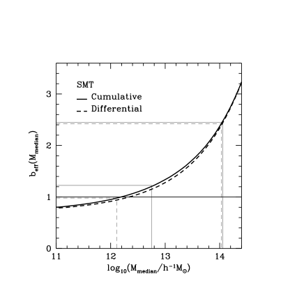
Figure 1: Theoretical predictions for the effective bias factor, $b_{\rm eff}$, of a sample of dark matter haloes, as defined by Eq. 1. The curves show the expectations for samples of haloes defined using either differential (dashed) or cumulative mass bins (solid), computed using the formalism developed by Sheth, Mo & Tormen (2001; SMT). The horizontal line indicates a bias of unity. The thin lines that intersect the curves and run parallel and perpendicular to the axes indicate the dynamic range of effective biases for the samples we use in this paper. The effective bias is computed from the GALFORM mock and the calculation is described fully in Section 2.4. The thin dashed lines show the predictions for $2$ or more members per group and the thin solid lines show the results for a minimum of $4$ members per group.

The effective bias for a sample of dark matter haloes is computed by weighting the bias factor associated with each individual halo, $b(M)$, by its abundance in the sample (e.g. Baugh et al. 1999; Padilla & Baugh 2002):

$$b_{{\rm eff}}=\frac{\int_{M_{1}}^{M_{2}}b(M)\left({\rm d}n(M)/{\rm d}M\right){\rm d}M}{\int_{M_{1}}^{M_{2}}\left({\rm d}n(M)/{\rm d}M\right){\rm d}M},$$ (1)

where ${\rm d}n(M)/{\rm d}M$ is the space density of haloes in the mass interval $M$ to $M+\delta M$. In the case of cumulative mass bins, the lower mass limit, $M_{1}$, defines the sample, as $M_{2}\rightarrow\infty$.

Fig. 1 shows the theoretical predictions for the effective bias as a function of the median mass of the sample. For differential mass samples, an interval of one decade in mass is assumed. To make these predictions, we have adopted the linear theory power spectrum used in the N-body simulation described in Section 2.2. The clustering amplitude of the overall dark matter distribution corresponds to $b=1$. The MW theory predicts that haloes with mass below a characteristic value $M_{*}$ (defined as the mass contained within a sphere for which the linear theory variance is equal to the threshold for collapse) will display a weaker clustering signal than the overall mass distribution, i.e. these haloes will have $b(M)<1$.

The dynamic range in mass of the 2PIGG samples that we consider is $\approx 10^{12}$h${}^{-1}M_{\odot}$ to $10^{14}$h${}^{-1}M_{\odot}$. Over this interval, the theoretical predictions for cumulative and differential mass bins have similar shapes, so there is no clear advantage in using differential mass bins. Moreover, the cumulative samples benefit from better statistics. For these reasons, we will subdivide the 2PIGG sample using cumulative bins in a group property related to mass (see Section 2.4).

2.4 Indicator of group mass

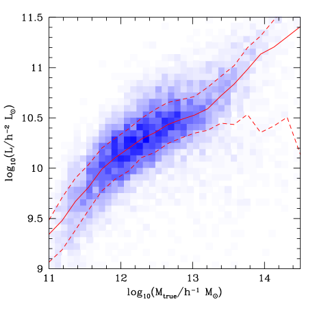
Figure 2: The corrected total group luminosity plotted as a function of true mass for groups extracted from the GALFORM mock with $z<0.12$. The grey scale indicates the number of groups, with a darker shading indicating a higher number of groups. The solid line shows the median, and the dashed lines enclose the interval within which $68\%$ of the groups lie.

Our goal in this paper is to estimate the clustering of subsamples of the 2PIGG catalogue, defined by group mass. We therefore need to find an observed property of the 2PIGGs that displays a tight correlation with the underlying or “true” group mass. Following Eke et al. (2004a), we have considered two possibilities: (i) A dynamical mass estimate that depends upon the rms radius of the group and its estimated velocity dispersion. (ii) An indirect estimate in which the corrected total group luminosity is used to infer a mass from the estimated median mass to light ratio of 2PIGGs.

From the GALFORM mock catalogue, it is possible to find the “true” mass of any group by associating it with a dark matter halo in the simulation box. The group’s “true” mass is simply the mass of the halo, as computed by summing the particles identified as members of the halo by a friends-of-friends group finding algorithm. Fig. 2 shows the relation between corrected total group luminosity and the true group mass for the GALFORM mock. The total group luminosity is obtained by summing the luminosity of the galaxies identified as members of each group, and then applying a correction to account for missing galaxies that are fainter than the apparent magnitude limit of the 2dFGRS. This correction factor is redshift dependent and reaches a factor of $\sim 2$ at $z\sim 0.12$. In Fig. 2, we only show groups with $z<0.12$. The shading represents the abundance of groups for a given total luminosity and true mass; the darker shading indicates a higher number density of groups. The solid line shows the median true mass to total luminosity relation, and the dashed lines enclose $68\%$ of the groups in each mass bin. This relation is reasonably tight over more than two decades in true mass. The equivalent comparison between the dynamical mass estimate and the true mass exhibits much more scatter (see Eke et al. 2004b). The dynamical mass estimator is a particularly poor indicator of true mass for objects less massive than $10^{13}h^{-1}M_{\odot}$. We therefore choose to employ the corrected total group luminosity as the indicator of the true group mass. However, caution is advisable when dealing with very massive groups, since, as is apparent in Fig. 2, the interval containing $68\%$ of the groups with masses $M>10^{14}h^{-1}M_{\odot}$ broadens considerably. This is due to the fact that such large groups, because of their rarity, are more likely to be found at higher redshifts, and therefore require a larger correction to be applied to the observed group luminosity to infer the total group luminosity.

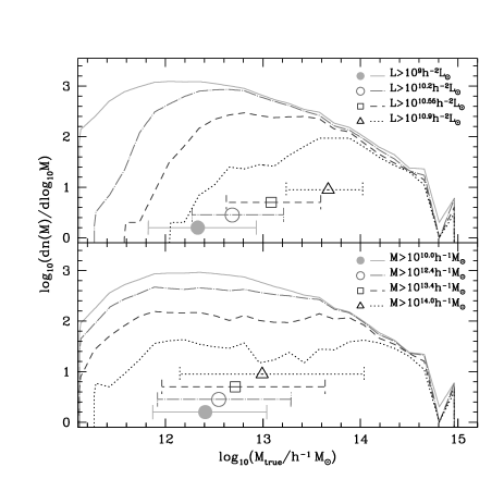
Figure 3: The distribution of true mass for subsamples of mock 2PIGG groups with at least $2$ galaxy members. The upper panel shows the mass distributions for subsamples selected by cumulative total luminosity and the lower panel shows the results for samples selected by cumulative bins in dynamical mass; the bins are given by the key in each panel. The points with error bars show the median and the 10-80 percentile range in true mass for each bin.

Further evidence supporting our choice of the total group luminosity as a mass indicator is given in Fig. 3. Here, we show the “true” mass distributions of samples from the GALFORM mock selected according to two criteria: (i) cumulative bins in total luminosity (top panel), and (ii) cumulative bins in dynamical mass (lower panel). The sample definitions are given by the key in each panel. These distributions are for groups with at least $2$ members. The different lines in each panel show the corresponding distributions of true group mass for each subsample. The points with error bars show the median and the range containing $60\%$ of the groups for the true mass distributions. It is clear from this plot that the distribution of true mass for samples selected by total group luminosity spans a larger dynamic range in mass, and the distributions have tighter percentile intervals. We have performed the same exercise for groups with a minimum of four members and reach similar conclusions. However, we note that in the case of groups with 4 or more members, there are fewer low mass groups as expected.

We now investigate how the clustering signal from group samples varies with the minimum number of group members, $n_{\rm min}$, looking at the cases where $n_{\rm min}=2$ or $4$. We compute an effective bias for each sample using Eq. 1. In Fig. 1, the effective bias is plotted at a representative mass for each sample (indicated by the lines which intersect the bias curves and run parallel and perpendicular to the mass axis). This mass is obtained using the GALFORM mocks by finding the halo mass above which the effective bias of haloes in the simulation cube matches that of the haloes recovered from the mock group catalogue. We show the effective bias for the brightest and faintest cumulative luminosity bins to illustrate the dynamic range of our clustering measurements. The dashed lines show the results of this calculation for $n_{\rm min}=2$ and the solid lines show the case where $n_{\rm min}=4$. The range of effective masses (x-axis) and clustering strengths (y-axis) probed by the different samples is widest when considering groups with $n_{\rm min}=2$.

3 Measuring the clustering of groups

We now outline the method followed to measure the clustering of the 2PIGG samples. In a sample of groups extracted from a flux limited galaxy redshift survey, the space density of groups is a function of radial distance. An accurate estimate of the radial selection function of the sample is required to make a robust measurement of the clustering of groups. The procedure that we follow to obtain the selection function from the redshift distribution of groups is set out in Section 3.1. The weighting scheme used to approximate a minimum variance estimate is given in Section 3.2, along with the estimator used to infer the correlation function.

3.1 The radial selection function

An accurate estimate of the selection function of groups in the 2PIGG samples is required to permit an analysis of the clustering signal of the groups.

The most straightforward way of doing this is to use the luminosity function of groups to obtain an estimate of the selection function which is unaffected by large scale structure. However, Eke et al. (2004c) show, using the GALFORM mock, that estimates of the group luminosity function are affected by errors in the determination of total group luminosity and by contamination, leading to systematic errors in the number density of groups of up to a factor of $4$.

The alternative is to estimate the selection function directly from the observed redshift distribution. The concern in this case is that the redshift distribution displays features that are due to large scale structure (see the histogram in Fig. 4). Care must be taken when fitting a parametric form to the observed redshift distribution to avoid ‘over-fitting’ the peaks and troughs, thereby inadvertently removing some of the clustering signal from the estimated correlation function.

With this concern in mind, we explore two procedures to describe the shape of the observed redshift distribution: fitting parametric forms or smoothing the observed redshift distribution. We will explore the influence on the measured correlation function of these different ways of fitting the redshift distribution in Section 4.1.

We adopt a fit to $N_{\rm obs}(z)$, the observed 2PIGG redshift distribution, of the form

$$N_{\rm fit}(z){\rm d}z=z^{a-1}\times\exp\left(\frac{z}{b}\right)^{a}{\rm d}z,$$ (2)

where $a$ and $b$ are parameters set by minimising the quantity

$$\chi_{N(z)}^{2}=\sum_{i=1}^{\rm nbins}\frac{(N_{\rm obs}(z_{i})-N_{\rm fit}(z_{i}))^{2}}{N_{\rm obs}^{2}(z_{i})}.$$ (3)

Alternatively, we have experimented with including a weight proportional to the volume of each redshift bin of width $\Delta z$,

$$\chi_{v,N(z)}^{2}=\sum_{i=1}^{\rm nbins}\frac{(N_{\rm obs}(z_{i})-N_{\rm fit}(z_{i}))^{2}}{N_{\rm obs}^{2}(z_{i})}z_{i}^{2}\Delta z_{i}.$$ (4)

The effect on the best fit parameter values of weighting by volume is small. From now on, best fit parameter values $a$ and $b$ obtained using Eq. 3 (and the redshift distribution constructed using them) will be referred to as unweighted fits, while those found using Eq. 4 will be referred to as volume-weighted fits. The resulting best fits for the full 2PIGG catalogues are shown in Fig. 4, as indicated by the key in the upper panel.

The parametric form adopted for the fit is particularly attractive since it can be integrated analytically to give the cumulative redshift distribution

$$\int_{0}^{z}N_{\rm fit}(z){\rm d}z\big{/}\int_{0}^{\infty}N_{\rm fit}(z){\rm d}z=1-\exp\left(\frac{z}{b}\right)^{a}.$$ (5)

The smoothed redshift distribution is obtained by smoothing the observed redshift distribution, which is tabulated in bins of width $\Delta z=0.0025$, with a top-hat window in redshift. The smoothed redshift distribution in Fig. 4 was produced by smoothing the observed distribution with a top-hat of width $\Delta z=0.01$.

Figure 4: The redshift distributions of the 2PIGG catalogue (histograms); the upper panel corresponds to the NGP region and the lower to the SGP region. The redshift distribution after smoothing is shown by the dotted line (see text for details). The dot-dashed lines show volume weighted fits (Eqs. 2 and 4), and the dashed lines show unweighted fits (Eqs. 2 and 3).

3.2 Estimating the correlation function

To obtain a minimum variance estimate of the correlation function, each group is assigned a weight given by (Efstathiou 1988):

$$w_{i}=\frac{1}{1+4\pi n(z_{i})J_{3}(s)c},$$ (6)

where we assume $J_{3}(s)=1200$h^-3Mpc³, $c$ is the angular completeness of the 2dFGRS and $n(z_{i})$ is the space density of groups at redshift $z_{i}$. In Section 4.1 we explore the impact of the choice of $J_{3}$ on the measured correlation function. The space density of groups, $n(z)$, is obtained by integrating over the product of the cosmological volume element and the adopted description of the redshift distribution; as explained above, this could be a smoothed version of the redshift distribution or a parametric fit. A catalogue of unclustered points is produced with the same radial and angular selection functions as the data. The number of random points is set to be $10$ times the number of data points, with a lower limit of $100000$. In the case of the unclustered catalogue, the weights are scaled in order to ensure that their sum matches that of the weights of the observed groups:

$$w_{R,i}=\frac{w_{R,i}}{\sum_{j}w_{R,j}}\sum_{j}w_{D,j},$$ (7)

where $R$ and $D$ indicate unclustered points and data groups respectively.

We adopt the Landy & Szalay (1993) estimator for calculating the redshift-space correlation function,

$$\xi(s)=(DD(s)-2DR(s)+RR(s))/RR(s),$$ (8)

where

$$XY(s)=\sum_{ij}w_{X,i}w_{Y,j},$$

with $X$ and $Y$ representing the actual groups ($D$) and/or points in the random catalogue ($R$); $i$ and $j$ are the indices for each individual group/random point, and $w$ corresponds to the weight defined above.

We use the same estimator to obtain the correlation function as a function of pair separation perpendicular ($\sigma$) and parallel ($\pi$) to the line-of-sight, $\xi(\sigma,\pi)$. From this correlation function, we can define the projected correlation function

$$\frac{\Xi(\sigma)}{\sigma}=\frac{2}{\sigma}\int_{0}^{\infty}\xi(\sigma,\pi)\rm{d}\sigma.$$ (9)

This quantity is free from redshift-space effects arising from peculiar motions and can be related directly to the real space correlation function (e.g. Norberg et al. 2001).

4 Testing the estimation of the correlation function

Figure 5: The accuracy with which the correlation function can be measured from the GALFORM mock catalogue for different assumptions and approximations. In each plot, the upper panel shows the systematic error on the measured correlation function, expressed as the ratio of the correlation function measured from a mock 2PIGG sample to that measured from an idealized, comparable sample. The errors on this ratio come from the rms scatter over the ensemble of Hubble Volume mocks; these are used to plot the logarithm of the relative errors in the lower panel of each plot. The different plots show how well the correlation function can be measured when the following are varied: (a) The sample definition, as given in the text: the solid lines shows results for a sample of groups brighter than a minimum luminosity, the dotted line shows a sample of groups more massive than a minimum dynamical mass limit and the dashed line shows the case of groups within a differential luminosity bin. (b) The minimum group membership. The thinner lines show results for a brighter sample of groups ($L>10^{10.9}$h^-2 L_⊙. (c) The description of the redshift distribution used to model the selection function of groups. (d) The maximum redshift used to define the catalogue; again the thinner lines show results for a brighter sample.

The measurement of the clustering of groups requires a number of choices to be made that can have an impact upon the estimated correlation function. In this section, we carry out a careful examination of our method for measuring the clustering of the mock groups, with the goal of determining a correlation function that is accurate, i.e. with minimal systematic errors, and with random measurement errors that are as small as possible. The mock catalogues described in Section 2.2 play a key role in this exercise. The GALFORM mock is used to assess systematic errors by comparing the correlation functions measured from the semi-analytic mock group catalogue with the correlation function of an equivalent sample in the simulation cube (the construction of such a catalogue is described in Section 2.2). We stress that the goal of quantifying the systematic errors is to devise a clustering measurement algorithm that minimizes these errors rather than to correct for them. The Hubble Volume mocks are used to estimate the random measurement errors, which automatically include the contribution of sample variance from large scale structure.

An important test for systematic errors in our clustering measurement is to compare the correlation function recovered from a mock group catalogue with that of a comparable, equivalent sample drawn from the distribution of groups in the simulation cube.

The rest of this section is split into two parts. In the first, we present a systematic study of how various assumptions and approximations affect the recovered correlation function. We focus attention on the size of the random measurement errors and on minimizing systematic errors in the estimated correlation function. In the second part of this section, we build on the conclusions of the first part and apply an optimal method to measure the clustering of mock 2PIGGs to determine how well we can recover trends in clustering amplitude for different subsamples of groups.

4.1 An optimal measurement of clustering

The main results of this subsection are presented in Fig. 5. Each plot in this figure is divided into two panels. The top panel in all cases compares the correlation function recovered from a GALFORM mock group catalogue with the correlation function of an equivalent sample, drawn from the simulation cube, of groups generated by GALFORM. The errors on this ratio are the rms scatter over the ensemble of 22 Hubble Volume group mocks. Note that this estimate of errors includes cosmic variance, and therefore overestimates the error bars in a comparison between results from the mock and the simulation cube, since both come from the same simulated volume. In the absence of systematic errors in the clustering measurement, this ratio would be consistent with unity, indicated by the horizontal line. The lower panel in each plot shows the logarithm of the relative error on the measured correlation function, as deduced from the rms scatter over the Hubble Volume mocks. The horizontal line indicates an error of $100\%$. To improve the clarity of the presentation, we have used a power law fit to the correlation function for separations larger than $8h^{-1}{\rm Mpc}$ in the definition of the relative error, which avoids dividing by small or negative numbers. The correlation function of the equivalent sample of groups falls below a power law on large scales, typically $s\mathrel{\hbox{\hbox to0.0pt{\hbox{\lower 4.0pt\hbox{$\sim$}}\hss}\hbox{$>$}}}15h^{-1}{\rm Mpc}$, so the plotted error is a lower limit to the true relative error on these scales. We now go through the set of choices or assumptions that needs to be made in our clustering measurement method, directing the reader to Fig. 5 where appropriate.

(i) Choice of 2dFGRS region. The differences between the correlation functions measured in the NGP and SGP regions provide a crude estimate of the errors; these differences are comparable to the errors inferred from the Hubble Volume mocks. We find that the correlation functions measured in mock NGP and SGP 2dFGRS regions are consistent within the errors. Combining the pair counts of groups in the two regions reduces the Poisson noise and sample variance in the clustering measurement. Henceforth, our results will be for combined NGP and SGP samples.

(ii) Choice of $J_{3}$ in the radial weight. The weight assigned to each group to compensate for the radial selection function requires a value for the integral of the two-point correlation function, $J_{3}(s)$ (Eq. 6). We have explored using constant values in the range $400<J_{3}/$h^-3Mpc${}^{3}<2400$, and find that the changes in the estimated correlation function are small and within the statistical errors. We adopt $J_{3}=1200$h^-3Mpc³, which corresponds to the typical asymptotic value of $J_{3}(s)$ for separations $s>10$h^-1Mpc in the Hubble Volume mocks.

(iii) Sample definition. Fig. 5(a) compares the correlation function measured for samples defined in different ways: by setting (i) a lower limit on total group luminosity, $L>10^{10.2}$h${}^{-2}L_{\odot}$ (solid line), (ii) a lower limit on dynamical mass, $M_{\rm dyn}>10^{12.4}h^{-1}M_{\odot}$ (dotted line), which, for the median mass-to-light ratio of the 2PIGGs (Eke et al. 2004b), corresponds to the luminosity cut in (i), and (iii) a differential luminosity sample defined by $10^{10.25}<L/$h${}^{-2}L_{\odot}<10^{10.55}$ (dashed line). The correlation function measured for the sample of groups brighter than the luminosity threshold in (i) has the smallest systematic and random errors. This adds further weight to the preference arrived at for cumulative bins in luminosity in Section 2.4. The three remaining panels, Fig. 5(b),(c) and (d) show the errors on $\xi(s)$ for samples of mock groups with $L>10^{10.2}$h${}^{-2}L_{\odot}$ (shown by solid lines), and, in some cases for a brighter sample with $L>10^{10.9}h^{-1}M_{\odot}$ (indicated by dashed lines).

(iv) Minimum number of group members. We compare the accuracy of the correlation function for groups with a minimum number of members of $n_{\rm min}=2$ (solid lines) and $n_{\rm min}=4$ (dashed lines) in Fig. 5(b). The systematic errors on the correlation functions recovered from the mocks are roughly comparable in the two cases. The random errors, however, are smaller for the case of $n_{\rm min}=2$. This is expected since this sample contains more groups. We recall that samples of groups with $n_{\rm min}=2$ span a wider range in mass (see Fig 3 in Section 2.4). The dashed lines in Fig. 5(b) show the results for a brighter sample of groups, as explained at the end of (iii) above. This sample contains fewer groups and so the random errors are somewhat larger than before, particularly at small separations. The systematic errors in the correlation function recovered from the mock 2PIGG also become significant below $s\approx 2h^{-1}$Mpc for the brighter sample.

Figure 6: The relative errors on our measurement of $\xi(s)$, obtained by dividing the rms scatter in $\xi(s)$ from the Hubble Volume mocks by the mean value of $\xi(s)$ for $s<8$h^-1Mpc, and a fit to the mean $\xi(s)$ (over $8<s/($h^-1Mpc$)<15$) for $s>8$h^-1Mpc. The horizontal black line shows the $100\%$ error limit. Different line types correspond to different subsamples as indicated by the key.

(v) Selection function model. The impact on the correlation function of using different approximations to the form of the redshift distribution of groups to model their selection function is shown in Fig. 5(c). The solid line shows how well the correlation function can be measured using a parametric fit to the redshift distribution of groups in the mock, as described in Section 3.1; the dotted line shows the results when a volume weighting is applied to determine the best fit parameters. On small scales, $s<3h^{-1}$Mpc, the systematic and random errors are very similar in these two cases. On larger scales however, the unweighted fit results in a more faithful and less noisy measurement of the correlation function. The evidence in this panel shows that the approach of using the smoothed redshift distribution of groups to model their selection function (dashed line) is clearly flawed, leading to a significantly discrepant estimate of the correlation function for separations $s>1h^{-1}$Mpc.

Figure 7: The correlation functions measured in the GALFORM 2PIGG mock for samples defined by lower group luminosity limits (symbols with error bars). In the left hand column, results are shown for $n_{\rm min}=2$ and in the right for $n_{\rm min}=4$. These measurements are compared with the correlation functions of equivalent samples of groups taken from the simulation cube (lines). Two different methods of constructing these equivalent samples have been used. In the top row, the equivalent samples have the same mass function as the groups in the sample from the mock 2PIGG catalogue. In the bottom row, the equivalent samples are complete above some halo mass, chosen so that the groups have the same effective bias as those recovered from the mock 2PIGG catalogue.

(vi) Sample redshift limit. An increase in the redshift limit of the sample leads to a larger volume and the associated increase in the size of the sample. However, these additional groups come at the expense of requiring a larger correction to the observed group luminosity to deduce the total group luminosity. The consequences of varying the maximum redshift limit of the sample are presented in Fig. 5(d), where the cases $z_{\rm max}=0.12$ (light lines) and $z_{\rm max}=0.15$ (dark lines) are considered. There is a negligible difference in the random measurement errors for these redshift limits. The correlation function is more accurately recovered for $z_{\rm max}=0.12$.

The conclusions of this subsection are that an optimal measurement of the clustering of the 2PIGG catalogue will be obtained under the following conditions: (i) The pair counts in the NGP and SGP regions of the 2dFGRS are combined. (ii) The value of $J_{3}$ is taken to be $1200$h^-3Mpc³, though the results are fairly insensitive to the exact value. (iii) Cumulative bins in luminosity are used to define subsamples of groups from the 2PIGG catalogue. (iv) $n_{\rm min}=2$ is used, which leads to the most reliable measurements. (v) The most accurate model of the selection function is obtained by a simple parametric fit to the observed group redshift distribution. (vi) A conservative redshift of $z_{\rm max}=0.12$ is used.

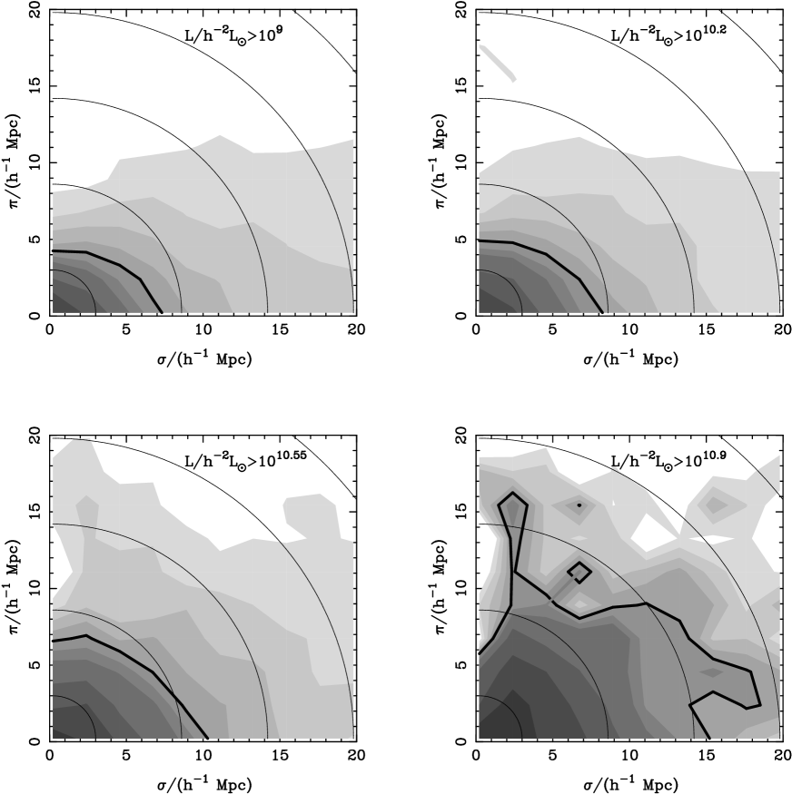
Figure 8: The correlation function, $\xi(\sigma,\pi)$, for selected 2PIGG samples, as indicated by the label on each panel. The grey scale indicates the amplitude of the correlation function, with darker shading indicating stronger clustering: $\xi(\sigma,\pi)=0.2,0.4,0.6,0.8,1,1.2,1.4,2,3$ and $5$ are shown. The $\xi=1$ contour is also marked by a thick black line. The thin black lines show the expected shape of the $\xi(\sigma,\pi)$ contours in the absence of redshift space distortions of the clustering pattern.

4.2 The clustering of subsamples of groups

We now investigate how well we can distinguish between the clustering signals displayed by different samples of groups defined by mass. We also test our clustering measurement algorithm to see how faithfully the clustering signal can reproduce an idealized measurement. This is an important consideration, as this determines the strength of the constraints we can place on theoretical models of the clustering of galactic systems.

The errors on the measured correlation function are obtained from the rms scatter over the ensemble of Hubble Volume mock 2PIGG catalogues. We show these relative errors in Fig. 6. The horizontal line marks an error of $100\%$. This plot indicates that we should be able to get a robust measurement of the correlation function out to pair separations of $s\sim 30h^{-1}$Mpc. The small scale limit depends more upon the sample under consideration, due to the changing space density of groups. For the full group sample, the correlation function can be measured down to separations below $s\sim 1h^{-1}$Mpc; for the most luminous sample, which has a much lower space density, the smallest pair separation that can be probed is $s\approx 3h^{-1}$Mpc.

To test the accuracy of our clustering measurements, we have extracted samples of groups from the GALFORM mock catalogue defined by a series of lower limits in total group luminosity as discussed earlier. The clustering measured for these samples is compared with that of samples drawn from the simulation cube using two different criteria to construct equivalent samples as discussed earlier. The samples drawn from the simulation cube are idealized in the sense that they do not have a radial or angular selection function imposed upon them as is the case for the mock 2PIGG catalogue. Moreover, the groups occupy dark matter haloes identified by a friends-of-friends group finder. The mass of a group in the simulation cube is known very accurately: it is simply the sum of the mass of the dark matter particles connected by the group finder.

The correlation functions measured for mock group subsamples defined by a lower limit on total group luminosity are compared with the results for the equivalent samples drawn from the simulation cube in Fig. 7. The top row of this figure shows the comparison when the equivalent samples are set up to reproduce the mass function of groups recovered from the mock group catalogue for each luminosity subsample. The bottom row shows the comparison for equivalent samples constructed to match the effective bias estimated from the mock subsamples. The left hand column shows the results for groups with a minimum membership $n_{\rm min}=2$, and the right hand column for $n_{\rm min}=4$. The clustering measurements from the mock subsamples are in impressively good agreement with the results obtained for the equivalent samples in the simulation cube, particularly for the case of $n_{\rm min}=2$. The equivalent samples constructed to reproduce the effective bias of mock group subsamples are in somewhat better agreement with the measurements from the mocks for the brighter group samples.

The agreement in clustering amplitude between samples of groups taken from a mock and those extracted from an idealized simulation is significant; it means that we fully understand the impact of making a mock group catalogue on the measurement of the clustering of groups and can use the clustering of 2PIGG samples to constrain theoretical models of structure formation.

Figure 9: The projected correlation function of selected 2PIGG samples. The samples are indicated by the key; error bars are plotted on the measurements for selected samples for clarity. The solid line shows a fit to the projected correlation function of 2dFGRS galaxies taken from Hawkins et al. (2003).

5 2PIGG results

Figure 10: Left panel: The redshift space correlation function, $\xi(s)$, measured for samples of 2PIGGs. The samples are shown by the key. Error bars are plotted for selected samples for clarity. The solid line shows $\xi(s)$ for 2dFGRS galaxies, measured by Hawkins et al. (2003). Right panel: The ratio of the group correlation function to the galaxy correlation function, plotted on a logarithmic scale.

In this section we measure the clustering amplitude of the real 2PIGGs for samples defined by total group luminosity. Some basic properties of the samples are given in Table 1. We apply the optimal clustering measurement algorithm set out at the end of Section 4.1. We combine the pair counts in these regions to estimate the correlation function. We have checked that the measurements for the individual regions agree within the errors.

An important test of the integrity of a group catalogue is the form of the correlation function measured in bins of pair separation parallel ($\pi$) and perpendicular ($\sigma$) to the line of sight, $\xi(\sigma,\pi)$. Padilla & Lambas (2003a,b) explored different techniques used in the construction of group and cluster catalogues. They found that the shape of $\xi(\sigma,\pi)$ is a powerful way to reveal spurious agglomerations of galaxies. A tell-tale sign of problems with the composition of galaxy groups is a significant enhancement of the correlation function, $\xi(\sigma,\pi)$, in the $\pi$ direction, as seen in the early analyses of Abell catalogue clusters (e.g. Bahcall & Soneira 1983; Sutherland 1988). Such a distortion of the clustering pattern is seen for 2dFGRS galaxies, due to the large peculiar motions inside massive virialised structures (Peacock et al. 2001; Hawkins et al. 2003). However, for the case of groups and clusters, such virialised structures are not predicted in viable models of structure formation (Kaiser 1987; Padilla et al. 2001; Padilla & Baugh 2002). The correlation function, $\xi(\sigma,\pi)$, for samples of 2PIGGs is shown in Fig. 8. There is no enhancement of the clustering signal in the $\pi$ direction. The contours of constant clustering amplitude are, however, affected by peculiar motions, showing the flattening due to the infall motions expected in the gravitational instability paradigm (Padilla et al. 2001; Peacock et al. 2001). There is also a clear increase in clustering amplitude with sample luminosity.

The projected correlation function, $\Xi(\sigma)/\sigma$, is the integral of $\xi(\sigma,\pi)$ over the $\pi$ direction (e.g. Norberg et al. 2001). This statistic is unaffected by peculiar motions. In Fig. 9, we show the projected correlation functions for selected samples of 2PIGGs. The black line shows the best fit to the projected correlation function of galaxies in the 2dFGRS for comparison (Hawkins et al. 2003). We find that the lowest luminosity sample plotted is less strongly clustered than the galaxy distribution, a point to which we return later on in this section. The brightest sample of groups displays a clustering amplitude that is an order of magnitude stronger than that measured for 2dFGRS galaxies.

The projected correlation function, due to the way it is calculated, can be unreliable if the correlation function is noisy on large scales. A more robust quantity in such cases is the redshift space correlation function, $\xi(s)$. This quantity is the average of $\xi(\sigma,\pi)$ within annuli centred on $s=\left(\sigma^{2}+\pi^{2}\right)^{1/2}$. The redshift space correlation function measured for 2PIGG samples with membership $n_{\rm min}\geq 2$ is plotted in the left-hand panel of Fig. 10. For reference, we also plot the redshift space correlation function of 2dFGRS galaxies measured by Hawkins et al. (2003). The correlation function of the group samples has a similar shape to that obtained for galaxies, on scales where a comparison is reliable. There is, however, a dramatic change in clustering amplitude with group luminosity, mirroring that seen for the projected correlation function in Fig. 9. These points are emphasized in the right hand panel of Fig. 10, in which we plot the group correlation function divided by the galaxy correlation function. There is a relative bias between the spatial distribution of groups and galaxies. For the full 2PIGG sample, and also for the next faintest luminosity sample, this relative bias is actually an anti-bias; these groups are more weakly clustered than the galaxies. The brightest groups, on the other hand, are almost ten times more strongly clustered than the galaxy distribution.

A useful summary of the clustering measurements can be made by plotting the correlation length, $s_{0}$, as a function of the mean group separation, $d_{c}$, which is related to the space density of groups, $n$, by $d_{c}=1/n^{1/3}$. The space density of groups is estimated using the cumulative $b_{\rm J}-$band luminosity function of 2PIGGs out to $z=0.12$ (Eke et al. 2004b). The space density of each subsample is simply the luminosity function evaluated at the appropriate lower limit in luminosity. We estimate the correlation length (defined by $\xi(s_{0})=1$) by fitting a power law to the measured redshift space correlation function for pair separations in the range $0.4<\log_{10}(s/$h^-1Mpc$)<1.3$. Our results are fairly insensitive to perturbations to this range.

The clustering strength of 2PIGG samples versus mean group separation is plotted in Fig. 11. There is an increase in clustering strength with the mean separation of groups in each sample; the clustering strength increases slightly less rapidly than the change in group separation. There is very good agreement between the results for $n_{\rm min}=2$ and $n_{\rm min}=4$ for group separations for which a comparison is possible. Fig. 11 also shows the $s_{0}$-$d_{c}$ relation in the GALFORM mock 2PIGG catalogue with $n_{min}=2$, which is in very close agreement with the results from the real 2PIGG samples. The solid and dotted lines show the measurements for equivalent samples of groups drawn from the simulation cube. The solid line gives the $s_{0}$-$d_{c}$ relation in redshift space and the dotted line shows the real space results. The clustering amplitude is typically $10\%$-$20\%$ weaker in real space than in redshift space.

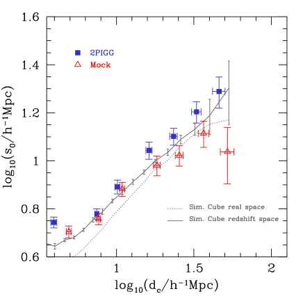
Figure 11: The correlation length in redshift space, $s_{0}$, plotted as a function of the mean group separation, $d_{c}$. The 2PIGG results are shown by filled squares for $n_{\rm min}=2$. Also shown for comparison are measurements from the GALFORM mock plotted with triangles. The solid line shows the $s_{0}-d_{c}$ relation obtained from the simulation cube for equivalent samples of groups (see text). The dotted line shows how these results change when the correlation length is measured in real space.

Figure 12: A comparison of the $s_{0}-d_{c}$ relation for different samples. The squares show the results from the 2PIGGs for $n_{\rm min}=2$. The other symbols show a selection of data taken from the literature, as indicated by the key. The lines show fits to subsets of the data, with sources indicated by the key.

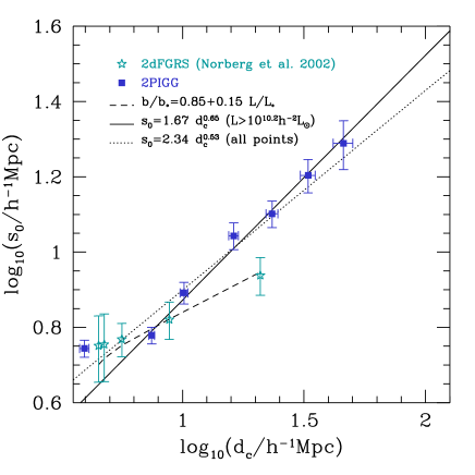
Figure 13: A comparison of the $s_{0}-d_{c}$ relation for 2PIGG groups (squares) and for 2dFGRS galaxies (stars, taken from Norberg et al. 2002a). The solid line is a fit to the 2PIGG clustering data, excluding the lowest luminosity sample; the dotted line is a fit to the 2PIGG results including the faintest sample. The dashed line shows the fit to the clustering strength-luminosity relation fitted to 2dFGRS data by Norberg et al. (2001).

The 2PIGG results are compared with a selection of measurements taken from the literature in Fig. 12. This comparison between datasets should be treated with caution due to a number of differences in the way the various samples have been defined and analysed: namely, in decreasing order of seriousness: (i) the technique used to identify groups and clusters, (ii) the derivation of a value for the mean inter-group separation and (iii) the calculation of the correlation length.

Zandivarez et al. (2003) measured the clustering of groups in a catalogue constructed from the 100k release of 2dFGRS data by Merchán & Zandivarez (2002). The two most abundant samples of groups analysed by Zandivarez et al. have a significantly higher clustering amplitude than we recover for 2PIGG groups of comparable abundance. Zandivarez et al. estimated $d_{c}$ from a dynamical estimate of the group mass which they translated into a spatial abundance using the measured mass function of groups (Martínez et al. 2002). Moreover, Zandivarez et al. only consider groups with $n_{\rm min}=4$; such groups are probably only associated with low mass systems through errors in the dynamical mass estimates. The abundance of groups in the Updated Zwicky Catalogue was estimated in a similar way by Merchán et al. (2000). Bahcall et al. (2003) have applied a photometric technique (Annis et al. 2004) to a subset of the Sloan survey data to obtain a sample of clusters that overlaps with the most luminous 2PIGG groups and with APM Survey clusters (Croft et al. 1997; Dalton et al. 1997). The Sloan measurements are in reasonable agreement with the results from APM clusters and are marginally lower than the 2PIGG values at comparable abundances. However, both the SDSS and APM clusters are identified in projection. The trend of clustering strength versus abundance found for 2PIGGs agrees quite well with the measurements from X-ray selected cluster samples (Abadi, Muriel & Lambas 1998; Collins et al. 2000; Lee & Park 2002).

The dotted line in Fig. 12 shows the $s_{0}$-$d_{c}$ relation advocated by Bahcall & West (1992), whereas the dot-dashed line is the relation proposed by Bahcall et al. (2003); the dashed line is the fit of Zandivarez et al. (2003) to their data. The analogous fit to the 2PIGG results is plotted in Fig. 13 for clarity. If the faintest groups are ignored, the 2PIGG results are described by the relation $s_{0}=1.67d_{c}^{0.65}$. This is somewhat steeper than the fit of Bahcall et al. (2003).

We compare the clustering of 2PIGG groups with 2dFGRS galaxies in Fig. 13. The clustering amplitude of 2dFGRS galaxies is taken from Norberg et al. (2002a), who analysed volume limited samples defined by galaxy luminosity. The curve plotted over the galaxy clustering measurements shows the predictions of the simple relation between relative clustering strength and luminosity deduced by Norberg et al. (2001). The full sample of 2PIGGs is more weakly clustered than $L_{*}$ and brighter galaxies. On the other hand, the trend of clustering strength with pair separation is stronger for groups than it is for galaxies.

6 Conclusions

We have measured the clustering of groups in the 2PIGG sample constructed from the 2dFGRS by Eke et al. (2004a). The group catalogue, made up of galactic systems with a minimum of two members, contains $\sim$29,000 groups, out of which $\sim$16,000 are at $z<0.12$. The sample is sufficiently large and homogenous that a robust measurement of clustering is possible for subsamples of groups defined by their corrected total luminosity. Our analysis has relied extensively on the use of various mock group catalogues constructed using high resolution N-body simulations populated with galaxies using the GALFORM semi-analytic model (Cole et al. 2000; Benson et al. 2000, 2003).

In summary, the main conclusions we have reached are the following:

1. The main goals of this paper were to make a robust measurement of the clustering of galaxy groups with the aim of exploring the dependence of the clustering amplitude on a property related to group mass (for example the total group luminosity) and to compare the results with theoretical predictions. We have tested our algorithm for estimating the correlation function by comparing results obtained from a mock 2PIGG catalogue with those derived from equivalent samples drawn from the N-body simulation cube. The success of this comparison is significant for two reasons. Firstly, in order to make a robust measurement of the clustering of groups from a flux limited galaxy survey, it is necessary to make a number of approximations and to choose certain parameter values (see Section 4.1). We have tuned the algorithm for measuring the clustering of 2PIGG groups by requiring a close match between the correlation functions estimated from the mocks and the original results from the simulation cube. Secondly, the ability to extract equivalent samples of groups from a simulation volume with the same clustering as samples taken from mock 2PIGG catalogues makes it possible to interpret the 2PIGG clustering results in the context of structure formation models.

2. We find that clustering amplitude increases substantially with total group luminosity. The 2PIGG catalogue allows clustering measurements to be made for samples spanning a factor of $25$ in median total luminosity. The correlation function increases in amplitude by an order of magnitude over this luminosity interval. Another way of expressing this is that the redshift space correlation length changes by a factor $\approx 3.5$ from the faintest to the brightest sample. The most luminous groups we consider have a mean pair separation that is $\approx 5.5$ times greater than that of the full group sample. There is little change in the shape of the correlation function with group luminosity.

3. The shape of the redshift space correlation function of groups is very similar to that measured for 2dFGRS galaxies on the scales for which a comparison is possible. The full 2PIGG sample has a weaker clustering amplitude than is measured for 2dFGRS galaxies; the correlation length of the 2PIGG sample with $n_{\rm min}=2$ is $s_{0}=5.5\pm 0.1h^{-1}$Mpc, whilst that of 2dFGRS galaxies is $6.82\pm 0.28h^{-1}$Mpc (Hawkins et al. 2003). However, the clustering amplitude of brighter samples of groups is much greater than that of 2dFGRS galaxies.

4. The correlation functions measured for 2PIGG samples are in very good agreement with the predictions of a semi-analytic model of galaxy formation, the GALFORM model (Cole et al. 2000; Benson et al. 2003), in a cold dark matter universe with a cosmological constant ($\Lambda$CDM). Previous work has compared the predictions of the $\Lambda$CDM model with measurements of the correlation length versus abundance relation for rich clusters (Governato et al. 1999; Colberg et al. 2000). To extend the theoretical calculations down to group-sized systems, it is essential to extend the predictions of the spatial distribution of dark matter haloes in the $\Lambda$CDM cosmology with a model for galaxy formation. The galaxy formation model predicts how the dark matter haloes should be populated with galaxies. For this reason, the clustering of groups provides a more stringent test of theories of galaxies formation than the clustering of the richest clusters.

5. The trend of correlation length (measured in redshift space) against mean inter-group separation can be quantified as: $s_{0}=1.67d_{c}^{0.65}$. The 2PIGG catalogue has made possible a robust measurement of the clustering of galactic systems, ranging from poor groups to rich clusters, from one sample for the first time. Our results are in general agreement with those obtained previously for rich groups and clusters.

Galaxies and groups of galaxies trace the underlying distribution of dark matter haloes in different ways. Galaxies trace the halo distribution in a complex way. The halo occupation distribution (HOD), which depends strongly on halo mass, has been used extensively to constrain theoretical models (e.g. Benson et al. 2000; Peacock & Smith 2000; Seljak 2000; Berlind et al. 2003). In principle, the group sample should trace the halo distribution in a simple fashion, with every halo above some mass spawning one galaxy group. However, in practice, the identification of groups in real surveys is complicated, making this ideal difficult to attain. Because of this it is essential to devise a scheme to quantify the fidelity of a group catalogue and to uncover any biases in comparisons with theoretical models by applying the group finder to mock catalogues (Eke et al. 2004a).

The difference between the clustering amplitude measured for the full 2PIGG and the full 2dFGRS galaxy samples can be readily understood in terms of the HOD. Ideally, the groups have a one-to-one correspondence with the underlying dark matter haloes within some mass interval. The galaxies obviously sample haloes in the same mass range, but with a weight that increases with halo mass, since the most massive haloes host more than one galaxy. Thus, the more massive haloes, which are the more strongly clustered, make a larger contribution to the correlation function of 2dFGRS galaxies than they do in the case of the full 2PIGG sample. The clustering of galaxy groups as a function of group luminosity therefore provides an important new test of theories of galaxy formation.

References

- [] Abadi M.G., Lambas D.G., Muriel H., 1998, ApJ, 507, 526.
- [] Annis J., et al., 2004, in preparation
- [] Bahcall N.A., Soneira R.M., 1983, ApJ, 270, 20.
- [] Bahcall N.A., West M.J., 1992, ApJ, 392, 419.
- [] Bahcall N.A., Dong F., Hao L., Bode P., Annis J., Gunn J. E., Schneider D. P., 2003, ApJ, 599, 814.
- [] Baugh C. M., Benson A.J., Cole S., Frenk C.S., Lacey C.G., 1999, MNRAS, 305, L21.
- [] Benson A.J., Cole S., Frenk C.S., Baugh C.M., Lacey C.G., 2000, MNRAS, 311, 793.
- [] Benson A.J., Lacey C.G., Baugh C.M., Cole S., Frenk C.S., 2002, MNRAS, 333, 156.
- [] Benson A.J., Bower R.G., Frenk C.S., Lacey C.G., Baugh C.M., Cole S., 2003, ApJ, 599, 38.
- [] Berlind A.A., Weinberg D.H., Benson A.J., Baugh C.M., Cole S., Davé R., Frenk C.S., Jenkins A., Katz N., Lacey C.G., 2003, ApJ, 593, 1.
- [] Colberg J. M., et al., 2000, MNRAS, 319, 209.
- [] Cole S., Kaiser N., 1989, MNRAS, 237, 1127.
- [] Cole S., Hatton S., Weinberg D.H., Frenk C.S., 1998, MNRAS, 300, 945.
- [] Cole S., Lacey C.G., Baugh C.M., Frenk C.S., 2000, MNRAS, 319, 168.
- [Colless et al.(2001)] Colless M. et al. (the 2dFGRS team), 2001, MNRAS, 328, 1039
- [Colless et al.(2003)] Colless M. et al. (the 2dFGRS team), 2003, astro-ph/0306581
- [] Collins C. A., et al., 2000, MNRAS, 319, 939.
- [] Croft R.A.C., Dalton G.B., Efstathiou G., Sutherland W.J., Maddox S.J., 1997, MNRAS, 291, 305.
- [] Dalton G.B., Maddox S.J., Sutherland W.J., Efstathiou G., 1997, MNRAS, 289, 263.
- [] Davis M., Efstathiou G., Frenk C.S., White S.D.M., 1985, ApJ, 292, 371.
- [] Efstathiou G., 1988, in Comets to cosmology, ed A. Lawrence, Proc 3rd IRAS Conference, Springer-Verlag, Berlin.
- [] Eke V.R. et al. (the 2dFGRS Team), 2004a, MNRAS, 348, 866. (astro-ph/0402567).
- [] Eke V.R. et al. (the 2dFGRS Team), 2004b, MNRAS, submitted, astro-ph/0402566.
- [] Eke V.R. et al. (the 2dFGRS Team), 2004c, in preparation.
- [] Evrard, A.E., MacFarland, T.J., Couchman, H.M.P., Colberg, J.M., Yoshida, N., White, S.D.M., Jenkins, A., Frenk, C.S., Pearce, F.R., Peacock, J.A., Thomas, P.A., 2002, ApJ, 573, 7.
- [] Geller M.J., Huchra J.P., 1983, ApJS, 52, 61.
- [] Girardi M., Boschin W., da Costa L.N., 2000, A&A, 353, 57.
- [] Governato F., Babul A., Quinn T., Tozzi P., Baugh C.M., Katz N., Lake G., 1999, MNRAS, 307, 949.
- [] Hawkins E., et al. (the 2dFGRS Team), 2003, MNRAS, 346, 78.
- [] Helly, J.C., Cole, S., Frenk, C.S., Baugh, C.M., Benson, A., Lacey, C., 2003, MNRAS, 338, 903.
- [] Jenkins A., Frenk C.S., White S.D.M., Colberg J.M., Cole S., Evrard A.E., Couchman H.M.P., Yoshida N., 2001, MNRAS, 321, 372.
- [] Jing Y., Zhang, J., 1988, A&A, 190, L21.
- [] Kaiser N., 1987, MNRAS, 227, 1.
- [] Kashlinsky A., 1987, ApJ, 317, 19.
- [] Kauffmann G., Colberg J.M., Diaferio A., White S.D.M., 1999, MNRAS, 303, 188.
- [] Landy S.D., Szalay A.S., 1993, ApJ, 412, 64.
- [] Lee S., Park C., 2002, J. Korean Astron. Soc., 35, 111.
- [] Maia M.A.G., da Costa L.N., 1990, ApJ, 352, 457.
- [] Martínez H.J., Zandivarez A., Merchán M.E., Domínguez M.J.L., 2002, MNRAS, 337, 1441.
- [] Merchán M.E., Maia M.A.G., Lambas D.G., 2000, ApJ, 545, 26.
- [] Merchán M., Zandivarez A., 2002, MNRAS, 335, 216.
- [] Mo H.J., White S.D.M., 1996, MNRAS, 282, 347.
- [] Norberg P., et al., (the 2dFGRS Team), 2001, MNRAS, 328, 64.
- [] Norberg P., et al., (the 2dFGRS Team), 2002a, MNRAS, 332, 827.
- [] Norberg P., et al., (the 2dFGRS Team), 2002b, MNRAS, 336, 907.
- [] Padilla N.D., Merchán M.E., Valotto C.A., Lambas D.G., Maia M.A.G., 2001, ApJ, 554, 873.
- [] Padilla N.D., Baugh C.M., 2002, MNRAS, 329, 431.
- [] Padilla N.D., Lambas D.G., 2003a, MNRAS, 342, 519.
- [] Padilla N.D., Lambas D.G., 2003b, MNRAS, 342, 532.
- [] Peacock J.A., Smith R.E., 2000, MNRAS, 318, 1144.
- [] Peacock J.A., et al. (the 2dFGRS Team), 2001, Nature, 410, 169.
- [] Press W.H., Schechter P., 1974, ApJ, 187, 425.
- [] Ramella M., Geller M.J., Huchra J.P., 1990, ApJ, 353, 51.
- [] Seljak U., 2000, MNRAS, 318, 203.
- [] Sheth R.K., Mo H.J., Tormen, G., 2001, MNRAS, 323, 1.
- [] Spergel D.N., et al. (the WMAP Team), 2003, ApJS, 148, 175.
- [] Sutherland W., 1988, MNRAS, 234, 159.
- [] Zandivarez A., Merchán M.E., Padilla N.D., 2003, MNRAS, 344, 247.