The Luminosity Function and Color-Magnitude Diagram of the Globular Cluster M12

Abstract

In this paper we present the $V$ and $I$ luminosity functions and color-magnitude diagrams derived from wide-field ($23\arcmin\times 23\arcmin$) $BVI$ photometry of the intermediate metallicity ([Fe/H]$\sim-1.3$) Galactic globular cluster M12. Using observed values (and ranges of values) for the cluster metallicity, reddening, distance modulus, and age we compare these data to recent $\alpha$-enhanced stellar evolution models for low mass metal-poor stars. We describe several methods of making comparisons between theoretical and observed luminosity functions in order to isolate the evolutionary timescale information the luminosity functions contain. We find no significant evidence of excesses of stars on the red giant branch, although the morphology of the subgiant branch in the observed luminosity function does not match theoretical predictions in a satisfactory way. Current uncertainties in $T_{\mbox{eff}}$-color transformations (and possibly also in other physics inputs to the models) make more detailed conclusions about the subgiant branch morphology impossible. Given the recent constraints on cluster ages from the WMAP experiment (Spergel et al. 2003), we find that good fitting models that do not include He diffusion (both color-magnitude diagrams and luminosity functions) are too old (by $\sim 1-2$ Gyr) to adequately represent the cluster luminosity function. The inclusion of helium diffusion in the models provides an age reduction (compared to non-diffusive models) that is consistent with the age of the universe being $13.7\pm 0.2$ Gyr (Bennett et al. 2003).

1 Introduction

One of the observational tools available for the study of low-mass ($\sim 0.5-1~{}M_{\odot}$), metal-poor stars is the luminosity function (LF) of Galactic globular clusters (GGCs). A GGC usually presents a large, chemically homogeneous, and coeval stellar population — samples of a kind that cannot easily be extracted from halo field stars. In particular, the LF counts of evolved stars (from the main-sequence turnoff to the tip of the red giant branch) are directly related to the rate of nuclear fuel consumption (Renzini & Fusi Pecci, 1988). Thus, a high-precision LF indirectly reflects interior stellar physics, and thus can complement observations of stellar surface conditions.

Previous LF studies of GGCs have given hints that non-standard physics might be required in the models. First, in the case of several metal-poor clusters an excess of stars on the sub-giant branch (SGB) has been noted. In a study that combined the LFs of M68, NGC 6397, and M92, Stetson (1991) found an excess located just brighter than the main-sequence turnoff (MSTO). A similar excess was also observed in M30 by Bolte (1994) and confirmed by Bergbusch (1996), Guhathakurta et al. (1998), and Sandquist et al. (1999). Such an excess could be the result of enhanced energy transport in the cores of main-sequence (MS) stars nearing hydrogen exhaustion (e.g. Faulkner & Swenson 1993). To date excesses have only been seen in extremely metal-poor clusters and at low statistical significance; the LFs of M5 (Sandquist et al., 1996) and M3 (Rood et al., 1999) did not reveal such excesses. Second, studies by Stetson (1991), Bergbusch & VandenBerg (1992), Bolte (1994), Bergbusch (1996), and Sandquist et al. (1999) have shown that there may exist an over-abundance of red giant branch (RGB) stars relative to the number of MS stars in some clusters. This may be indicative of physical processes such as core rotation (Vandenberg, Larson, & de Propris, 1998) and/or deep mixing (Langer, Bolte, & Sandquist, 2000). The observed LFs of other GGCs, however, have been argued to agree with theory (degl’Innocenti, Weiss, & Leone, 1997; Zoccali & Piotto, 2000; Rood et al., 1999). While the LF of M3 derived by Rood et al. (1999) is one of the largest to date, the study by Zoccali & Piotto (2000) has a smaller overall statistical significance due to the smaller overall star samples. In general, only thorough studies of large star populations in GGCs will help confirm or deny the reality of these kinds of excesses.

A physical effect that is becoming part of standard stellar models is the gravitational settling of heavy elements (Richard et al., 2002). Solar models show (Proffitt, 1994; Richard et al., 1996; Bahcall et al., 1997; Guenther & Demarque, 1997) that helioseismic data and the inferred radius of the convection zone (Christensen-Dalsgaard, Gough, & Thompson, 1992) can only be matched by theory if the surface abundance of helium has decreased with time. Stellar evolution models for low mass, metal-poor stars that include the effects of He diffusion have been previously constructed (Proffitt & Vandenberg, 1991; Chaboyer et al., 1992; Straniero, Chieffi, & Limongi, 1997; Chaboyer et al., 2001) to investigate the observational effects on GGC LFs and color-magnitude diagrams (CMDs). One important result of these studies was that by adding He to the core of the stars, and consequently displacing H, the duration of the MS lifetime is shortened. This results in a lower MSTO luminosity for a given age and has strong implications for the derivation of GGC ages (Chaboyer et al., 1992; VandenBerg et al., 2002). Using these diffusive models GGC ages may be reduced as much as $10-15$% ($\sim 1-2$ Gyr) compared to models that do not incorporate diffusion (Straniero, Chieffi, & Limongi, 1997; VandenBerg et al., 2002), although the reduction could be as little as $4-7$% ($\sim 0.5-1$ Gyr) depending on the presence of complete or partial ionization in the models (Richard et al., 2002; Gratton et al., 2003). Given the recent analysis of the WMAP data from the cosmic background radiation, we now have a tight cosmological upper-limit on the age of the universe of $13.7\pm 0.2$ Gyr (Bennett et al., 2003; Spergel et al., 2003). As a consequence, theoretical stellar evolution models that do not include diffusion (at least for He) may produce globular cluster isochrones that are too old.

In this paper we present $BVI$ photometric data derived from wide-field CCD photometry of the GGC M12 (NGC 6218, C 1644-018). This bright, large, intermediate metallicity ([Fe/H]$\sim 1.3$) cluster should provide an interesting comparison to other well-studied intermediate clusters such as M3 and M5. M12 is also an extreme “second parameter” cluster [$(B-R)/(B+V+R)=0.92$; Lee, Demarque, & Zinn (1994)]. Ground-based photometric data on M12 have most recently been presented by von Braun et al. (2002; hereafter VB02), Rosenberg et al. (2000; hereafter R00), and Brocato et al. (1996; hereafter B96). Space-based data on M12 was published by Piotto et al. (2002) as part of a HST GGC snapshot survey. Sato, Richer, & Fahlman (1989; hereafter S89) presented a deep CMD and LF for the inner regions of M12, but to date no LF of the evolved stellar populations of M12 has been determined.

In this study we focus on comparing our data (in the form of LFs and CMDs) to three sets of stellar evolution models. In $\S 2$ we discuss the observations, data reduction and photometry, photometric calibration, and comparisons to existing photometry. In $\S 3$, we present the photometry in the form of CMDs and derived fiducial lines. $\S 4$ discusses the cluster reddening, distance modulus, age, and metallicity which are the necessary input parameters to the comparison of the theoretical LF with the observed. The computation of the observed LF and incompleteness corrections are discussed in $\S 5$. In $\S 6$ we compare the data to theoretical CMDs and LFs. Our conclusions are presented in $\S 7$.

2 Observations

Observations for this study were done on the nights of UT date 6 May 1995 and 9 May 1995 using the Kitt Peak National Observatory (KPNO) 0.9 m telescope. In total, 12 images were obtained in $BVI$ filters (four images per filter). Three images in each band were taken on night 3 (6 May 1995) of the run, with exposure times of 10, 60 and 200 s. One additional 60 s image in each filter was obtained on night 6 (9 May 1995) of the run. Seeing conditions were approximately 1^′′.5 on night 3 of the run and $2\arcsec$ on night 6 of the run. All data were taken using a $2048\times 2048$ pixel CCD chip with a plate scale of 0^′′.68 pixel^-1, so that the total sky coverage was 23^′.2$\times$23^′.2 around the cluster center.

2.1 Data Reduction

The frames were reduced in the standard fashion using IRAF tasks and packages. The bias level was removed by subtracting fits to the overscan region and a master ‘zero’ frame. Both twilight and dome flat fields were used in constructing a master flat field frame from the high spatial frequency component of the dome flats and the low-frequency (smoothed) component of the twilight flats.

2.2 Object Frames

The M12 profile-fitting photometry was performed using the DAOPHOT II/ALLSTAR package of programs (Stetson, 1987). In general, about 120 stars were used to determine the point-spread function (PSF) in each frame. Stars were rejected as candidates for the PSF determination if the FWHM of their profile varied by more than 3$\sigma$ from the mean. The radial profiles of the remaining candidate stars were then examined individually to reject any stars that had nearby, faint companions.

In order to obtain a master list of stars for each frame, an iterative procedure using DAOPHOT’s FIND routine and ALLSTAR was implemented. The final list of 17,303 stars in this study was determined from the master star lists of the three filters. This master list was used as an input to a final run of ALLSTAR to determine photometry from a consistent list of stars. The use of the ALLFRAME package (Stetson, 1994) did not provide a noticeable improvement of the photometry.

2.3 Calibration Against Primary Standards

Observations of Landolt standard fields and a number of cluster fields were made on night 6 of the run under photometric conditions. The standard star fields were observed at a range of airmasses in order to determine atmospheric extinction coefficients. We have chosen to use standard values from the extensive tabulation of Stetson (2000) for the calibration because those standard stars have been shown to be accurately on the same photometric scale as the earlier Landolt (1992) tabulation and because there is a large number of standard stars covering a larger range of colors.

Aperture photometry was performed on both standard and cluster frames using DAOPHOT II using multiple synthetic apertures. Growth curves were used to extrapolate measurements to a (large) common aperture size using the program DAOGROW (Stetson 1990). The photometric transformation equations used in the calibration were

$$b=B+a_{0}+(-0.0686\pm 0.0052)(\bv)+(0.2537\pm 0.0139)(X-1.25)$$

$$v=V+b_{0}+(0.0225\pm 0.0033)(\mbox{$V\!-\!I$})+(0.1810\pm 0.0090)(X-1.25)$$

$$i=I+c_{0}+(-0.0023\pm 0.0047)(\mbox{$V\!-\!I$})+(0.1285\pm 0.0132)(X-1.25)$$

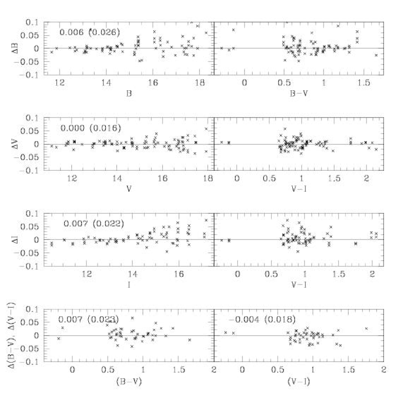
Figure 1: Photometric residuals [in the sense of our values minus those of Landolt (1992) and Stetson (2000)] from the calibration of primary standard stars. The RMS residuals are listed in the panels (with the standard deviations given in parentheses). The number of stars in the respective plots are 75 in $\Delta B$, 89 in $\Delta V$, and 68 in $\Delta I$.

where $b$, $v$, and $i$ are the observed aperture photometry magnitudes, $B$, $V$, and $I$ are the standard system magnitudes, and $X$ is airmass. The transformation coefficients were determined using the program CCDSTD (e.g. Stetson 1992). While it was clear that higher order color terms would be necessary to adequately fit measurements of extremely red stars ($\bv>2.0$), we found that such terms were unnecessary because the cluster stars fell in a range of colors that was quite well fitted by linear color terms. Our calibrated measurements for the standard stars are compared to the catalog values are shown in Figure 1.

2.4 Calibration Against Secondary Standards

Observations in each filter of the cluster fields were made on night 6, and used to calibrate the cluster data. We selected 193 stars with relatively low measurement errors from the outskirts of the cluster as our local standards. These stars were generally on the asymptotic giant branch, upper RGB, or horizontal branch (HB), and covered the entire range of colors for the cluster stars observed. We used the photometric transformations above to derive standard values for these stars.

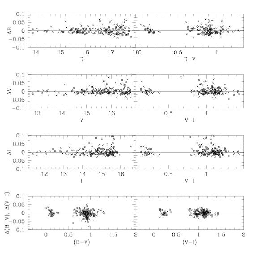
Figure 2: Photometric residuals (in the sense of the final point-spread function photometry minus standard aperture photometry values) from the calibration of secondary standard stars.

The calibrated secondary standard values were then used to calibrate the PSF-fitting photometry. PSF-fitting photometry from both nights of M12 observations were combined and averaged after zero-point differences between frames had been determined and taken into account. We then verified that the linear color terms derived earlier accurately corrected our data for color-dependent systematic errors (see Figure 2), and determined zero-point corrections for the photometry in each filter band. As a final note, we did not include the measurements of the brightest calibrated stars from the longest exposed $V$-band frames in order to avoid introducing systematic errors from non-linearity near CCD saturation.

2.5 Comparison to Previous Studies

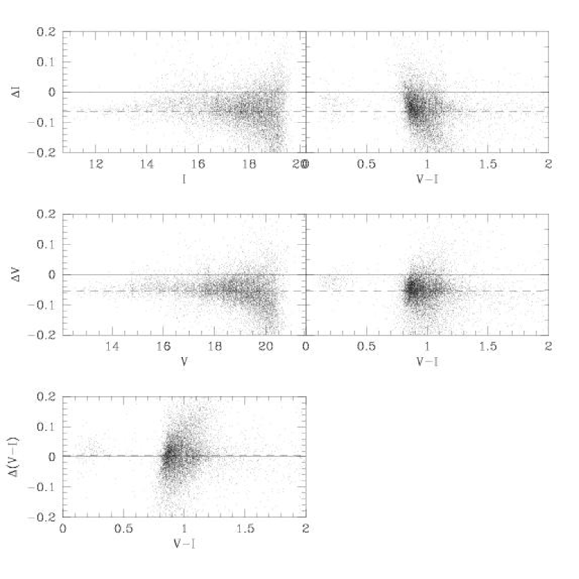
Figure 3: Residuals (in the sense ours minus theirs) from the star-by-star comparison of our photometry with that of von Braun et al. (2002). The dashed line represents the median value of all points.

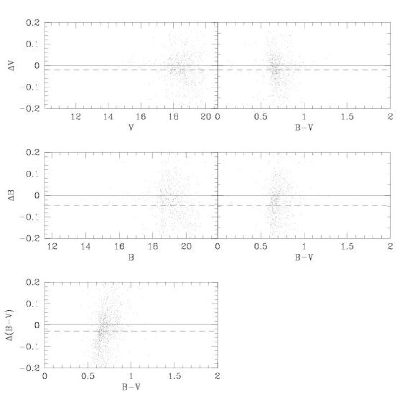
Figure 5: Residuals (in the sense ours minus theirs) from the star-by-star comparison of our photometry with that of Brocato et al. (1996). The dashed line represents the median value of all points.

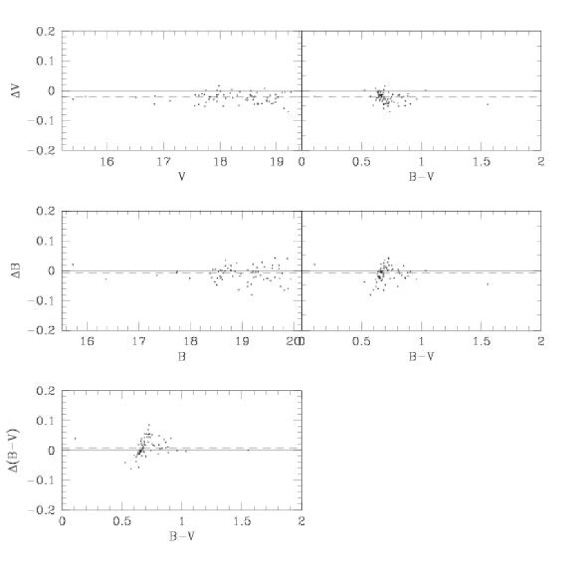
Figure 6: Residuals (in the sense ours minus theirs) from the star-by-star comparison of our photometry with the local standard stars of Stetson (2000) in this cluster. The dashed line represents the median value of all points.

In order to check the accuracy of our photometric calibration, our data set was compared (star-by-star) to recent ground-based data from R00, VB02, and B96. Figures 3 and 4 show the $V,I$, and $(V-I)$ photometric residuals (our data minus theirs) from comparisons with the VB02 and R00 studies, respectively. Figure 5 shows the $V$ and $(B-V)$ residuals from comparison with the B96 data. In Table 1 we provide the median values of these residuals, since this statistic is less sensitive to “outliers” than the mean. Our data agree (within reasonable errors) with both the B96 and R00 data. The VB02 photometry is significantly faint compared to ours. Because the median of the residuals ranges from $0.02$ to $0.06$ magnitudes, we also compare our data to the Stetson (2000; denoted S00 in Table 1) local standard stars in this cluster and show the residuals in Figure 6. This comparison yields small median residuals showing consitent photometric calibration between this study, the Stetson (2000) local standards, and the B96 & R00 data sets.

3 The Color Magnitude Diagram

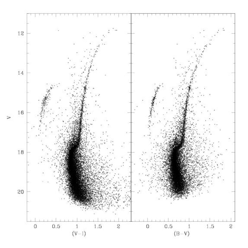
Figure 7: $V,(V-I)$ and $V,(B-V)$ CMDs for all 17,303 stars measured in this study.

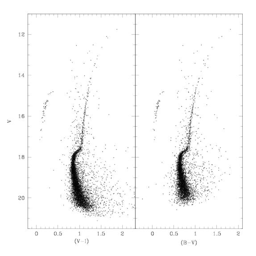
Figure 8: $V,(V-I)$ and $V,(B-V)$ CMDs for the sample of measured stars restricted to having a radius between 3^′.4 and 8^′.5 from the cluster center.

The results of this $BVI$ photometric study are presented as CMDs in Figures 7 and 8. The total sample of 17,303 stars measured in this study is shown in Figure 7. Given the lack of structure in the CMD beyond 8^′.5, in our final sample we ignored stars beyond this radius from the cluster center. Figure 8 shows the CMDs of the cluster restricted to those stars located between a radius of 3^′.4 and 8^′.5 from the cluster center. We derive fiducial sequences for both the $V,(B-V)$ and $V,(V-I)$ CMDs, and present the data in Tables 2 and 3, including the number of stars $N$ in each bin used to compute the fiducial point. For the MS, the fiducial sequence was determined by taking the mode of the color distribution in magnitude bins. The SGB fiducial points were also determined by finding the mode of the magnitude distribution in color bins because of the horizontal nature of the SGB in the CMD. The mean of the color distribution was used to compute fiducial points for the RGB. The mean of the distribution in a combination of color and magnitude bins were used to compute the fiducial points for the HB.

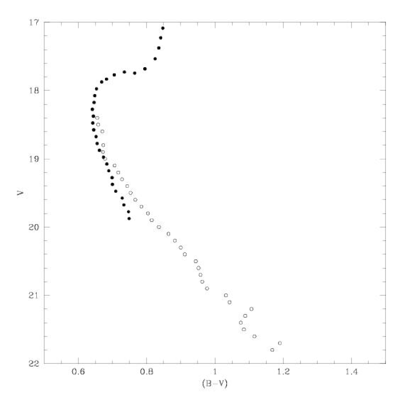
Figure 9: Comparison of the fiducial sequence derived in this study (filled circles) with that of Sato, Richer, & Fahlman (1989) (open circles).

In Figure  9, we compare our derived $V,(B-V)$ fiducial sequence with that of S89. Their $UBV$ photometric study of M12 presents the only recent fiducial sequence available for comparison to our data set. We attribute the differences in the slope and offset of the MS fiducials to differences in the photometric calibrations, although this is difficult to verify since no other published study has done star-to-star comparisons with the S89 dataset.

4 Cluster Parameters: Metallicity, Reddening, Distance Modulus, and Age

In this section we describe our method for the determination of four cluster parameters (metallicity, reddening, distance modulus, age) necessary to compare the theoretical LF to the observed.

4.1 Metallicity

There have been a number of [Fe/H] studies of M12, and published values range over nearly $0.5$ dex. The two most widely used metallicity scales are those of Zinn & West (Zinn & West 1984; Zinn 1985; hereafter ZW) and Carretta & Gratton (1997; hereafter CG). ZW cite a value of [Fe/H]$=-1.61$. The CG scale (based on high-resolution spectroscopy of GGC red giants) gives [Fe/H]$=-1.37$ from the quadratic transformation of the ZW scale. The discrepancy between the two scales is well-documented, with the CG scale giving a higher metallicity by approximately $0.2-0.3$ dex for low- or intermediate-metallicity clusters (such as M12) and approximately $0.1$ dex lower abundances for metal-rich clusters. Spectroscopic measurements of the infrared Ca II triplet of M12 red giants have been made by Suntzeff et al. (1993) and Rutledge et al. (1997). Rutledge, Hesser, & Stetson (1997) used these measurements to compute abundances on the ZW and CG scales of [Fe/H]${}_{ZW}=-1.40\pm 0.07$ and [Fe/H]${}_{CG}=-1.14\pm 0.05$. Recent work by Kraft & Ivans (2003) finds a metallicity of $\textrm{[Fe/H]}_{KI}=-1.25$ from observations of the equivalent width of Fe II in cluster red giants and calibration with $W^{\prime}$ from Rutledge, Hesser, & Stetson (1997). For the remainder of this study, we only consider metal abundances of M12 between $-1.40<\textrm{[Fe/H]}<-1.14$.

4.2 Reddening

In this study we adopt the reddening values as determined by VB02. They note the lack of significant differential reddening across the field of M12, and hence we do not use their maps to internally deredden our data. We use their mean reddening value of $E(V-I)=0.25$ that is in agreement with the infrared dust emissivity maps of Schlegel, Finkbeiner, & Davis (1998) who also find $E(V-I)=0.25$. Other measured values for the cluster reddening range from $E(B-V)=0.17-0.23$ (Racine 1971; S89). Given the agreement between the VB02 and Schlegel et al. (1998) studies, we adopt a value of $0.02$ as the uncertainty in the reddening.

4.3 Distance Modulus

Previous determinations of the distance modulus $(m-M)_{V}$ of M12 have yielded a wide range of values, from $(m-M)_{V}=14.02$ (VB02) to 14.30 (Racine, 1971). Even between studies that adopt similar techniques to find the distance modulus (namely subdwarf fitting) the results are not in agreement: the study by S89 finds $(m-M)_{V}=14.25\pm 0.20$ but Saad & Lee (2001) find $(m-M)_{V}=14.03\pm 0.11$. Given that the overall uncertainty in previous distance determinations is inadequate to define a well-constrained range, we use the technique of subdwarf fitting to re-determine the distance modulus of M12. Because the data in this study are mostly drawn from the evolved stellar populations, our MS is not faint enough to be adequate for this fitting technique. To overcome this, we use the VB02 data which goes several magnitudes fainter and has a well-defined MS. Fiducial points (listed in Table 4) for the main sequence were determined using methods identical to those described in $\S 3$, after correcting the data for the median offsets in Table 1. In order to minimize the possibility of systematic effects in the distance determination, we adopt the CG metallicity scale for both the subdwarfs and M12. We limit our sample of possible subdwarfs to those that have well-determined parallaxes $\pi$ (specifically those with relative error $\sigma_{\pi}/\pi<0.12$). This list was further restricted to stars that have metallicities measured on the CG scale. This subset was further limited by lack of $I$-band photometry: measured $V-I$ colors are sparse for metal-poor subdwarfs in the literature. From these considerations, our list of subdwarfs has magnitudes in the range $4.56<M_{V}<7.17$, metallicities between $-1.79<$[Fe/H]$<-0.90$, and relative parallax errors $\sigma_{\pi}/\pi<0.08$.

These 13 potentially usable subdwarfs are listed in Table 5. Columns 1 and 2 list the Hipparcos Input Catalog number and HD (or Gliese) number, respectively. Columns 3 and 4 list the reddening $E(B-V)$ and apparent $V$ magnitude, as compiled by Carretta et al. (2000) from the photometry of Carney et al. (1994); Ryan & Norris (1991); Schuster & Nissen (1989) and the Hipparcos catalog. Columns 5 and 6 give the Hipparcos parallax $\pi$ (in units of milliarcseconds) and the relative parallax error $\sigma_{\pi}/\pi$, both taken from the catalog. The absolute $V$ magnitude $M_{V}$ is listed in column 7 (and its error $\sigma_{M_{V}}$ in column 8) and includes the Lutz-Kelker corrections following the procedure described by Hanson (1979). The observed $(V-I)$ colors in column 9 are taken from Dean (1981), Mandushev et al. (1996), and Reid et al. (2001). The metal abundance [Fe/H] on the CG scale from Carretta et al. (2000) is listed in column 10. The deviation between the observed subdwarf color and the theoretically predicted color, denoted as $\delta(V-I)$, is listed in column 11. Column 12 shows the subdwarf colors after application of the theoretical color correction. For our MS fit, we use only those subdwarfs having metal abundances in the range $-1.50<\textrm{[Fe/H]}<-1.20$, following the discussion in VandenBerg et al. (2000, 2002). They note the excellent agreement of the observed and theoretical colors for the subdwarfs in this range. Our results confirm this agreement; the mean deviation of the observed and theoretical colors is $0.004$ for the six subdwarfs in this range. Our final list of 6 subdwarfs used in the fit have absolute magnitudes $M_{V}>5$, metallicities between $-1.48<$[Fe/H]$<-1.24$ (mean of $-1.35$), and relative parallax errors $\sigma_{\pi}/\pi<0.070$. We emphasize that this analysis assumes an $\alpha$-element abundance enhancement of $[\alpha$/Fe]$=+0.3$ for each subdwarf and negligible age differences.

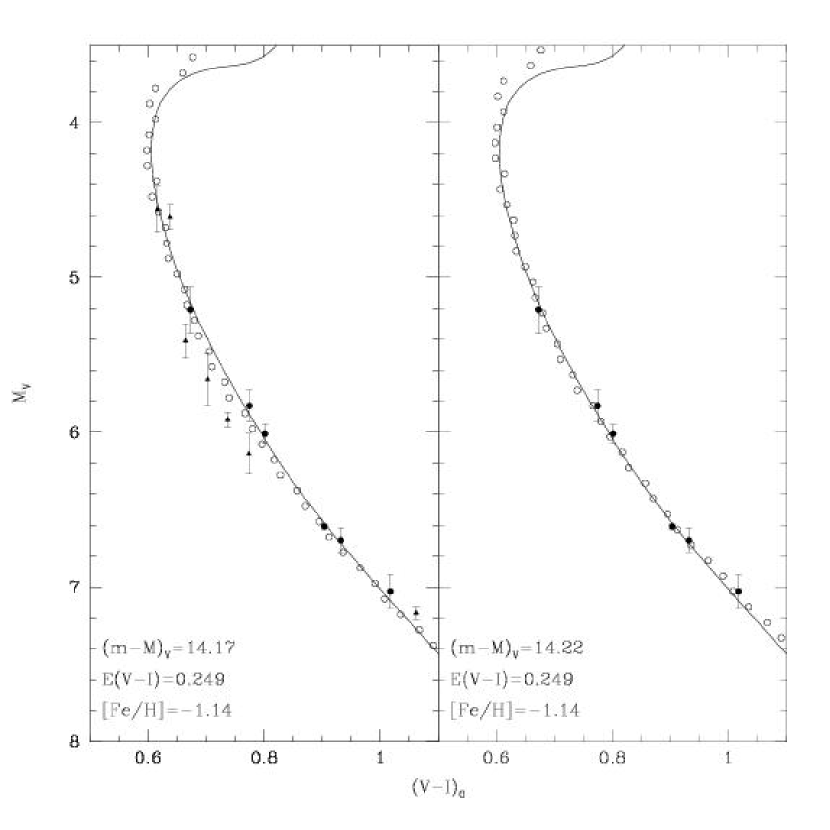
Figure 10: Example of the subdwarf fitting performed on the MS fiducial of von Braun et al. (2002) (open circles). The fiducial points have been shifted to the derived value of $(m-M)_{V}$. Overlaid on the subdwarfs (filled circles) is the 12 Gyr isochrone from Bergbusch & VandenBerg (2001) (solid line) for a metallicity of [Fe/H]$=-1.14$. The left panel shows the fit using all 13 subdwarfs; the right panel shows the fit using the restricted set of 6 subdwarfs. Those subdwarfs denoted as triangles were eliminated from the final distance modulus determinations.

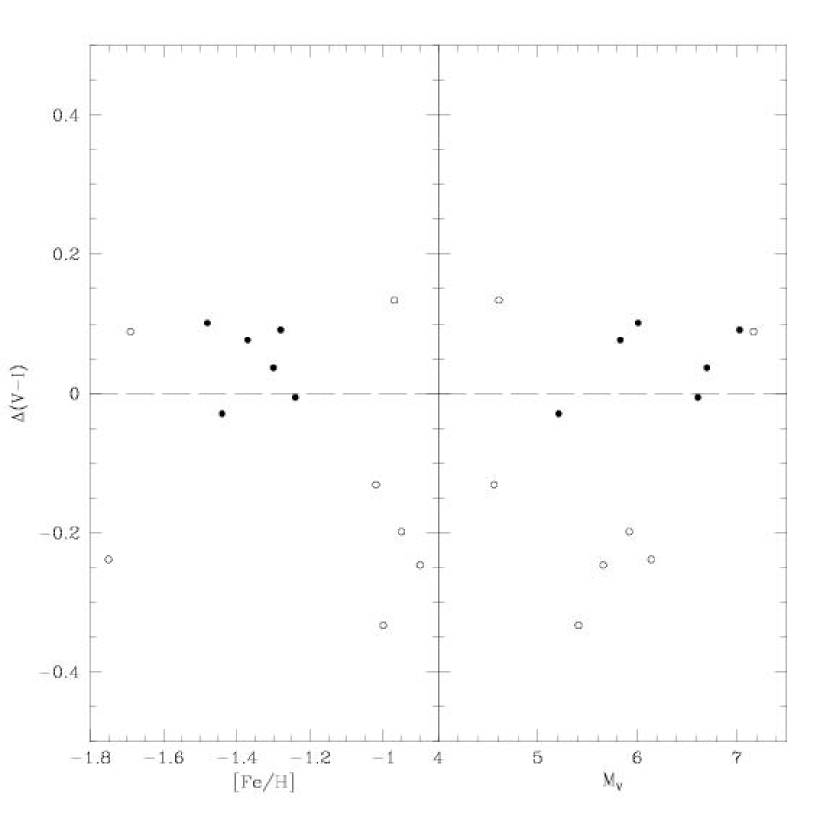
Figure 11: Residuals to the distance modulus fit in Figure 10 as a function of metallicity and absolute $V$ magnitude. The stars denoted as open circles (which correspond to the triangles in Figure 10) were eliminated from the final distance modulus determinations.

Figure 10 shows the best fit of the M12 fiducial to these stars, along with a 12 Gyr isochrone from Bergbusch & VandenBerg (2001; hereafter BV) for $\textrm{[Fe/H]}=-1.14$. The derived distance modulus changes depending on which set of subdwarfs are selected [$(m-M)_{V}=14.17$ for all 13 subdwarfs; $(m-M)_{V}=14.22$ for our final list of 6 subdwarfs]. We used a polynomial interpolation between several 12 Gyr isochrones of BV to determine a theoretical color correction for each subdwarf. This correction is computed as the difference at the $M_{V}$ of the subdwarf between the colors of isochrones having the metallicity of M12 and the metallicity of the subdwarf. In order to fit for the distance modulus, the fiducial of M12 is shifted in magnitude to match each subdwarf individually. Thus, each subdwarf provides a measure of the distance modulus and our final estimate is a mean value weighted by the squares of the error estimates of the absolute magnitude. These error estimates include the uncertainties in the subdwarf’s parallax, reddening, and metallicity. We assume an uncertainty in the metallicity of each subdwarf of 0.1 dex. The derived apparent distance modulus of M12 (assuming a metallicity of [Fe/H]$=-1.14$) is $(m-M)_{V}=14.22\pm 0.11$ using the six subdwarfs in Table 5. We plot in Figure 11 the difference between the theoretically corrected subdwarf color and the M12 fiducial color (at the absolute $V$ magnitude of the subdwarf), denoted as $\Delta(V-I)$, as a function of metallicity and absolute $V$ magnitude. These show no significant systematic errors from the fit. The largest uncertainty in the distance modulus comes from the adopted cluster metallicity. For metallicities [Fe/H]$=-1.41$ and $-1.61$, we find distance moduli of $(m-M)_{V}=14.05\pm 0.12$ and $13.96\pm 0.11$, respectively.

In order to check for possible systematic errors in the subdwarf color corrections, we perform the same procedure of subdwarf fitting using the Yonsei-Yale isochrones from Kim et al. (2002; hereafter Y²) to obtain the theoretical color correction to the subdwarfs. We use the color transformation table of Green, Demarque, & King (1987) (hereafter G87) to avoid introducing any systematic errors from use of the Lejeune, Cuisinier, & Buser (1998) (hereafter L98) table, which clearly differs from both the BV color transformation and the G87 table at faint absolute magnitudes. Using the Y² isochrones with the G87 tables, we find an apparent distance moduli of $(m-M)_{V}=14.23\pm 0.11,14.05\pm 0.12$ and $13.94\pm 0.12$ for metallicities of [Fe/H]$-1.14,-1.41,$ and $-1.61$. These are in excellent agreement (within the errors) to the value derived from the BV isochrones.

4.4 Age

The latest studies of the cosmic background radiation data from WMAP have found the age of the universe to be $13.7\pm 0.2$ Gyr (Spergel et al., 2003), setting a tight upper-limit on the possible ages of GGCs. Using the relative age indicator $\Delta V_{\textrm{{to}}}^{\textrm{{hb}}}$ (defined as the difference between the $V$ magnitude of the ZAHB and MSTO points), the Rosenberg et al. (1999) study (which uses the R00 homogeneous data set) deduces a value of $\Delta V_{\textrm{{to}}}^{\textrm{{hb}}}=3.60\pm 0.12$ for M12. They find M12 to be coeval (within the errors) with the oldest clusters that have metal abundances [Fe/H]$<-1.2$. Salaris & Weiss (2002) use both relative and absolute age dating (with the R00 data set) and find ages of $12.5\pm 1.3$ Gyr or $12.7\pm 1.3$ Gyr for metallicities of $\textrm{[Fe/H]}_{CG}=-1.14$ or $\textrm{[Fe/H]}_{ZW}=-1.40$, respectively, for M12. Both Rosenberg et al. (1999) and Salaris & Weiss (2002) find an age dispersion for clusters of intermediate metallicities (possibly as high as 25%) but the study by VandenBerg (2000) finds this dispersion to be smaller. Assuming the age of M12 to be coeval (or nearly coeval) with these oldest clusters and allowing for a possible age dispersion, we consider the range of possible ages of M12 to be between 11 and 13 Gyr. We discuss age further in §6.

5 Determination of the Luminosity Function

5.1 Artificial Star Tests

In order to properly determine an accurate LF a calculation of incompleteness corrections must be made. To quantify the incompleteness as a function of both magnitude (corrections for faintness) and radius (corrections for crowding), extensive artificial star tests have been performed. We mostly follow the prescription given by Sandquist et al. (1996) for the calculation of incompleteness corrections and here simply present a review of the methodology as it applies to our data set.

The artificial star tests were restricted to the $V$ and $I$ frames. A theoretical LF was used to set the distribution of artificial stars as a function of magnitude. The fiducial line gives the corresponding $I$ magnitude for an input $V$ magnitude from the theoretical LF. Artificial star magnitudes were chosen to create a sufficient number of bright stars, while weighting the distribution to the faint end of the CMD. Positions for the artificial stars are chosen at random within a grid such that no artificial stars can overlap (separations are no closer than $2\times($PSF radius$)+1$ pixels). The central portion of the grid is twice as dense as the outer portion, and hence will place a higher percentage of artificial stars in the most crowded regions of the cluster. The grid itself was randomly shifted by a fraction of a bin width from run to run. The ADDSTAR routine from DAOPHOT was used to add properly-scaled PSFs to the frames. Approximately 2,100 stars were added per frame in an individual artificial star run. The frames with artificial stars are reduced in a manner identical to our initial photometric procedures, and were compared to a control run that had no artificial stars. We conducted 39 artificial star runs that resulted in total of 84,400 stars being placed and reduced.

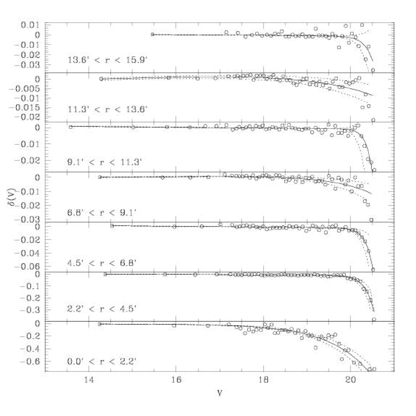
Figure 12: Results from the artificial star tests for the magnitude bias in the $V$ band $\delta(V)$ as a function of radius and magnitude.

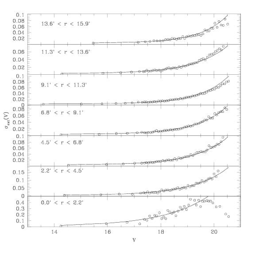
Figure 13: Results from the artificial star tests for the external $V$ magnitude errors $\sigma_{ext}(V)$ as a function of radius and magnitude.

The output from the artificial star runs is a list of positions and magnitudes for all detected stars. What qualifies as a detection is non-trivial; blending and crowding of artificial stars with real stars will tend to favor the detection of the brightest stars (in a simple positional search) regardless of whether or not they were artificial (see Sandquist et al. (1996) for more details). The resulting list of recovered artificial stars is used to calculate the following quantities (in bins sorted by projected radius and magnitude): (1) median $V$ or $I$ magnitude, (2) median color $(V-I)$, (3) median internal error estimates ($\sigma_{V},\sigma_{I},\sigma_{(V-I)}$), (4) median magnitude and color biases ($\delta_{V}\equiv\textrm{median}~{}(V_{\textrm{\small{output}}}-V_{\textrm{\small{input}}}),\delta_{I},\delta_{(V-I)}$), (5) median external error estimates ($\sigma_{\textrm{\small{ext}}}(V)\equiv\textrm{median}~{}|\delta_{V}-\textrm{median}~{}(\delta_{V})|/0.6745,\sigma_{\textrm{\small{ext}}}(I),\sigma_{\textrm{\small{ext}}}(V-I)$), and (6) total recovery probabilities ($F(V),F(I)$; the fraction of stars added that were recovered at any magnitude). In order to obtain an estimate of these quantities beyond the magnitude limit of the tests, we fit these quantities with the functional forms given in Sandquist et al. (1996) and computed errors following the procedure in Sandquist et al. (1999). Figures 12-13 present the results of the above calculations for 200 pixel ($2\farcm 3$) radial bins in both $V$ and $I$ bandpasses.

5.2 The Observed Luminosity Function

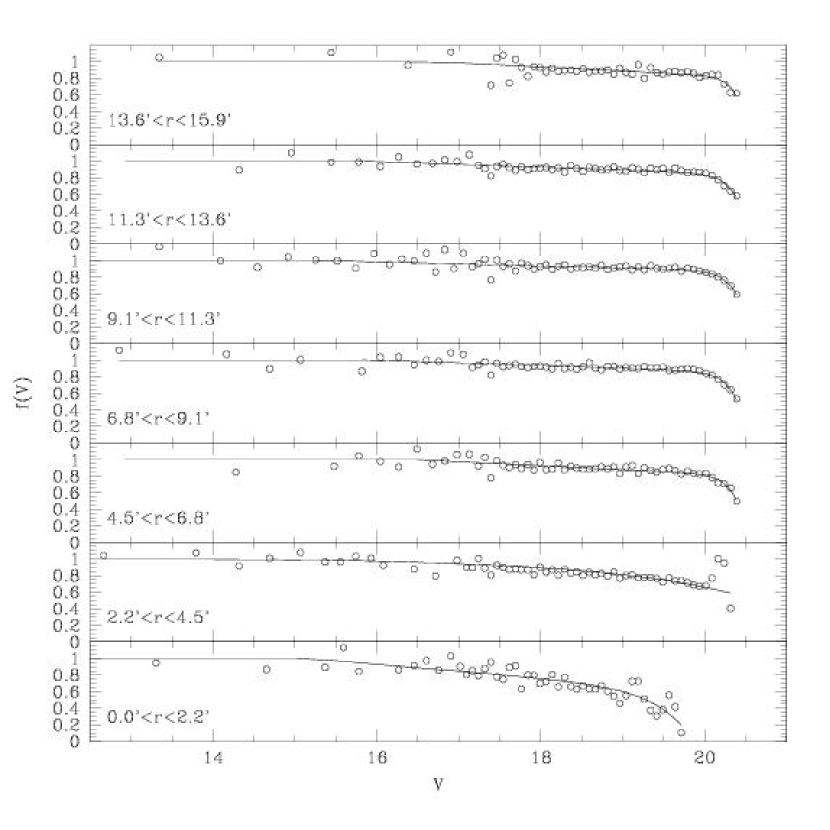
Figure 14: Results from the artificial star tests for the completeness fraction in the $V$ band as a function of magnitude and radius.

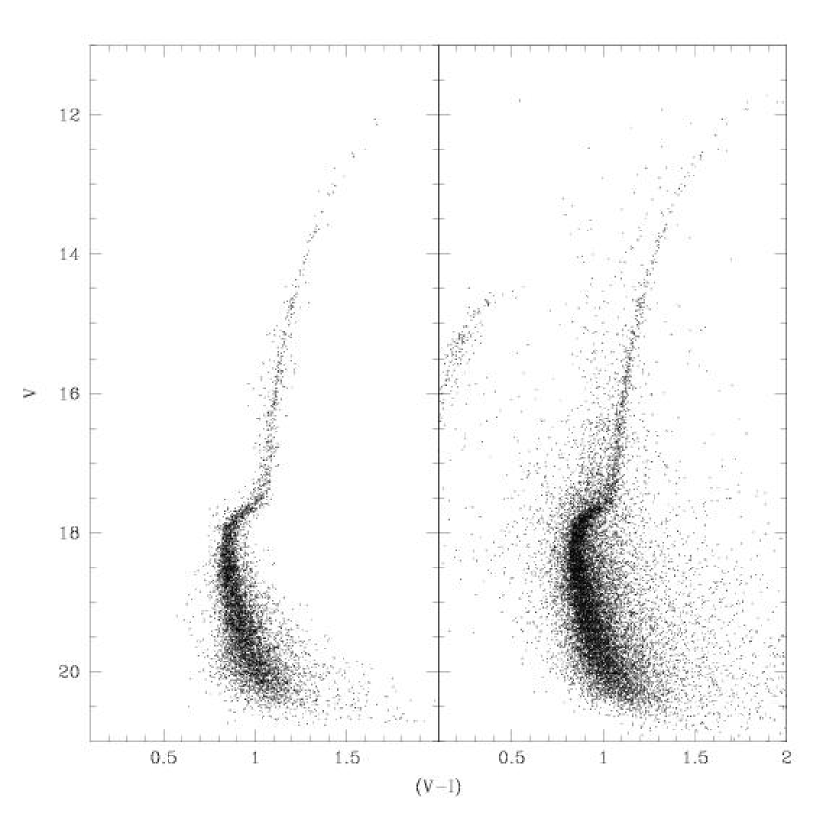
Figure 15: Comparison of the stars kept (left panel) out of the total sample of star (right panel) for the artificial star tests.

From the results of the artificial star tests we determined the corrections to the observed LF, following the procedure of Sandquist et al. (1996) that is based on work of Bergbusch (1993), Stetson & Harris (1988), and Lucy (1974). In the computation of the LF the error distributions, magnitude bias, and recovery probability are used to predict the form of the observed LF when given an initial estimate of the “true” LF. Once the true LF is determined, the completeness correction $f$ can be calculated as simply the ratio of the predicted number of observed stars to the actual number of observed stars. The values of $f$ for the various radial bins were fit using the same functional form as $F$, and are plotted in Figure 14. The total LF was calculated using the completeness factor (multiplying each star by the value $f^{-1}$ corresponding to its projected radius) and binned. In Tables 6 and 7 we present the observed $VI$ band LF derived in this study, including the upper and lower $1\sigma$ error bars ($\sigma_{high}$ and $\sigma_{low}$, respectively). Figure 15 shows the CMD of those stars kept for the determination of the LF compared to the original sample.

6 Comparison to Theoretical Models

6.1 The Color Magnitude Diagram

Using the parameters derived in $\S 4$, we compare our data to the BV and Y² theoretical isochrones. For the Y² models (Version 2), we compared our data to the isochrones computed using both the G87 and L98 $T_{\mbox{eff}}$-color transformation tables. Also included in this comparison is the intermediate metallicity isochrone from VandenBerg et al. (2002) (from the models of Richard et al. (2002) and Turcotte et al. (1998); hereafter denoted as the Richard & VandenBerg model). The BV and Richard & VandenBerg isochrones are computed from identical $T_{\mbox{eff}}$-color transformation relations which are a preliminary version of those presented by VandenBerg & Clem (2003; D. A. VandenBerg 2004, private communication). All isochrones have been computed assuming an $\alpha$-element abundance enhancement of $[\alpha$/Fe]$=+0.3$. The differences between the input physics of the models are noted in Table 8.

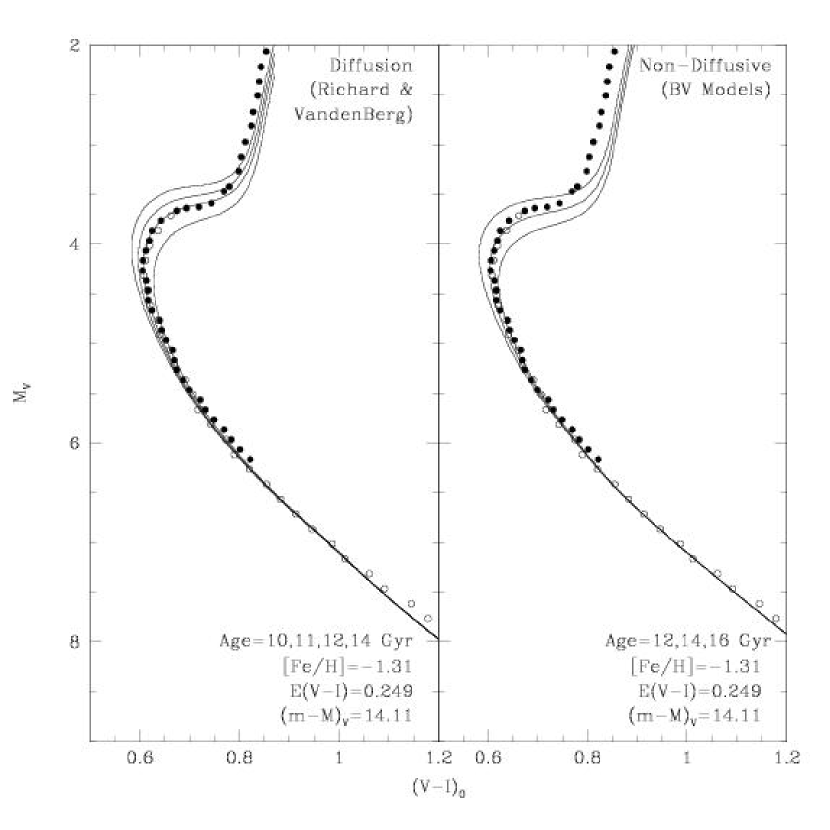
Figure 16: Comparison of the fiducial points derived in this study (filled circles are our data; open circles are the von Braun et al. (2002) data) with theoretical isochrones. No offset has been applied to the observed colors.

In Figures 16 and 17 we plot our fiducial sequences (using the determined distance modulus and reddening) against the three models described above. Following VandenBerg (2000), the isochrones have been shifted by an amount $\delta$ in order to align the colors at the main sequence turnoff (MSTO). This small shift ($\delta\sim 0.02$ for the Y² models and $\delta=0.001$ for the BV models) accounts for small differences in color that may arise from photometric zero-point differences, $T_{\mbox{eff}}$-color discrepancies, or reddening errors. Given these shifts, we note the inability of the Richard & VandenBerg, BV, and Y² L98 models to correctly predict the colors of the RGB fiducial sequence. For the cluster metal abundance we adopt [Fe/H]$=-1.31$ (close to the CG value) in order to make a direct comparison to the Richard & VandenBerg model. Previous work (Bergbusch & VandenBerg, 2001; VandenBerg et al., 2002) has argued for the use of the ZW metallicity scale when comparing the BV models to observational data. If we assume [Fe/H]$=-1.61$ for the comparison to the BV models, we find that one would need an 18 Gyr isochrone in order to match the fiducial sequence. Similarly, if we assume this metallicity for the comparison to the Y² models, we find that one would need a 16 Gyr L98 Y² model isochrone or a 16-17 Gyr G87 Y² model isochrone to match the fiducial sequence. These ages are clearly above the recent WMAP upper-limit; in order to obtain a reasonable age of 13 Gyr given the metallicity on the ZW scale, the distance moduli would need to be larger by $2-3\sigma$. Regardless of the differences in input physics between the BV and Y² models (and assuming our values for the distance modulus determined in $\S 4.3$), adoption of the ZW metallicity scale implies an age for M12 that is too old given recent constraints of the cosmic microwave background measurements (Spergel et al., 2003). As an estimate of the uncertainty in the deduced ages, we find that an error of approximately $\pm 0.1$ in $(m-M)_{V}$ (just below our $1\sigma$ error) can result in a change of $\pm 1.0$ Gyr in age. Comparisons of the observed $V,(B-V)$ fiducial points with these theoretical models implies identical ages for M12 to those deduced from Figures 16 and 17.

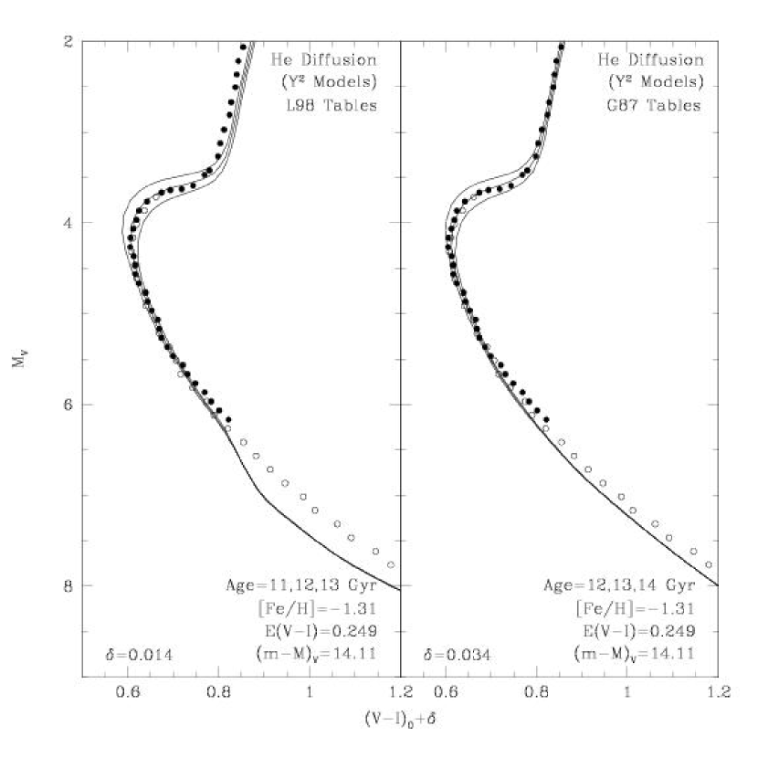
Figure 17: Comparison of the fiducial points derived in this study (filled circles are our data; open circles are the von Braun et al. (2002) data) with theoretical isochrones. Offsets of the amounts $\delta$ have been added to the observed colors to force agreement on the upper MS.

Given the adoption of the CG metallicity scale, Figures 16 and 17 show that the different models imply slightly different ages for the cluster. The Richard & VandenBerg and Y² models both imply reasonable ages ($12-13$ Gyr) for M12, while the BV models imply an older age by $\sim 1-2$ Gyr. This can most likely be attributed to the inclusion of gravitational settling in the Richard & VandenBerg and He diffusion in the Y² models and the lack of diffusive physics in the BV models. In comparing the Richard & VandenBerg and BV isochrones, the diffusive models mimic older non-diffusive isochrones (such as a shorter SGB) primarily because MS evolution is accelerated by the presence of additional He in and around the stellar core. This is in agreement with previous theoretical work done on the effects of He diffusion and GCC ages, as noted in $\S 1$. Comparing the two Y² models (see Figure 17) it should be noted that because the two Y² isochrones are calculated from identical input physics, the differences between these two can be solely attributed to the differences in the G87 and L98 $T_{\mbox{eff}}$-color tables. From the differences between Figures 16 and 17 one can see (not surprisingly) that differences in input physics (Richard & VandenBerg vs. BV) and color transformations (Y² G87 vs. Y² L98) both have a significant effect on the comparison of theoretical isochrones with observed fiducial lines. These differences are of comparable magnitude. As an example of the resulting problems, the choice in using the L98 or G87 color tables with the Y² models changes the implied age of M12 (assuming the correct distance modulus). The left panel of Figure 17 would imply an age of $\sim 12$ Gyr using the L98 tables, while the right panel (of the same figure) would imply an age of $\sim 13$ Gyr from using the G87 tables.

6.2 The Luminosity Functions

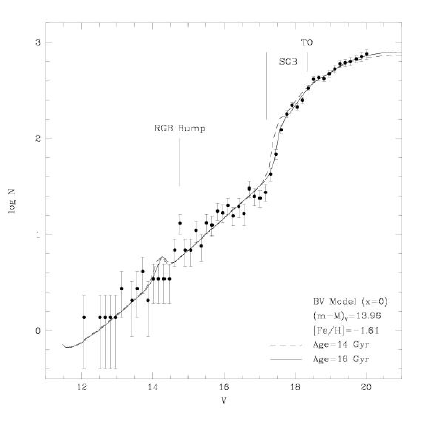
Figure 19: Comparison of the observed and theoretical (BV) $V$ band luminosity functions of M12. The ZW metallicity value has been chosen following the discussion in $\S 6.1$ and $\S 6.2$. A slightly older model (16 Gyr), or correspondingly larger distance modulus, provides a better description of the observed data.

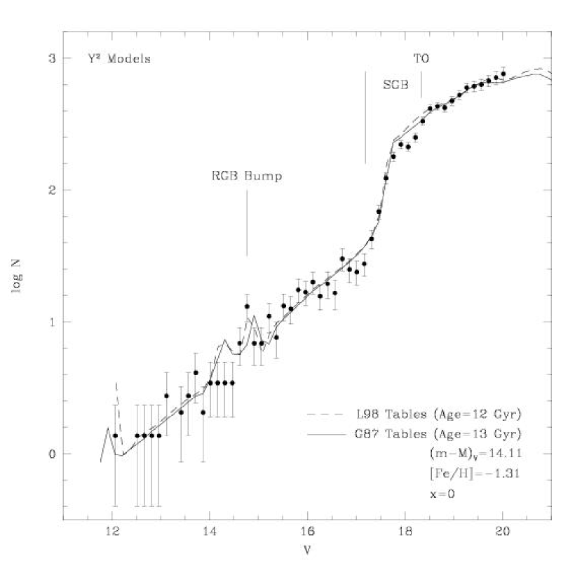
Figure 20: Comparison of the observed and theoretical (Y²) $V$ band luminosity functions of M12 for the two different ages implied by the G87 and L98 color transformation tables in Figure 17.

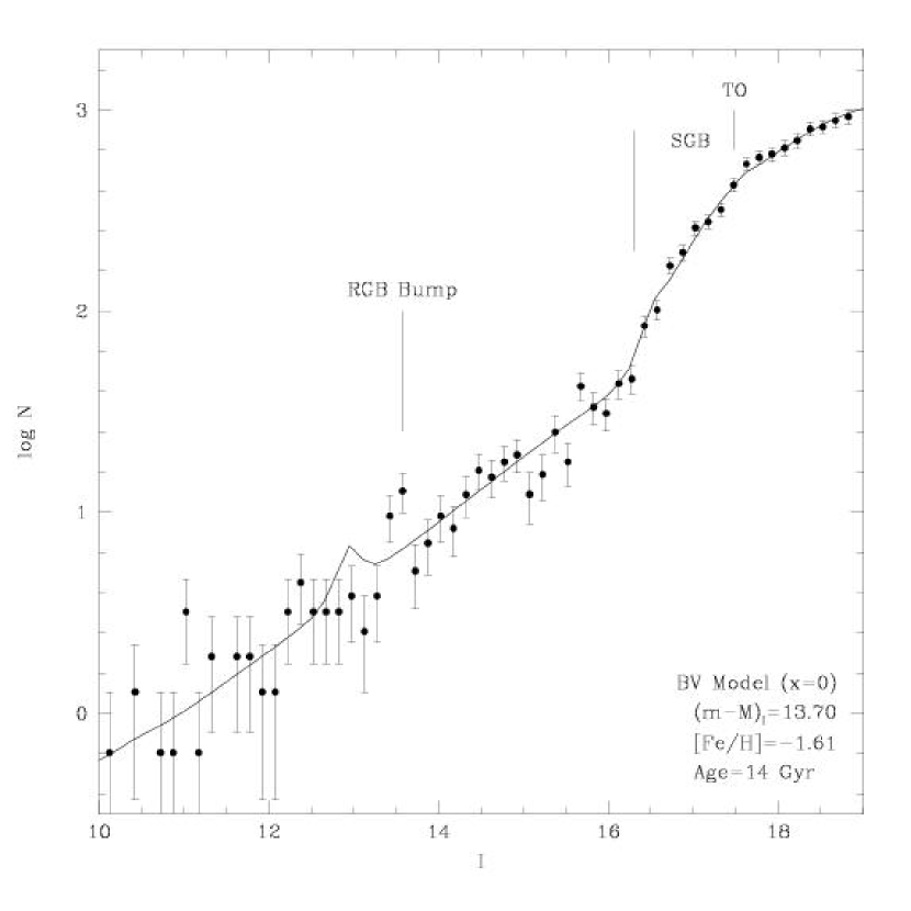
Figure 21: Comparison of the observed and theoretical (BV) $I$ band luminosity functions of M12.

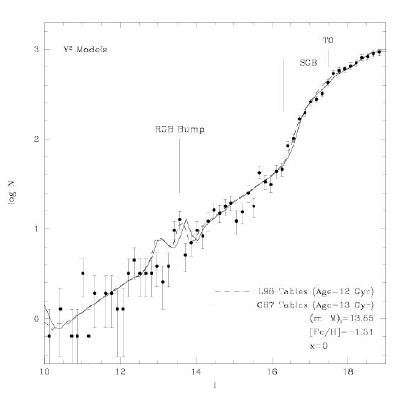
Figure 22: Comparison of the observed and theoretical (Y²) $I$ band luminosity functions of M12 for the two different ages implied by the G87 and L98 color transformation tables in Figure 17.

We compare the observed $V$ and $I$ LFs for M12 to theoretical LFs in Figures 18-22. In doing this, we wish to investigate whether the physics used in the theoretical models can adequately explain our observations. Theoretical LFs were generated for the BV and Y² models only, since LF data were not available from the Richard & VandenBerg models (D. A. VandenBerg 2003, private communication). Given the previous discussion over the metallicity scale and BV models (see $\S 6.1$) we show two comparisons of our observed $V$ band LF with the BV models, one for a cluster metallicity near the CG scale (Figure 18) and one for a metallicity on the ZW scale (Figure 19). For both these comparisons we show a 14 Gyr model as implied by the CMD in Figure 16. The LFs for this age should mimic younger diffusive models (see Proffitt & VandenBerg 1991 Figure 18). Despite the choice of metal abundance in the BV models we find that an age adjustment (or correspondingly a distance modulus change) is necessary in order to match the SGB “jump” in the $V$ band LF, although the adjustment is younger in one case (the CG metallicity; Figure 18) and older in the other (the ZW metallicity; Figure 19). The older age necessary for the ZW comparison is in agreement with the discussion in the previous section regarding the ZW metallicity scale; an older age (or larger distance modulus) to provide a better description of the data.

For LF comparisons with the Y² models (Figures 20 and 22), we adopt the metallicity of [Fe/H]$=-1.31$ because of the agreement of the Y² isochrones with the observed CMD for evolved stars (see Figure 17). In the $I$ band the shape of the Y² LFs is somewhat dependent on the choice of $T_{\mbox{eff}}$-color transformations, particularly in those regions where the CMD is changing the most (e.g. the MSTO and SGB regions). The $V$ band LF does not depend on the $T_{\mbox{eff}}$-color relations but only on the bolometric corrections. The various $V$ band distance moduli in Figures 18-22 were determined via subdwarf fitting (as in $\S 4.3$) assuming the value specific to the metallicity used for the theoretical model. The theoretical LFs were normalized (over a range of 0.3 mag) to the total number of stars in the M12 LF sample at a point on the upper MS $\sim 1$ magnitude fainter than the MSTO. A mass function exponent $x=0$ (where $N(M)\propto M^{-(1+x)}$) was selected as to match both the $V$ and $I$ band LFs at the faint end of the sample. This mass function exponent is in agreement with the one found by S89.

6.2.1 The Subgiant Branch

As noted in the introduction, some metal-poor clusters have shown evidence for an excess of stars on the SGB portion of the LF. In general the observed $I$ band SGB LF of M12 shows better agreement with theory than does the $V$ band SGB LF, which is noticeably “jagged” compared to the “smooth” theoretical models. Given that we have eliminated the faintest stars ($V<16$) in the core region of the cluster ($r<200$ pixels = 2^′.3), it is unlikely that stellar blends can account for the discrepant SGB LF. To test this possibility, we computed the $VI$ LFs for a restricted region of the data. After eliminating the core region ($r<250$ pixels = 2^′.8) we found no substantial difference in the observed LFs, thus justifying our radial cut in the LF computation. In our examination of the SGB region of the M12 LF we apply three different techniques in order to investigate the discrepancies between observations and theory:

• First we compare the theoretical and observed SGB LFs in an “absolute” fashion, using the values derived in $\S 4$ for the cluster parameters.

• Second, we make the SGB LF comparison after performing a shift to bring a common point on the upper MS into coincidence.

• Third, we formulate a technique to maximize the exploration of the evolutionary timescales of the cluster stars by selecting theoretical models based on compatibility with the observed CMD.

Lastly, we construct the LF of M12 from the HST data of Piotto et al. (2002) and compare this result with the LF derived in this study.

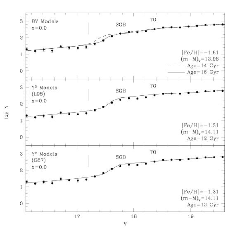
Figure 23: SGB region of Figures 19 and 20, showing the M12 $V$ band luminosity function with the BV and Y² theoretical models.

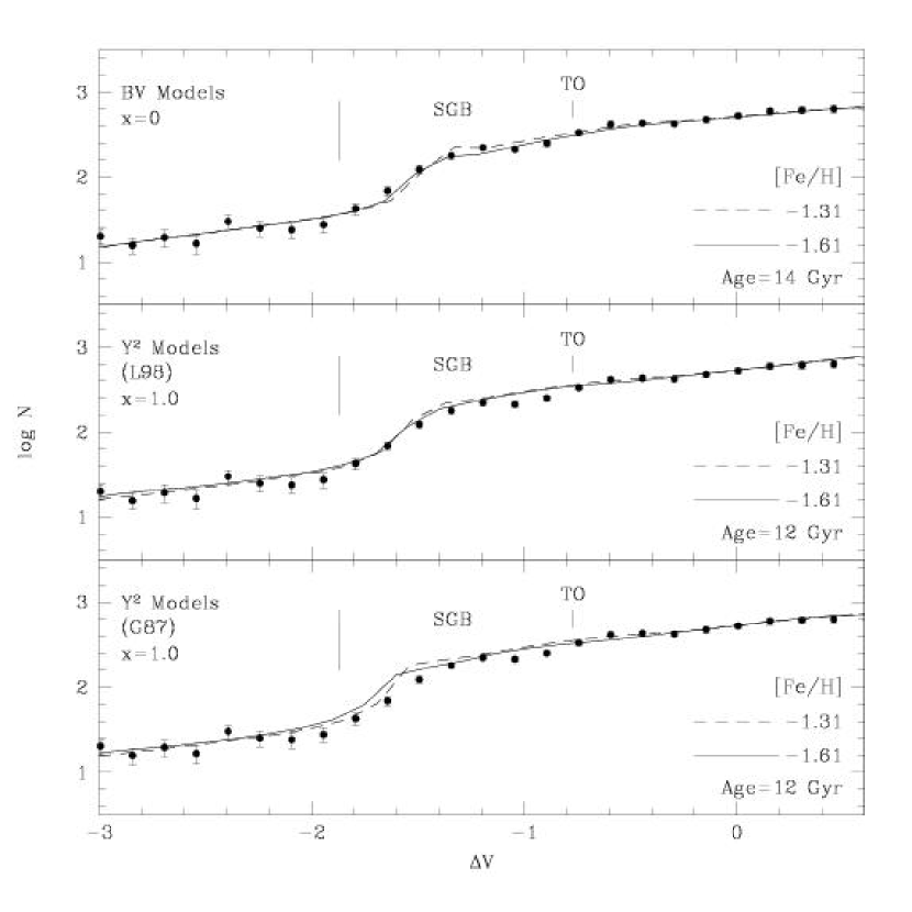
Figure 24: SGB region of the M12 $V$ band luminosity function shown with the BV and Y² theoretical models for two values of the cluster metallicity. The magnitude scale has been shifted to match a common point on the upper main-sequence as discussed in $\S 6.2.1$. The middle and bottom panels are identical except for the choice of color-$T_{\mbox{eff}}$ transformation table.

In Figure 23 we highlight the SGB and upper MS region of the M12 $V$ band LF with the same theoretical models from Figures 19 and 20. These comparisons use the parameters derived in $\S 4$, where the ages were adopted from the CMD analysis in $\S 6.1$. While the BV models appear to give the best overall description of the observed SGB region, this is only true if an older age (or larger distance modulus) is adopted (as noted in $\S 6.1$ and $\S 6.2$). In these “absolute” comparisons, both the Y² models predict more stars than are observed in the SGB LF bins between the SGB “jump” and the MSTO. Figure 24 shows the observed SGB region of the M12 $V$ band LF again, but here we use the second technique (listed above) for the comparison to theory. Figure 24 also shows theoretical LFs for metallicities on both the CG and ZW scale. In the theoretical models the SGB LF shapes are largely due to the choice of metallicity and age; the strongest dependence is usually on metallicity (Zoccali & Piotto, 2000). However, the choice of $T_{\mbox{eff}}$-color transformations also has a noticeable impact on the shape of the theoretical SGB LF. The Y² model comparisons in Figure 24 are identical except for the choice of color transformation table. Because of the strong correlation between metallicity, distance modulus, and age we shift the magnitude scale (of both the theoretical and observed CMDs) to bring a point on the upper MS into coincidence. We follow the method described by Stetson (1991), using as reference the point on the upper MS that is 0.05 magnitudes redder than the MSTO magnitude. In this formalism, the distance modulus has been eliminated and hence the age and metallicity will be difficult to determine (in an absolute sense) in such diagrams (Stetson, 1991). Uncertainties in the zero-pointing could be as high as $\sim 0.1$ mag, mostly because the slope of the upper MS differs between sets of isochrones. From Figure 24 we see that no choice of metallicity, color table, and model is able to completely describe the observed SGB LF. The BV and Y² models are able to match some points for a higher metallicity leaving other points lower than predicted, but a lower metallicity will mean other points are higher than predicted. Using the Y² models, a better description of the SGB region (that closely resembles the BV comparisons) can be found if a slightly larger mass function exponent $x=1$ is adopted (compare the SGB regions in Figures 23 and 24).

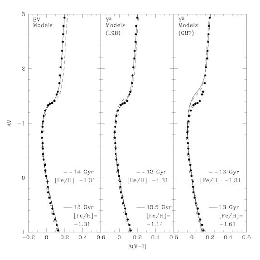
Figure 25: Comparison of the observed fiducial sequence of M12 with the BV (left panel) and Y² (middle and right panels) theoretical isochrones. Both the magnitude and color scales have been shifted to match a common point on the upper main-sequence as discussed in $\S 6.2.1$. The “best fit” isochrones from Figures 16 and 17 are shown as the dashed line, but we find the solid line theoretical models to better match the observations when the CMD is shifted in this manner. We are unable to find a Y² theoretical model (using the G87 color table and within the deduced range of cluster metallicity) that adequately describes the observed CMD.

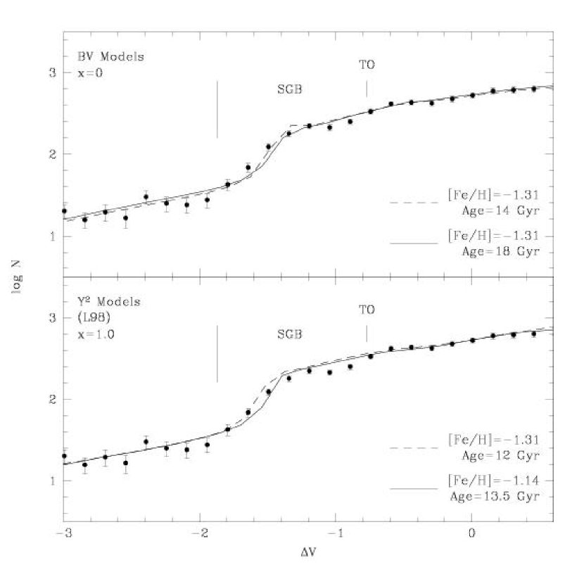
Figure 26: Comparison of the observed $V$ band LF of M12 and the BV and Y² (using the L98 color-$T_{\mbox{eff}}$ transformation table) theoretical LFs corresponding to the “best fit” isochrones in Figure 25 (solid line). The magnitude scale has been shifted to match a common point on the upper main-sequence as discussed in $\S 6.2.1$. The (dashed lines) theoretical models are identical to the dashed line theoretical models from Figure 24 and are plotted for comparison purposes.

Systematic errors in the $T_{\mbox{eff}}$-color transformations can lead to distortions of the theoretical isochrone in the observational CMD, and can thereby affect the theoretical LFs where the isochrone is changing most quickly in color. Independent of that, the slope of the subgiant branch in the theoretical HR diagram is affected by cluster parameters like age and metallicity. In order to minimize systematic differences between theoretical and observed LFs, and to attempt to focus on the evolutionary timescales of the stars, we devised another method of making the comparisons. In this method, we selected the theoretical isochrone that best matched the observed CMD fiducial sequence when shifting the magnitude and color scales to match a point on the upper MS (as described above). The theoretical model that best describes the observed CMD will be different depending on whether or not one performs this shift (or uses the determined distance modulus and reddening). While this technique places significant weight on the ability of the $T_{\mbox{eff}}$-color tables to correctly describe observations, it is unlikely that physical models will provide a good description of the observed LF if the theoretical and observed CMDs do not match. In Figure 25 we show the observed M12 fiducial sequence with the BV and Y² models when shifting the color and magnitude scale. The theoretical model that best described the observations using the “absolute parameters” in §6.1 (the dashed line in Figure 25) is shown with another model that better describes the fiducial sequence when performing this shift (the solid line in Figure 25). We are unable to find an adequate theoretical description of the CMD observations using the G87 color table with the Y² model (given the range of metallicity determined in §4.1). While this throws some doubt on the ability of the G87 tables to match observed colors, this should be further investigated for other GGC CMD observations. The metallicities required for the BV and Y² models are within the range of M12 observations previously quoted (§4.1), but the age of the BV model must be very large to match the shape of the SGB region of the fiducial line. Using the “best fit” BV and Y² L98 descriptions (from Figure 25), we show the observed M12 SGB LF with the theoretical LFs generated from these models in Figure 26. The theoretical LFs using our determination of the “absolute” parameters (i.e. the same theoretical LFs from Figure 24) are also shown. Neither set of models provides entirely adequate descriptions of the SGB region of the M12 LF. For the BV models, the SGB evolutionary timescale is somewhat underestimated. For the Y² models, the numbers of stars in the two magnitude bins just brighter than the MSTO point are more noticeably over predicted, and the slope of the LF for the bright SGB is predicted too steep.

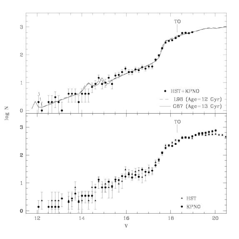
Figure 27: Top Panel: Luminosity function of M12 formed from combination of the HST data (Piotto et al., 2002) and the KPNO data (this study). Bottom Panel: The HST and KPNO data separately, with the HST data scaled to match the KPNO data at the upper main-sequence.

To further investigate the presence of over- or under-abundances of stars in the SGB region, we construct an M12 LF using a combination of our wide-field data with the HST photometry of Piotto et al. (2002). This summation of data sets will increase the statistical significance of the LF, while examination of the data set separated will allow for the inspection of the LF at differing radii from the cluster center. Figure 27 shows both the LFs separately and the combined LF compared with the Y² theoretical models of Figure 20. We only compute the combined LF down to $V=\sim 19$ in order to avoid complications with incompleteness in the HST data set. Two magnitude bins stand out when comparing the HST and KPNO data sets separately; the two bins just brighter than the MSTO appear to have more stars in the HST data than the KPNO data. If it is a “real” effect (e.g. not a computational artifact), then this would imply a larger number of SGB stars concentrated towards the cluster center. As can be seen in the combined (HST+KPNO) LF, the SGB region still shows a slight underabundance of stars compared to theoretical predictions. However, near $V=18.5$ (just fainter than the MSTO) there appears to be a small increase in the number of stars. In general, these discrepancies are small and at best statistically significant at $\sim 1\sigma$ level. As a judge of the goodness-of-fit, we compute the reduced $\chi^{2}$ (denoted $\chi_{\nu}^{2}$) for the two Y² models in Figure 27. For the 12 Gyr L98 Y² model we find $\chi_{\nu}^{2}=1.77$ and for the 13 Gyr G87 Y² model we find $\chi_{\nu}^{2}=1.55$. As a comparison between the KPNO and HST data, we find $\chi_{\nu}^{2}=2.85$. If we only compute $\chi_{\nu}^{2}$ for the MSTO and SGB regions of the LF ($17.3<V<19.0$ we find $\chi_{\nu}^{2}=4.57$ as a comparison between the KPNO and HST data, $\chi_{\nu}^{2}=2.99$ for the 13 Gyr G87 Y² model, and $\chi_{\nu}^{2}=4.07$ for the 12 Gyr L98 Y² model. In summary, the LF formed from the inclusion of the HST data set with our wide-field data still shows a discrepant SGB LF compared to theory.

6.2.2 The Red Giant Branch

The theoretical and observed $VI$ band RGB LFs appear to be in agreement within the errors for both the BV and Y². We note the detection of the RGB “bump” (in both the cumulative and differential LFs) at $V\sim 14.7$, $I\sim 13.6$. This is consistent with the $V$ magnitude of the bump determined by Ferraro et al. (1999). The observed $I$ band RGB LF agrees well for the most densely-populated portion fainter than the RGB bump ($13.4>I>16.2$, the “lower” RGB). Comparisons between the theoretical models show that the RGB slopes appear to be in good agreement. Noting the predicted and observed numbers of MS-to-RGB stars, there appears to be no discrepancy within the errors; M12 does not appear to have an excess of RGB stars compared to theory.

Both the BV and Y² models predict the presence of the RGB bump. The standard interpretation of the RGB bump is that it is due to the movement of the hydrogen burning shell through the chemical composition discontinuity left by the deepest penetration of the envelope convective zone (Thomas, 1967; Iben, 1968). The Y² models show two peaks near the observed RGB bump, but the brighter of the two peaks is the true RGB bump. The fainter, larger peak is a numerical artifact of the models due to luminosity grids which are sparse and non-uniform in this region of the models (S. Yi, private communication). Thus, both the BV and Y² predict a RGB bump at very similar magnitudes ($V=\sim 14.2$) but are $\sim 0.2$ magnitude brighter than actually observed. While this absolute comparison of the bump position disagrees with theory, recent work by Riello et al. (2003) has shown the bump position relative to the horizontal branch (for their sample of 54 GGCs) is in agreement with their most recent stellar evolution models.

6.3 Comparison of Theoretical and Observed LFs for Other Clusters

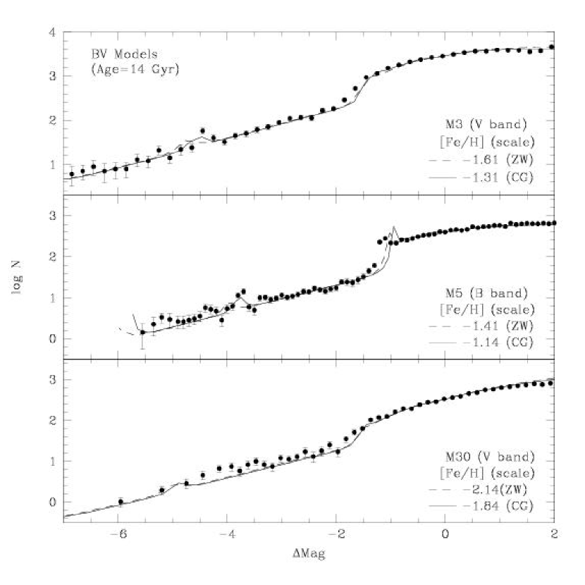
Figure 28: Comparison of the observed luminosity functions of M3 (top panel), M5 (middle panel), and M30 (bottom panel) with the BV theoretical luminosity functions. The magnitude scale has been shifted to match a common point on the upper main-sequence as discussed in $\S 6.2.1$.

Because of the influence of cluster metal abundance on the SGB morphology, we compare the BV and Y² theoretical models to the LFs of three other well-studied GGCs. In doing this we seek to make an attempt to determine whether one set of models can reproduce the main features of the LFs of clusters covering a wide range of metallicities. Figures 28 and 29 compare the observed LFs of M3 (Rood et al., 1999), M5 (Sandquist et al., 1996), and M30 (Sandquist et al., 1999) to theoretical LFs with metallicities from the ZW and CG scales. The mass function exponents were taken from the referenced studies: $x=0$ for M3, $x=0.5$ for M5, and $x=2.0$ for M30. The magnitude scale was shifted to a common zero-point as described above to eliminate the sensitivity to distance modulus and age. While this comparison does present clusters having a wide range of central densities, there is no evidence for population gradients in normal clusters and some evidence for this effect in post-core-collapse clusters (such as M30; see Burgarella & Buat (1996)). Given the radial cuts necessary to remove poorly-measured stars from the central regions of the clusters, the presence of crowding and possible population gradients should have a negligble influence on the shape of the cluster LFs.

The plots indicate that the SGB region is also somewhat insensitive to metallicity except for filter choices which the cause the SGB to be nearly horizontal, as is the case for the $B$-band LF of M5 (Sandquist et al. 1996). In the case of M5, the Y² theoretical LF using the ZW scale value is the most consistent with the observations. This feature might be exploited in future LF studies to help nail down the absolute metallicity scale. However, because the SGB is a feature primarily involving $T_{\mbox{eff}}$ change, current uncertainties in the $T_{\mbox{eff}}$-color transformations would have to be removed first. A comparison between the G87 and L98 tables for these clusters shows better agreement with observations when using the L98 transformations, as is also confirmed in comparing the middle and bottom panels of Figure 24. For all 3 clusters (and for M12 also), the BV models are unable to match the SGB jump and hence we are unable to choose between metallicity scales using these models.

Though the ZW scale is favored in these relative comparisons between theory and observations, in an absolute sense, the choice of the ZW metallicity scale in the M12 analysis means that the determined distance modulus will be too small to match our LF observations. (This is consistent with the discussion of the CMD $\S 6.1$.) The ZW scale implies that the use of an older model (or larger distance modulus) is necessary to match the cluster LF. We find that for a choice of [Fe/H]=-1.61, the Y² models must have age of 15 (using the L98 color table) or 16 (using the G87 color table) Gyr, respectively, to provide an adequate description of the M12 LF. To retain an adequate fit with a younger age of 13 Gyr and metallicity [Fe/H]=-1.61, the distance modulus would have to be larger that we determined by more than $2\sigma$. This should once again emphasize the importance of renewed attention to $T_{\mbox{eff}}$-color transformations.

7 Conclusions

In this paper we have presented the $VI$ luminosity functions (LFs) and $BVI$ color-magnitude diagrams (CMDs) of the Galactic globular cluster (GGC) M12 from wide-field CCD photometry. Given constraints on the cluster age, metallicity, distance modulus, and reddening we compare our data to three sets of theoretical stellar evolution models for metal-poor, $\alpha$-enhanced, low mass stars. We find that neither the Bergbusch & VandenBerg (2001) nor the Kim et al. (2002) models are able to adequately describe the SGB region of the M12 LF. While we find no statistically significant excesses of stars, the observed SGB LF has a noticeably different slope than predicted. We find the theoretical description of the SGB region of the cluster LF to be sensitive to the selection of color-$T_{\mbox{eff}}$ transformations, and to a lesser degree to age and metallicity. On the other hand, we find agreement between the observed and predicted numbers of MS-to-RGB stars; M12 does not appear to have an excess of RGB stars compared to theory. In the context of the Langer et al. (2000) claim that extremely blue (“second parameter”) clusters are explained by deep mixing (during the RGB phase) and resulting envelope helium enrichment, the M12 LF should have shown this RGB excess. In contrast to this, we find the LF to be similar to that of M3 [$(B-R)/(B+V+R)=0.08$; Lee et al.(1994)], another cluster of nearly identical metallicity that does not shown an excess of RGB stars. We find in our analysis that regardless of the differences in input physics in these two models, the adoption of the ZW metallicity scale is incompatible with observations. Assuming a metallicity for M12 on the ZW scale, adequate theoretical description of both the CMD and LF data would require either (1) a model older than recent estimates of the age of the universe (see below), or (2) a distance modulus that would be $2-3\sigma$ larger than we determined from subdwarf fitting.

Analysis of the WMAP experimental data (Bennett et al., 2003; Spergel et al., 2003) has now placed new restrictions to the age of the universe, and hence the possible ages of GGCs. Taking into account a GGC formation timescale of $\sim 1$ Gyr this implies that the possible ages of GGCs can be no larger than $\sim 13$ Gyr. We find that the models of Bergbusch & VandenBerg (2001) require the use of a 16 Gyr model in order to account for the observed properties of the M12 LF given the metallicity of M12 on the ZW scale. A 14 Gyr model would provide a similar fit but require the use of a distance modulus that is $\sim 0.15$ greater (just above our $1\sigma$ error) than the value we derived from subdwarf fitting. While comparisons between observations and the models of Bergbusch & VandenBerg (2001) have been shown to prefer the ZW metallicity scale (Bergbusch & VandenBerg, 2001; VandenBerg et al., 2002), use of the CG scale with these models still implies an age for M12 of 13-14 Gyr. In contrast, the theoretical models of Kim et al. (2002) and VandenBerg et al. (2002) imply a cluster age of $12-13$ Gyr given the metallicity of M12 on the CG scale, in better agreement with the WMAP upper limit. We attribute this to the use of He diffusion and gravitational settling (only VandenBerg et al. 2002), although uncertainties due to color-$T_{\mbox{eff}}$ transformations are still of comparable importance. Previous work (see $\S 1$) has already shown the input of diffusion tends to reduce the cluster ages by $0.5-2$ Gyr, and therefore provides the simplest explanation of our observations. Clearly for gravitational settling to become a necessary part of stellar evolution models, confirmation of this age reduction and consistency with LF observations will be needed for other clusters. As a consequence, the reduction of systematic errors in the distance modulus determination (and therefore cluster metallicity and reddening) will be crucial to this analysis (Gratton et al., 2003). Further observations of stellar surface conditions, such as the ⁷Li Spite plateau (Spite & Spite, 1982; Ryan, Norris, & Beers, 1999) and metal abundance variations in the GGC evolved populations, will also help to place crucial constraints on gravitational settling as well (VandenBerg et al., 2002; Chaboyer et al., 2001).

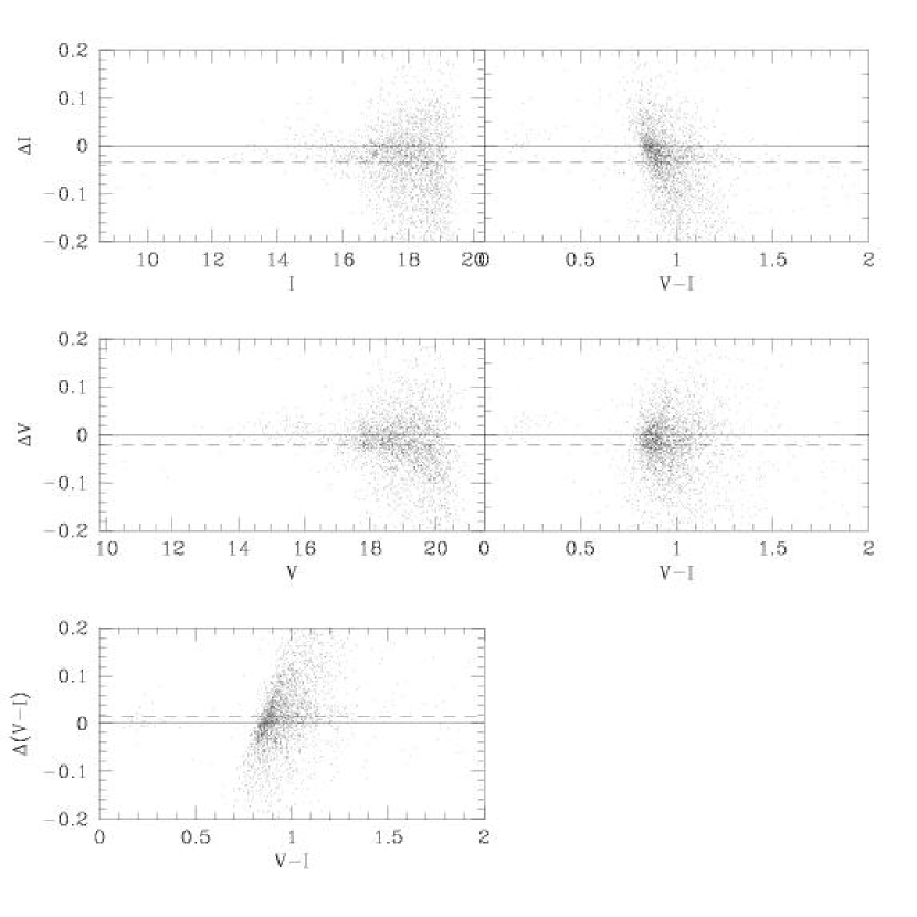
Figure 4: Residuals (in the sense ours minus theirs) from the star-by-star comparison of our photometry with that of Rosenberg et al. (2000). The dashed line represents the median value of all points.

Figure 18: Comparison of the observed and theoretical (BV) $V$ band luminosity function of M12. The metallicity has been chosen to fall within the range determined in $\S 4.1$, a value close to the CG value. A slightly younger model (12 Gyr), or correspondingly smaller distance modulus, shows better agreement with the SGB “jump”.

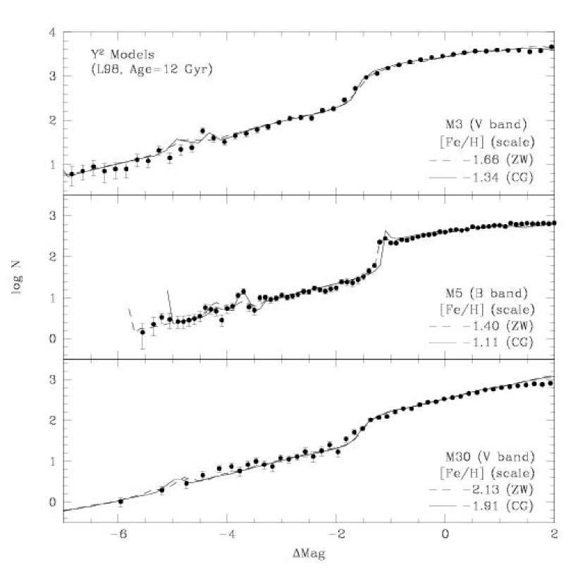
Figure 29: Comparison of the observed luminosity functions of M3 (top panel), M5 (middle panel), and M30 (bottom panel) with the Y² theoretical luminosity functions (using the L98 color-$T_{\mbox{eff}}$ transformation table). The magnitude scale has been shifted to match a common point on the upper main-sequence as discussed in $\S 6.2.1$.

Table 1: Median residuals for comparison samples

Comparison	$B$	$V$	$I$	($V-I$)	$(B-V)$	$N$
VB02	$\cdots$	$-0.056\pm 0.001$	$-0.063\pm 0.001$	$0.006\pm 0.002$	$\cdots$	$8731$
R00	$\cdots$	$-0.021\pm 0.003$	$-0.034\pm 0.003$	$0.015\pm 0.002$	$\cdots$	$2962$
B96	$-0.048\pm 0.011$	$-0.021\pm 0.008$	$\cdots$	$\cdots$	$-0.028\pm 0.006$	$1360$
S00	$-0.010\pm 0.009$	$-0.022\pm 0.005$	$\cdots$	$\cdots$	$0.009\pm 0.010$	$67$

Table 2: M12 [V,(B-V)] Fiducial Points

$V$	$(B-V)$	$N$
19.8758	0.7487	572
19.7758	0.7470	557
19.6758	0.7334	609
19.5758	0.7285	548
19.4758	0.7095	555
19.3758	0.6999	602
19.2758	0.6989	574
19.1758	0.6892	536
19.0758	0.6832	567
18.9758	0.6735	522

Note. — The complete version of this table is in the electronic edition of the Journal. The printed edition contains only a sample.

Table 3: M12 [V,(V-I)] Fiducial Points

$V$	$(V-I)$	$N$
20.2758	1.0705	371
20.1758	1.0502	419
20.0758	1.0322	529
19.9758	1.0180	534
19.8758	0.9978	572
19.7758	0.9800	557
19.6758	0.9700	609
19.5758	0.9478	548
19.4758	0.9352	555
19.3758	0.9227	602

Note. — The complete version of this table is in the electronic edition of the Journal. The printed edition contains only a sample.

Table 4: M12 [V,(V-I)] Fiducial Points from von Braun et al. (2002)

$V$	$(V-I)$	$N$
22.1750	1.5157	254
22.0250	1.4734	379
21.8750	1.4278	437
21.7250	1.3946	421
21.5750	1.3405	397
21.4250	1.3099	405
21.2750	1.2608	364
21.1250	1.2353	382
20.9750	1.1951	371
20.8250	1.1625	362

Note. — The complete version of this table is in the electronic edition of the Journal. The printed edition contains only a sample.

Table 5: Metal-Poor Subdwarfs with Well-Measured Parallaxes

HIC	HD/Gliese	$E(B-V)$	$V$	$\pi$ (mas)	$\sigma_{\pi}/\pi$	$M_{V}$	$\sigma_{M_{V}}$	$V\!-\!I$	[Fe/H]	$\delta(V-I)$	$(V-I)_{o}$
Subdwarfs Used in MS Fit
$38541$	$64090$	$0.000$	$8.276$	$35.29$	$0.029$	$6.01$	$0.06$	$0.771$	$-1.48$	$0.006$	$0.801$
$57939$	$103095$	$0.000$	$6.422$	$109.21$	$0.007$	$6.61$	$0.02$	$0.891$	$-1.24$	$-0.005$	$0.903$
$74234$	$134440$	$0.005$	$9.418$	$33.68$	$0.050$	$7.03$	$0.11$	$1.000$	$-1.28$	$0.014$	$1.018$
$74235$	$134439$	$0.005$	$9.052$	$34.14$	$0.040$	$6.70$	$0.08$	$0.913$	$-1.30$	$0.004$	$0.932$
$24316$	$34328$	$0.003$	$9.436$	$14.55$	$0.069$	$5.21$	$0.15$	$0.647$	$-1.44$	$-0.005$	$0.673$
$98020$	$188510$	$0.001$	$8.830$	$25.32$	$0.046$	$5.83$	$0.10$	$0.753$	$-1.37$	$0.009$	$0.774$
Subdwarfs Eliminated from MS Fit
$46120$	Gl 345	$0.012$	$10.089$	$16.46$	$0.060$	$6.14$	$0.13$	$0.728$	$-1.75$	$-0.042$	$0.774$
$70681$	$126681$	$-0.001$	$9.302$	$19.16$	$0.075$	$5.66$	$0.17$	$0.727$	$-0.90$	$-0.037$	$0.702$
$100568$	$193901$	$0.003$	$8.644$	$22.88$	$0.054$	$5.41$	$0.11$	$0.678$	$-1.00$	$-0.039$	$0.664$
$67655$	$120559$	$0.020$	$7.918$	$40.02$	$0.025$	$5.92$	$0.05$	$0.755$	$-0.95$	$-0.044$	$0.734$
$104659$	$201891$	$0.003$	$7.367$	$28.26$	$0.036$	$4.61$	$0.08$	$0.656$	$-0.97$	$0.016$	$0.638$
$100792$	$194598$	$0.003$	$8.335$	$17.94$	$0.069$	$4.56$	$0.15$	$0.629$	$-1.02$	$-0.002$	$0.616$
$18915$	$25329$	$0.000$	$8.502$	$54.14$	$0.020$	$7.17$	$0.04$	$1.007$	$-1.69$	$0.026$	$1.06$

Table 6: M12 $V$ Band Luminosity Function

$V$	log $N$	$\sigma_{high}$	$\sigma_{low}$
12.065	0.1388	0.2323	0.5333
12.515	0.1388	0.2323	0.5333
12.665	0.1387	0.2323	0.5333
12.815	0.1390	0.2323	0.5333
12.965	0.1385	0.2323	0.5333
13.115	0.4402	0.1761	0.3010
13.415	0.3151	0.1979	0.3740
13.565	0.4409	0.1761	0.3010
13.715	0.6160	0.1487	0.2279
13.865	0.3151	0.1979	0.3740

Note. — The complete version of this table is in the electronic edition of the Journal. The printed edition contains only a sample.

Table 7: M12 $I$ Band Luminosity Function

$I$	log $N$	$\sigma_{high}$	$\sigma_{low}$
10.125	-.1946	0.3011	1.0000
10.425	0.1065	0.2324	0.5338
10.725	-.1946	0.3010	1.0000
10.875	-.1946	0.3010	1.0000
11.025	0.5044	0.1606	0.2576
11.175	-.1946	0.3010	1.0000
11.325	0.2826	0.1980	0.3742
11.625	0.2826	0.1980	0.3741
11.775	0.2826	0.1980	0.3742
11.925	0.1065	0.2323	0.5334

Note. — The complete version of this table is in the electronic edition of the Journal. The printed edition contains only a sample.

Table 8: Input physics 

	$\alpha$-enhanced Models
Parameter	Y2	BV	Richard & VandenBerg
Solar mixture	GN93	AG89/G90,G91	GN93
Initial He abundance	$Y_{p}=0.233$	$Y_{p}=0.237$	$Y_{p}=0.237$
Reaction Rates	BP92	BP92	BP92
Equation of State	OPAL96 (R96)	see Appendix of V00	E73/CD92
Opacity	OPAL96 (RI95,IR96)	OPAL92 (RI92)	OPAL96
Low-Temperature Opacity	AF94	AF94	P94
$\alpha_{\textsc{{mlt}}}$	$1.74$	$1.89$	$1.69$
Gravitational Settling	He diffusion (T94)	none	Yes (see T98)
Radiative Acceleration	none	none	R98

References

- Alexander & Ferguson (1994) Alexander, D. R. & Ferguson, J. W. 1994, ApJ, 437, 879
- Anders & Grevesse (1989) Anders, E. & Grevesse, N. 1989, Geochim. Cosmochim. Acta, 53, 197
- Bahcall & Pinsonneault (1992) Bahcall, J. N., & Pinsonneault, M. H. 1992, Rev. Mod. Phys., 60, 297
- Bahcall et al. (1997) Bahcall, J. N., Pinsonneault, M. H., Basu, S., & Christensen-Dalsgaard, J. 1997, Phys. Rev. Lett., 78, 171
- Bennett et al. (2003) Bennett, C. L. et al. 2003, ApJS, 148, 1
- Bergbusch (1993) Bergbusch, P. A. 1993, AJ, 106, 1024
- Bergbusch (1996) Bergbusch, P. A. 1996, AJ, 112, 1061
- Bergbusch & VandenBerg (1992) Bergbusch, P. A. & VandenBerg, D. A. 1992, ApJS, 81, 163
- Bergbusch & VandenBerg (2001) Bergbusch, P. A. & VandenBerg, D. A. 2001, ApJ, 556, 322 (BV)
- Bolte (1994) Bolte, M. 1994, ApJ, 431, 223
- Brocato et al. (1996) Brocato, E., Buonanno, R., Malakhova, Y., & Piersimoni, A. M. 1996, A&A, 311, 778 (B96)
- Burgarella & Buat (1996) Burgarella, D. & Buat, V. 1996, A&A, 313, 129
- Carney et al. (1994) Carney, B. W., Latham, D. W., Laird, J. B., & Aguilar, L. A. 1994, AJ, 107, 2240
- Carretta & Gratton (1997) Carretta, E. & Gratton, R. G. 1997, A&AS, 121, 95 (CG)
- Carretta et al. (2000) Carretta, E., Gratton, R. G., Clementini, G., & Fusi Pecci, F. 2000, ApJ, 533, 215
- Chaboyer et al. (1992) Chaboyer, B., Deliyannis, C. P., Demarque, P., Pinsonneault, M. H., & Sarajedini, A. 1992, ApJ, 388, 372
- Chaboyer et al. (2001) Chaboyer, B., Fenton, W. H., Nelan, J. E., Patnaude, D. J., & Simon, F. E. 2001, ApJ, 562, 521
- Christensen-Dalsgaard, Gough, & Thompson (1992) Christensen-Dalsgaard, J., Gough, D. O., & Thompson, M. J. 1992, ApJ, 378, 413
- Christensen-Dalsgaard & Daeppen (1992) Christensen-Dalsgaard, J. & Daeppen, W. 1992, A&A Rev., 4, 267
- Dean (1981) Dean, J. F. 1981, Monthly Notes of the Astronomical Society of South Africa, 40, 14
- degl’Innocenti, Weiss, & Leone (1997) degl’Innocenti, S., Weiss, A., & Leone, L. 1997, A&A, 319, 487
- Eggleton, Faulkner, & Flannery (1973) Eggleton, P. P., Faulkner, J., & Flannery, B. P. 1973, A&A, 23, 325
- Faulkner & Swenson (1993) Faulkner, J. & Swenson, F. J. 1993, ApJ, 411, 200
- Ferraro et al. (1999) Ferraro, F. R., Messineo, M., Fusi Pecci, F., de Palo, M. A., Straniero, O., Chieffi, A., & Limongi, M. 1999, AJ, 118, 1738
- Gratton et al. (2003) Gratton, R. G., Bragaglia, A., Carretta, E., Clementini, G., Desidera, S., Grundahl, F., & Lucatello, S. 2003, A&A, 408, 529
- Green, Demarque, & King (1987) Green, E. M., Demarque, P., & King, C. R. 1987, The revised Yale isochrones and luminosity functions, New Haven: Yale Observatory, 1987.
- Grevesse & Noels (1993) Grevesse, N., & Noels, A. 1993, in Origin and Evolution of the Elements, ed. N. Prantzos, E. Vangioni-Flam, & M. Cassé (Cambridge: Cambridge Univ. Press), 14
- Grevesse et al. (1990) Grevesse, N., Lambert, D. L., Sauval, A. J., van Dishoeck, E. F., Farmer, C. B., & Norton, R. H. 1990, A&A, 232, 225
- Grevesse et al. (1991) Grevesse, N., Lambert, D. L., Sauval, A. J., van Dishoek, E. F., Farmer, C. B., & Norton, R. H. 1991, A&A, 242, 488
- Guhathakurta et al. (1998) Guhathakurta, P., Webster, Z. T., Yanny, B., Schneider, D. P., & Bahcall, J. N. 1998, AJ, 116, 1757
- Guenther & Demarque (1997) Guenther, D. B. & Demarque, P. 1997, ApJ, 484, 937
- Hanson (1979) Hanson, R. B. 1979, MNRAS, 186, 875
- Iben (1968) Iben, I. 1968, Nature, 220, 143
- Iglesias & Rogers (1996) Iglesias, C. A. & Rogers, F. J. 1996, ApJ, 464, 943
- Kim et al. (2002) Kim, Y., Demarque, P., Yi, S. K., & Alexander, D. R. 2002, ApJS, 143, 499 (Y2)
- Kraft & Ivans (2003) Kraft, R. P. & Ivans, I. I. 2003, PASP, 115, 143 (KI)
- Landolt (1992) Landolt, A. U. 1992, AJ, 104, 340
- Langer, Bolte, & Sandquist (2000) Langer, G. E., Bolte, M., & Sandquist, E. 2000, ApJ, 529, 936
- Lee, Demarque, & Zinn (1994) Lee, Y., Demarque, P., & Zinn, R. 1994, ApJ, 423, 248
- Lejeune, Cuisinier, & Buser (1998) Lejeune, T., Cuisinier, F., & Buser, R. 1998, A&AS, 130, 65
- Lucy (1974) Lucy, L. B. 1974, AJ, 79, 745
- Mandushev et al. (1996) Mandushev, G. I., Fahlman, G., Richer, H. B., & Thompson, I. B. 1996, AJ, 112, 1536
- Piotto et al. (2002) Piotto, G. et al. 2002, A&A, 391, 945
- Proffitt (1994) Proffitt, C. R. 1994, ApJ, 425, 849
- Proffitt & Vandenberg (1991) Proffitt, C. R. & Vandenberg, D. A. 1991, ApJS, 77, 473
- Racine (1971) Racine, R. 1971, AJ, 76, 331
- Reid et al. (2001) Reid, I. N., van Wyk, F.,Marang, F., Roberts, G., Kilkenny, D., & Mahoney, S. 2001, MNRAS, 325, 931
- Renzini & Fusi Pecci (1988) Renzini, A. & Fusi Pecci, F. 1988, ARA&A, 26, 199
- Richard et al. (1996) Richard, O., Vauclair, S., Charbonnel, C., & Dziembowski, W. A. 1996, A&A, 312, 1000
- Richard et al. (2002) Richard, O., Michaud, G., Richer, J., Turcotte, S., Turck-Chièze, S., & VandenBerg, D. A. 2002, ApJ, 568, 979
- Richer et al. (1998) Richer, J., Michaud, G., Rogers, F., Iglesias, C., Turcotte, S., & LeBlanc, F. 1998, ApJ, 492, 833
- Riello et al. (2003) Riello, M. et al. 2003, A&A, 410, 553
- Rogers & Iglesias (1992) Rogers, F. J. & Iglesias, C. A. 1992, ApJ, 401, 361
- Rogers & Iglesias (1995) Rogers, F. J. & Iglesias, C. A. 1995, in ASP Conf. Ser. 78: Astrophysical Applications of Powerful New Databases, ed. S. J. Adelman and W. L. Wiese (San Francisco: ASP), 31
- Rogers, Swenson, & Iglesias (1996) Rogers, F. J., Swenson, F. J., & Iglesias, C. A. 1996, ApJ, 456, 902
- Rood et al. (1999) Rood, R. T. et al. 1999, ApJ, 523, 752
- Rosenberg et al. (1999) Rosenberg, A., Saviane, I., Piotto, G., & Aparicio, A. 1999, AJ, 118, 2306
- Rosenberg et al. (2000) Rosenberg, A., Aparicio, A., Saviane, I., & Piotto, G. 2000, A&AS, 145, 451 (R00)
- Rutledge et al. (1997) Rutledge, G. A., Hesser, J. E., Stetson, P. B., Mateo, M., Simard, L., Bolte, M., Friel, E. D., & Copin, Y. 1997, PASP, 109, 883
- Rutledge, Hesser, & Stetson (1997) Rutledge, G. A., Hesser, J. E., & Stetson, P. B. 1997, PASP, 109, 907
- Ryan & Norris (1991) Ryan, S. G. & Norris, J. E. 1991, AJ, 101, 1835
- Ryan, Norris, & Beers (1999) Ryan, S. G., Norris, J. E., & Beers, T. C. 1999, ApJ, 523, 654
- Saad & Lee (2001) Saad, S. M. & Lee, S. 2001, Journal of Korean Astronomical Society, 34, 99
- Salaris & Weiss (2002) Salaris, M. & Weiss, A. 2002, A&A, 388, 492
- Sandquist et al. (1996) Sandquist, E. L., Bolte, M., Stetson, P. B., & Hesser, J. E. 1996, ApJ, 470, 910
- Sandquist et al. (1999) Sandquist, E. L., Bolte, M., Langer, G. E., Hesser, J. E., & Mendes de Oliveira, C. 1999, ApJ, 518, 262
- Sato, Richer, & Fahlman (1989) Sato, T., Richer, H. B., & Fahlman, G. G. 1989, AJ, 98, 1335
- Schlegel, Finkbeiner, & Davis (1998) Schlegel, D. J., Finkbeiner, D. P., & Davis, M. 1998, ApJ, 500, 525
- Schuster & Nissen (1989) Schuster, W. J. & Nissen, P. E. 1989, A&A, 221, 65
- Spergel et al. (2003) Spergel, D. N. et al. 2003, ApJS, 148, 175
- Spite & Spite (1982) Spite, F. & Spite, M. 1982, A&A, 115, 357
- Stetson (1987) Stetson, P. B. 1987,PASP,99, 191
- Stetson (1990) Stetson, P. B. 1990, PASP, 102, 932
- Stetson (1991) Stetson, P. B. 1991, in ASP Conf. Ser. 13: The Formation and Evolution of Star Clusters, ed. K. Janes, (San Francisco: ASP), 88
- Stetson (1992) Stetson, P. B. 1992, JRASC, 86, 71
- Stetson (1994) Stetson, P. B. 1994, PASP, 106, 250
- Stetson (2000) Stetson, P. B. 2000, PASP, 112, 925
- Stetson & Harris (1988) Stetson, P. B. & Harris, W. E. 1988, AJ, 96, 909
- Straniero, Chieffi, & Limongi (1997) Straniero, O., Chieffi, A., & Limongi, M. 1997, ApJ, 490, 425
- Suntzeff et al. (1993) Suntzeff, N. B., Mateo, M., Terndrup, D. M., Olszewski, E. W., Geisler, D., & Weller, W. 1993, ApJ, 418, 208
- Thomas (1967) Thomas, H.-C. 1967, Zeitschrift fur Astrophysics, 67, 420
- Thoul, Bahcall, & Loeb (1994) Thoul, A. A., Bahcall, J. N., & Loeb, A. 1994, ApJ, 421, 828
- Turcotte et al. (1998) Turcotte, S., Richer, J., Michaud, G., Iglesias, C. A., & Rogers, F. J. 1998, ApJ, 504, 539
- VandenBerg (2000) VandenBerg, D. A. 2000, ApJS, 129, 315
- Vandenberg, Larson, & de Propris (1998) Vandenberg, D. A., Larson, A. M., & de Propris, R. 1998, PASP, 110, 98
- VandenBerg et al. (2000) VandenBerg, D. A., Swenson, F. J., Rogers, F. J., Iglesias, C. A., & Alexander, D. R. 2000, ApJ, 532, 430
- VandenBerg et al. (2002) VandenBerg, D. A., Richard, O., Michaud, G., & Richer, J. 2002, ApJ, 571, 487
- VandenBerg & Clem (2003) VandenBerg, D. A. & Clem, J. L. 2003, AJ, 126, 778
- von Braun et al. (2002) von Braun, K., Mateo, M., Chiboucas, K., Athey, A., & Hurley-Keller, D. 2002, AJ, 124, 2067 (VB02)
- Zinn (1985) Zinn, R. 1985, ApJ, 293, 424
- Zinn & West (1984) Zinn, R. & West, M. J. 1984, ApJS, 55, 45 (ZW)
- Zoccali & Piotto (2000) Zoccali, M. & Piotto, G. 2000, A&A, 358, 943