A SCUBA Map in the Spitzer First Look Survey: Source Catalog and Number Counts

Abstract

Using the SCUBA instrument on the JCMT, we have made a submillimeter mosaic at 850$\mu$m of a subarea of the Spitzer First Look Survey (FLS). Our image covers the central 151 arcmin² of the northern extragalactic Continuous Viewing Zone (CVZ) field of the FLS to a median 3$\sigma$ depth of 9.7 mJy. The image contains ten 850$\mu$m sources detected at 3.5$\sigma$ or higher significance, of which five are detected at $\geq$4$\sigma$. We make the catalog of these SCUBA-selected FLS sources available to the community. After correcting for incompleteness and flux bias, we find that the density of sources brighter that 10mJy in our field is (1.3${}^{+1.1}_{-0.7}$)$\times$$10^{2}$ deg^-2 (95% Poisson confidence limits), which is consistent with other surveys that probe the bright end of the submillimeter population.

1. INTRODUCTION

Launched in the second half of 2003, the Spitzer Space Telescope (formerly SIRTF), the fourth and final of NASA’s Great Observatories, holds the promise of addressing many outstanding questions related to dust-enshrouded galaxy formation at high redshift. One of the first science observations to be undertaken by Spitzer is the Spitzer First Look Survey (FLS), a first look at the mid-IR sky at sensitivities that are two orders of magnitude deeper than previous large-area surveys. In addition to Spitzer data at 3.6, 4.5, 5.8, 8.0, 24, 70, and 160$\mu$m, the FLS has also been observed in deep ground-based campaigns at optical (KPNO 4m to $R$=25.5, 5$\sigma$ in a 2″ aperture) and radio (VLA to 115$\mu$Jy, 5$\sigma$, per 5″ beam at 1.4GHz; Condon et al. 2003) wavelengths. The Spitzer FLS data will be released to the public in early 2004 and, together with the deep ancillary ground-based data, will provide the community with the first systematic look at the properties of faint Spitzer-selected extragalactic sources.

While Spitzer will discover many dust-enshrouded high-$z$ objects and will greatly help us understand their nature, the fact that it does not image at wavelengths longward of 160$\mu$m presents some important limitations. For example, for typical dust temperatures (20–40K; e.g., Dunne et al. 2000), the longest Spitzer passband barely probes longward of the peak of the thermal dust emission for galaxies at even moderate redshifts, making it difficult to estimate their bolometric luminosities and hence infer quantities such as dust masses and star formation rates. Moreover, with increasing redshift (or decreasing dust temperature), an object’s dust emission peak shifts redward of the longest Spitzer wavelength, causing strong negative k-corrections and making a galaxy at high redshift (or one with low dust temperatures) fade rapidly out of a Spitzer-selected sample.

In this Letter we present complementary long-wavelength imaging observations of a section of the Spitzer FLS, obtained at 850$\mu$m with the Submillimetre Common User Bolometer Array (SCUBA) on the James Clerk Maxwell Telescope (JCMT). In a future paper we will discuss in detail the multiwavelength properties of sources in the area of our SCUBA map; the purpose of the present Letter is to quickly make available to the community the source catalog of objects from our SCUBA observations within the public-release Spitzer FLS.

2. THE DATA

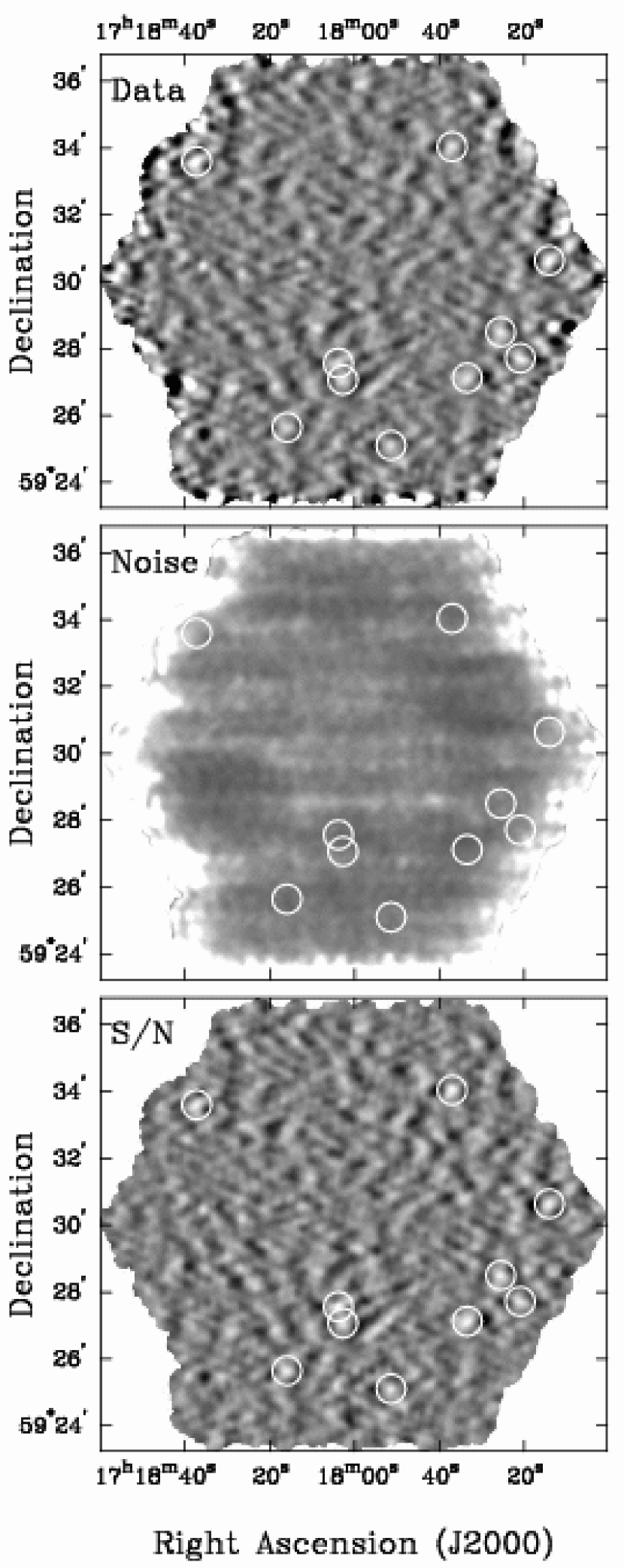
Figure 1.— The beam-convolved signal (top), noise (middle), and RMS signal-to-noise (bottom) maps of our 850$\mu$m survey. These maps are mosaics of multiple individual SCUBA pointings. Sources detected at $>$3.5$\sigma$ are marked with circles. A HIGH QUALITY VERSION OF THIS FIGURE CAN BE OBTAINED FROM THE AUTHORS.

2.1. Observations

We used the SCUBA instrument (Holland et al. 1999) on the JCMT to observe a contiguous area of 151 arcmin² centered on the nominal center of the FLS northern extragalactic CVZ field at R.A.=17:18:00, Dec=+52:24:30 (J2000.0). SCUBA is an array of 37 bolometers at 850$\mu$m and 91 at 450$\mu$m that is able to observe simultaneously at both wavelengths, although particularly excellent weather is required for 450$\mu$m observations. In its jiggle-map mode — which is the mode we used — a SCUBA observation has a footprint of $\sim$2′ diameter; to cover a large contiguous area we tiled our field in a spiral pattern on a hexagonal grid, starting at the nominal central FLS coordinates. A typical point in our combined map received a total of 2048 seconds of integration, split into 4 visits that were separated in time by many hours and, often, nights.

The data were obtained during thirteen nights from 2002 March through 2003 March, using a total of 7.5 usable (out of 10 allocated) shifts of JCMT time. The weather varied from grade 1 to grade 4, or ${\tau}_{850}\sim$ 0.1 to ${\tau}_{850}\sim$ 0.45, where ${\tau}_{850}$ is a measure of the optical depth at 850$\mu$m. To remove the rapidly-varying sub-mm sky we used the standard SCUBA chopping technique with a chop-throw of 30″ held constant in RA. This technique produces the familiar negative-positive-negative beam pattern apparent in many SCUBA maps and can be used to increase the significance of detection for individual sources by taking advantage of the signal in the off-beams.

Throughout the observing campaign sky opacity was measured using skydip observations every $\sim$1.5 hours, though less often in exceptionally transparent and stable weather. Pointing checks were performed every 1.5 hours and the data were flux calibrated using standard JCMT flux calibrators.

Table 1 850$\mu m$ sources detected at $>$3.5$\sigma$.                       

ID	RA(2000)	Dec(2000)	S850(mJy)	S/N
FLS850.1803+2733	17:18:03.9	+59:27:33	10.9$\pm$2.4	4.5
FLS850.1736+3401	17:17:36.9	+59:34:01	11.3$\pm$2.6	4.4
FLS850.1733+2706	17:17:33.5	+59:27:06	11.0$\pm$2.6	4.3
FLS850.1725+2828	17:17:25.6	+59:28:28	12.3$\pm$3.0	4.2
FLS850.1837+3335	17:18:37.3	+59:33:35	16.0$\pm$4.0	4.0
FLS850.1714+3036	17:17:14.1	+59:30:36	14.6$\pm$3.7	3.9
FLS850.1816+2538	17:18:16.0	+59:25:38	9.5$\pm$2.4	3.9
FLS850.1751+2505	17:17:51.5	+59:25:05	10.5$\pm$2.8	3.8
FLS850.1721+2741	17:17:21.0	+59:27:41	13.5$\pm$3.7	3.7
FLS850.1802+2703	17:18:02.8	+59:27:03	10.7$\pm$2.9	3.7

2.2. Data reduction

The data were reduced using the standard SCUBA User Reduction Facility (SURF) procedure. After removing the nod, the data were flatfielded and corrected for sky opacity using the skydip measurements. At each second the mean sky level was subtracted from the array and noise spikes were iteratively removed from the bolometer timestreams. Finally, the data were rebinned onto the sky plane to produce the final (unsmoothed) map.

To increase the sensitivity to point sources, the unsmoothed map was convolved with a template beam profile that was made from observations of point-like calibration sources and contains the negative-positive-negative beam pattern. This technique reduces the frequency of spurious sources which do not convolve well with the beam, and increases the S/N by incorporating the flux from the two off-source positions into the final flux measurements. The top panel of Figure 1 shows our beam-convolved map.

We used the method of Eales et al. (2000) to estimate the noise across our map. We produced Monte Carlo simulations of each raw bolometer time stream using the same noise level as in the real data but adding no signal. These simulated data were then reduced using the same set of steps as the real data resulting in a simulated sky map. We produced 500 such simulated sky maps and the noise at each pixel in the data map, shown in the middle panel of Figure 1, is taken to be the variance between these 500 simulations at that pixel. The noise level determined by this method agrees well with the noise estimated from the real data map. The median noise value is 3.2 mJy (1$\sigma$) and the spatial distribution of the noise level is quite uniform across the entire field except near its edges.

2.3. Source detection and the object catalog

We used a combination of the data and noise maps to perform an automated source search. A S/N map (bottom panel of Figure 1) was produced by dividing the beam-convolved data map by the beam-convolved noise map; all peaks with S/N$\geq$3.5 in this S/N map are source candidates. To make the source finding procedure objective and automated (a must for our completeness simulations in § 3), the actual search is performed using the SExtractor source-detection software (Arnouts & Bertin, 1996) on a truncated version of the S/N map. Specifically, to restrict SExtractor to sources with S/N$\geq$3 and to suppress confusion due to the negative off-beams of bright sources, we set all values S/N$<$3 to zero before running SExtractor. As confirmed by visual inspection, this technique reliably finds all the peaks above S/N$>$3. There are 27 peaks with S/N$>$3, and 10 with S/N$>$3.5.

Figure 2.— The cumulative 850$\mu$m number counts. The filled circle shows the results from the present work in the Spitzer FLS. Error bars are 95% Poisson confidence limits. Following Borys et al. (2003), overlaid are two predictions based on representative galaxy evolution models from Rowan-Robinson (2001) — the dashed line is for a universe with ($\Omega_{M},\Omega_{\Lambda}$)=(1.0, 0.0), and the dotted line is for ($\Omega_{M},\Omega_{\Lambda}$)=(0.3, 0.7).

Tables 1 presents all sources detected with S/N$>$3.5. Column 1 gives the source ID, columns 2 and 3 give the coordinates of the source determined by SExtractor in the truncated S/N map, column 4 gives the source flux, and column 5 lists the significance of the detection.

Based on Gaussian noise statistics we expect that at S/N=3.5 we should have $\sim$1 spurious source in our map (the number of expected spurious sources is close to zero at S/N=4). Contamination by spurious sources does not have a large effect on the sub-mm source counts we discuss in the following section (§ 3), but we mention it here to caution the reader that, statistically, $\sim$1 of the sources in Table 1 may not be real.

3. SOURCE COUNTS

To date, two surveys have targeted the bright end ($S_{850\mu m}$$\gtrsim$10mJy) of the sub-mm population and both show a steep slope of the cumulative source counts. Scott et al. (2002) surveyed two spatially independent fields with a total area of 260 arcmin², while Borys et al. (2002, 2003) studied an area of 165 arcmin² in the region of the northern Hubble Deep Field. Both surveys show strong qualitative clustering of sources which may skew their source count results. Here, we use our 151 arcmin² FLS SCUBA map to make a third, independent measurement of the submillimeter source counts at the bright end of the population.

Table 2 850$\mu m$ number counts in the Spitzer FLS

$S_{850}$(mJy)	$n_{objects}$	raw $N(>S)$	corrected $N(>S)$
10	9	215 ${}^{+194}_{-112}$	133 ${}^{+112}_{-69}$
12	4	95 ${}^{+148}_{-69}$	54 ${}^{+92}_{-39}$
14	2	48 ${}^{+125}_{-42}$	29 ${}^{+76}_{-26}$

Our raw cumulative source counts are presented in column 3 of Table 2, where we have counted all objects detected at S/N$>$3.5. However, we are interested in sources that are close to the noise level and so, to properly calculate the source density, we must account for two effects: incompleteness and flux bias. Clearly, the number counts of faint sources near the detection threshold will suffer from incompleteness, making it necessary to correct their observed numbers upwards. Additionally, however, detected sources will also have suffered from flux boosting: while sources whose flux densities are scattered below the detection threshold are not counted in the sample, those that are scattered into the sample from below the detection threshold will necessarily have their flux densities overestimated. These two effects compete against each other, but for a source population where numbers increase quickly with decreasing true flux density (as is the case here) flux boosting should dominate.

We studied these issues using Monte Carlo simulations that implant artificial sources into our data and seek to recover them using the same technique that we used for constructing our source catalog in § 2.3. We generated artificial sources by flux-scaling the empirical beam map constructed from observations of bright point-source flux calibrators. An artificial source was then added at a random (but known) location to the data map, the resulting map was divided by the noise map to form the S/N map, and then the object-finding and flux measurement procedures used on the real data were applied to search for the artificial object. To statistically assess the completeness and flux bias properties of our map, this procedure was repeated, one artificial object at a time, for a range of input fluxes and spatial positions.

This Monte Carlo procedure applied to our SCUBA map results in a matrix, $S_{true,obs}$, that gives the probability that, for a source of a known input flux density $S_{true}$, we will recover an object of an observed flux density $S_{obs}$. To understand the incompleteness and flux bias effects on the population of sources, we need to consider their effects on a plausible true source count distribution. Following Borys et al. (2003) we assume the following functional form to describe the underlying source count population:

$$\frac{dN(>S)}{dS}\propto\left[\left(\frac{S}{S_{0}}\right)^{\alpha}+\left(\frac{S}{S_{0}}\right)^{\beta}\right]^{-1};$$ (1)

we adopt $S_{0}$=1.8mJy, $\alpha$=1, $\beta$=3.3 (Scott et al. 2002), although varying these parameters within reasonable ranges ($S_{0}$=0.5–5, $\alpha$=0.5–2, $\beta$=2–4) does not drastically affect our results. We then multiply the assumed source count model of Equation 1 by the transform matrix $S_{true,obs}$ to obtain the “observed” source counts. The ratios of the integrated source counts in the underlying source count model to those “observed” by our procedure, give us the correction factors that need to be applied to the raw source counts in Table 2 to correct for incompleteness and flux bias.

The corrected integrated source counts are given in Column 4 of Table 2 and are plotted in Figure 2 together with counts from other surveys. Our 850$\mu$m FLS source counts are clearly in agreement with both the results of the 8mJy survey of Scott et al. (2002) and with the HDF data of Borys et al. (2003) and we conclude that, at least on the basis of source number densities, there is no evidence that our FLS subfield is not representative of the sub-mm galaxy population.

4. SUMMARY AND DISCUSSION

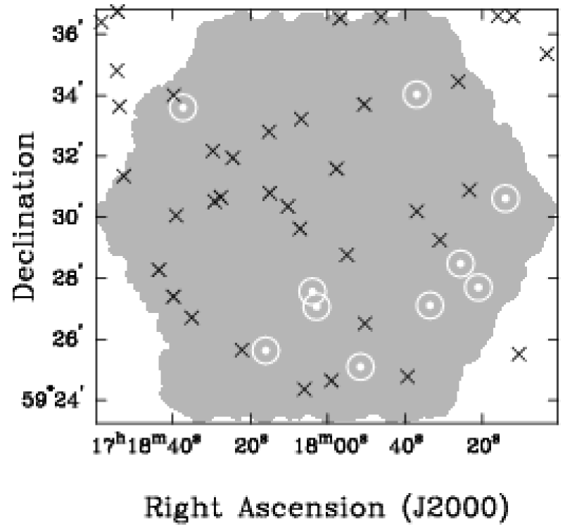
Figure 3.— Positions of VLA radio detections compared to our 850$\mu$m SCUBA sources. Radio detections are shown as crosses, while SCUBA sources are represented with white circled points, with the size of the inner point corresponding roughly to the 15″ diameter of the SCUBA beam. None of our SCUBA sources have radio detections. A HIGH QUALITY VERISION OF THIS FIGURE CAN BE OBTAINED FROM THE AUTHORS

In this Letter we presented our SCUBA observations of a 151 arcmin² subarea in the northern CVZ field of the Spitzer First Look Survey. We found a total of 10 sources at S/N$>$3.5 and make their particulars available to the community. Our integrated source counts are consistent with those of the other two surveys of the bright end of the sub-mm population, namely the 8mJy Survey (Scott et al. 2002) and the Hubble Deep Field supermap (Borys et al. 2002, 2003). Given that extragalactic sub-mm sources cluster strongly on the scales of current surveys (see, e.g., Figure 1), the fact that our number counts agree with those of the other two surveys gives an important confirmation of the numbers of SCUBA sources at the bright end of the population. Equally significantly, the agreement between our number counts and those of other surveys suggests that the subfield of the FLS that we imaged is not unrepresentative of the extragalactic sky.

We will study the multi-wavelength properties of the sub-mm sources in our map once the Spitzer FLS data are released, In the meantime, we have compared the positions of our SCUBA detections with those of objects in the 1.4GHz VLA map of the FLS (Condon et al. 2003). There is no correspondence between the radio-selected and the sub-mm selected populations (see Figure 3) down to the limit of the VLA catalog (115 mJy, 5$\sigma$). This lack of radio detection of any of our sub-mm sources can be used to constrain their redshifts (Dunne, Clements & Eales 2000; see also Yun & Carilli, 2002): given the VLA flux limit and the rather narrow dynamic range of these data, most of our sub-mm sources appear to be at $z$$\gtrsim$ 1.6–1.7 and the brightest two at $z$ $\gtrsim$ 2.0, (however, these results are likely to be affected by flux boosting). These redshift constrains are in line with our current knowledge of the redshift distribution of sub-mm selected sources: the median redshift of the population is believed to lie at $z\sim$ 2–3, and evidence exists of a flux-redshift relation, such that more luminous sub-mm selected systems (such as those in our survey) reside at higher redshifts than the less luminous objects (Ivison et al. 2002, Smail et al. 2002, Webb et al. 2003, Chapman et al. 2003, Clements et al. 2004). The lack of 1.4 GHz detection of our sub-mm sources is thus not unexpected: deeper radio data will be needed to detect and identify these systems. We will explore these issues further once the Spitzer FLS data are released.

We thank the Joint Astronomy Centre staff who helped us obtain these data, and our colleagues who carried out some of these observations through the Canadian flexible scheduling scheme. We also thank Colin Borys for providing in digital format the number counts shown in Fig. 2. The JCMT is operated by the Joint Astronomy Centre on behalf of the Particle Physics and Astronoy Reseach Council of the United Kingdom, the Netherlands Organisation for Scientific Research, and the National Research Council of Canada.

References

- (1) Bertin, E. & Arnouts, S. 1996, A&AS, 117, 393
- Borys et al. (2002) Borys, C., Chapman, S.C., Halpern, M., & Scott, D. 2002, MNRAS, 330, L63
- Borys et al. (2003) Borys, C., Chapman, S., Halpern, M., & Scott, D. 2003, MNRAS, 344, 385
- Chapman et al. (2002) Chapman, S.C., Scott, D., Borys, C., & Fahlman, G. 2002, MNRAS, 330, 92
- Chapman et al. (2003) Chapman, S.C., Blain, A.W., Ivison, R.J., & Smail, I.R. 2003 Nature, 422, 695
- Clemente et al. (2004) Clements, D., et al. 2004, MNRAS, in press (astro-ph/0312269)
- Condon et al. (2003) Condon, J.J. et al. 2003, AJ, 125, 2411
- Dunne et al. (2000) Dunne, L., Eales, S., Edmunds, M., Ivison, R., Alexander, P., & Clements, D.L. 2000 MNRAS, 315, 115
- Eales et al. (2000) Eales, S., Lilly, S., Webb, T., Dunne, L., Gear, W., Clements. D., & Yun, M. 2000, AJ, 120, 2244
- Holland et al. (1999) Holland, W.S. et al. 1999, MNRAS, 303, 659
- Hughes et al. (1998) Hughes, D.H., et al. 1998, Nature, 394,241
- Ivison et al. (2002) Ivison, R.J., et al. 2002, MNRAS, 337, 1
- Rowan-Robinson (2001) Rowan-Robinson, M. 2001, ApJ, 549, 745
- Scott et al. (2002) Scott, S.E., et al. 2002, MNRAS, 331, 817
- Smail et al. (2002) Smail, I., Ivison, R.J., Blain, A.W., Kneib, J.-P. 2002, MNRAS, 331, 495
- Webb et al. (2003) Webb, T.M.A., Lilly, S.J., Clements, D.L., Eales, S., Yun, M., Brodwin, M., Dunne, L., & Gear, W. K. 2003, ApJ, 597, 680
- Yun & Carilli (2002) Yun, M.S. & Carilli, C.L. 2002, ApJ, 568 ,88