HST STIS Ultraviolet Spectral Evidence of Outflow in Extreme Narrow-line Seyfert 1 Galaxies: I. Data and Analysisl^,

Abstract

We present HST STIS observations of two extreme NLS1s, IRAS 13224$-$3809 and 1H 0707$-$495. The spectra are characterized by very blue continua, broad, strongly blueshifted high-ionization lines (including C IV and N V), and narrow, symmetric intermediate- (including C III], Si III], Al III) and low-ionization (e.g., Mg II) lines centered at their rest wavelengths. The emission-line profiles suggest that the high-ionization lines are produced in a wind, and the intermediate- and low-ionization lines are produced in low-velocity gas associated with the accretion disk or base of the wind. In this paper, we present the analysis of the spectra from these two objects; in a companion paper we present photoionization analysis and a toy dynamical model for the wind. The highly asymmetric profile of C IV suggests that it is dominated by emission from the wind, so we develop a template for the wind from the C IV line. We model the bright emission lines in the spectra using a combination of this template, and a narrow, symmetric line centered at the rest wavelength. We also analyzed a comparison sample of HST spectra from 14 additional NLS1s, and construct a correlation matrix of emission line and continuum properties. A number of strong correlations were observed, including several involving the asymmetry of the C IV line.

1 Introduction

In 1992, it was demonstrated by Boroson & Green that the optical emission line properties in the region of the spectrum around H$\beta$ are strongly correlated with one another. A principal components analysis allowed the largest differences among optical emission line properties to be gathered together in a construct commonly known as “Eigenvector 1”. The strongest differences hinged on the strength of the Fe II and [O III] emission, and the width and asymmetry of H$\beta$. This set of strong correlations is remarkable, as it involves correlations among the dynamics and gas properties between emission regions separated by vast distances. Furthermore, the same set of correlations are observed in samples selected in many different ways. This pervasiveness leads us to believe that we are observing the manifestation of a primary physical parameter. A favored explanation is that it is the accretion rate relative to the black hole mass onto the active nucleus (e.g., Boller, Brandt & Fink 1996; Pounds, Done & Osborne 1995; Comastri et al. 1998; Leighly 1999ab; Mathur 2000; Mineshige et al. 2000; Kuraszkiewicz et al. 2000; Pounds et al. 2001; Puchnarewicz et al. 2001; Ballantyne, Iwasawa, & Fabian 2001; Boroson 2002; Crenshaw, Kraemer & Gable 2003).

Narrow-line Seyfert 1 galaxies (NLS1s) are identified by their optical emission line properties. They typically have narrow permitted optical lines (FWHM of H$\beta<2000\rm\,km\,s^{-1}$), weak forbidden lines ([O III]/H$\beta<3$; this distinguishes them from Seyfert 2 galaxies), and frequently they show strong Fe II emission (Osterbrock & Pogge 1985; Goodrich 1989). These are the same properties that define the Boroson & Green (1992) Eigenvector 1, and indeed, NLS1s fall at one end of Eigenvector 1. Thus, the study of NLS1s offers an attractive research opportunity: if we can understand the origin of the emission-line properties of NLS1s, then we may be in a position to understand AGN emission in general. Furthermore, because as least some of the lines in NLS1s are narrow, identification of the frequently strongly-blended lines is less ambiguous than it is in broad-line objects.

NLS1 research dramatically increased after the publication of a seminal paper in 1996 by Boller, Brandt & Fink describing their discovery that NLS1s have systematically steeper ROSAT spectra than AGN with broad optical lines. Subsequently it was shown from ASCA observations that the hard X-ray spectrum is also steeper (Brandt, Mathur & Elvis 1997; Leighly 1999b), and that the X-ray emission shows higher fractional amplitude of variability (Leighly 1999a). These results were generally interpreted as evidence that the black hole is systematically smaller in NLS1s, implying a higher accretion rate relative to the Eddington value compared with Seyfert 1 galaxies with broad optical lines.

Once the high accretion rate paradigm was established, it could be used to understand why NLS1s have narrow optical lines. Boller, Brandt, & Fink (1996) mention that if the black hole mass in NLS1s is smaller, and the emission lines are produced at the same radius as in broad-line objects (due to the same radiating flux) the dynamical velocities will be smaller, and narrower lines will be produced. This theme was expanded upon by Wandel & Boller (1998), who consider the fact that the steeper soft X-ray spectrum of NLS1s, when extrapolated into the UV, implies a larger ionizing flux relative to their luminosity. This causes the emission region to be larger where the velocities are smaller.

However, the optical emission lines are only one side of the coin; UV emission lines, generally characterized by a higher degree of ionization, may also provide valuable information. This is because the optical and UV emission lines are generally not produced in the same gas. The best evidence for this comes from so-called reverberation mapping experiments (e.g., Peterson 1993). Also, the profiles of the emission lines suggest this as well, as the higher ionization lines are observed to be generally broader than the lower ionization lines (e.g., Baldwin 1997). Therefore, we may learn more about NLS1s by studying their UV emission lines.

Several groups have investigated the UV emission line properties of NLS1s. The first paper investigating a sample of IUE spectra from NLS1s was published by Rodríguez-Pascual, Mas-Hesse & Santos-Lleó (1997). They reported that the strongest UV emission lines have broad wings, unlike the optical emission lines, and they speculate that the UV line-emitting gas may be optically thin in the continuum.

Kuraszkiewicz et al. (2000) present a detailed study of IUE and HST spectra from NLS1s. They found that, compared with broad-line quasars, the equivalent widths of C IV and Mg II are low. They found that, in the cases where the lines could be deblended, the Si III]/C III] ratio was high. In addition, the Si IV+O IV] feature near 1400 Å was found to be strong compared with C IV, and the Al III equivalent width was high. They also found that although the UV emission lines in NLS1s are broader than the Balmer lines, they still tend to be narrower than those lines in broad-line quasars. They then model many of the emission line ratios using a 1-zone Cloudy model (Ferland 2001). They infer that the line ratios imply that the ionization parameter is lower and the density is higher in NLS1s than in broad-line Seyfert 1 galaxies. We comment on their inferences in the companion paper to this one (Leighly 2004a; hereafter referred to as Paper II).

Wills et al. (1999), studying the HST spectra from a small sample of PG quasars, found that Eigenvector 1 is also associated with a high Si III] to C III] ratio, stronger UV low-ionization lines, weaker C IV, but stronger N V. They infer from these spectra that NLS1s are typified by high densities, low ionization parameters, and nitrogen enhancement, perhaps from nuclear starbursts.

All the work done so far on the UV spectra of NLS1s has been generally confined to studies of the properties of the integrated lines, to a greater or lesser extent, depending on the analysis. Specifically, the conditions of a single-zone BLR are modelled or discussed more or less quantitatively, and evidence for a radially-extended BLR is inferred when particular lines are found to not be consistent with the one-zone model (e.g., Kuraszkiewicz et al. (2000) infer that, since the observed Mg II is underpredicted by the one-zone model, it must be produced in a different region than the other UV emission lines). However, we know that generally the emission line profiles are not all the same, and higher ionization lines tend to have broader profiles. This implies that the gas properties are different among regions with larger or smaller line-of-sight velocities, and therefore a study of the average properties could be misleading.

In this paper, we present the observations and analysis of HST observations of two NLS1s that have truly remarkable UV spectra. In Section 2, we introduce the targets, describe our observations and discuss the analysis of the emission lines. In Section 3, we compare the results from these two NLS1s with spectra from 14 NLS1s drawn from the HST archive, and perform a correlation analysis and a principal components analysis on the results. In a companion paper II, photoionization analysis, and a toy dynamical model are presented, and the results are discussed. Partial results from this study have been published previously in Leighly (2000) and Leighly (2001). We use $H_{0}=50\rm\,km\,s^{-1}\,Mpc^{-1}$ and $q_{0}=0.5$ unless otherwise noted.

2 Observations and Analysis

2.1 The Targets

We observed two NLS1s, IRAS 13224$-$3809 (z=0.066, V=15.9) and 1H 0707$-$495 (z=0.040, V=15.7), using HST STIS during 1999. Groundbased optical spectra were also obtained. The observing log is given in Table 1.

These two NLS1s are quite remarkable objects and can be considered to be extreme for their class in terms of their X-ray properties. They showed among the largest fractional amplitudes of variability in a sample of NLS1s observed by ASCA (Leighly 1999a). ROSAT monitoring observations of IRAS 13224–3809 found strong soft X-ray flaring by up to a factor of 60 in as short time interval as two days (Boller et al. 1997). Large amplitude X-ray variability was also reported during a long ASCA observation (Dewangen et al. 2002). Their X-ray spectra are also unusual. They show extremely strong X-ray soft excess components and lie on the extreme of the variability–soft excess correlation (Leighly 1999b; Leighly 2004b). XMM–Newton observations of 1H 0707$-$495 and IRAS 13224$-$3809 reveal a peculiar deep absorption feature near 7 keV that is quite difficult to explain (Boller et al. 2002; Boller et al. 2003). The XMM-Newton observation of 1H 0707$-$495 showed primarily color-independent X-ray variability (Boller et al. 2002). In contrast, a Chandra observation of 1H 0707$-$495 found strong spectral variability in that the soft X-rays varied much less than the hard X-rays (Leighly et al. 2002; Leighly et al. in prep.).

The motivation for the HST observations was the discovery of a peculiar feature near 1 keV observed in the ASCA spectra (Leighly et al. 1997). This feature appeared to be an absorption edge, but the energy was clearly too high to be ascribed to highly-ionized oxygen, which is generally the most important source of X-ray opacity. Leighly et al. (1997) speculated that oxygen was indeed responsible for the feature, and, if so, the absorbing gas was outflowing at rather large velocities. This interpretation was strengthened by the similarity between luminous NLS1s and low-ionization BALQSOs (e.g., Boroson & Meyers 1992 for I Zw 1). Reasoning that X-ray absorption may be accompanied by UV absorption, we proposed to make use of the much superior spectral resolution (relative to ASCA CCDs) provided by HST STIS, and look for evidence for outflowing gas in the UV. We note here that no evidence for absorption intrinsic to the quasars was found in the spectra. This result leaves the issue of the X-ray features unresolved, since it is certainly plausible that the X-ray absorption lines could be produced in gas too highly ionized to present opacity in the UV. We also note that subsequent high resolution X-ray observations using Chandra reveal absorption lines (Leighly et al. 2002; Leighly et al. in prep.)

2.2 The HST observations and Continua

Our observations were made during the first cycle that the STIS spectrometer was available. We made the HST observations using a “pattern” in order to decrease possible systematic error due to fixed pattern noise. Three or four steps along the slit were used for each spectroscopic element. The relative wavelength calibration of each spectrum was checked prior to summing the spectra by cross correlating with a preliminary average spectrum. Many Galactic absorption lines were observed in the spectra. These were used to identify and correct zero-point wavelength offsets in the spectra. Then, the redshift was obtained from the optical and UV spectra. In the optical spectrum of IRAS 13224$-$3809, H$\beta$ is extended in the spatial direction. The extended emission probably originates in a starburst in the host galaxy, and therefore provides a good estimate of the systemic redshift. The extended emission contributes to the narrowest part of the H$\beta$ profile; therefore, we estimated the redshift from centroid of the top of the H$\beta$ line. Interestingly, O III has a blue offset of $370\rm\,km\,s^{-1}$ (Grupe & Leighly 2002), similar to I Zw 1 (Phillips et al. 1976). The redshift of 1H 0707$-$495 was estimated also using the centroid of the top of the H$\beta$ line. These redshifts were consistent with that inferred from Mg II, if that line is centered at the rest wavelength, and the centroid of the narrow part of Ly$\alpha$. The measured redshifts were 0.066 and 0.040 for IRAS 13224$-$3809 and 1H 0707$-$495, respectively.

The UV spectra are displayed in Fig. 1 along with nonsimultaneous optical spectra obtained at CTIO (details in Table 1) and a composite quasar spectrum from the LBQS (Francis et al. 1991) for comparison. This figure shows that IRAS 13224$-$3809 and 1H 0707$-$495 have continua as blue as the average quasar. This result is in agreement with the discovery by Grupe et al. (1998) that soft X-ray selected AGN from the ROSAT All Sky Survey, a sample which is comprised of 1/2 NLS1s, generally have quite blue optical–UV continuum spectra; some are as blue as predicted by the standard (thin) accretion disk model ($F_{\nu}\propto\nu^{1/3}$; $F_{\lambda}\propto\lambda^{-7/3}$). For comparison, a line with a slope of $-7/3$ is included on Fig. 1 (which is plotted in terms of $F_{\lambda}$), as well as one also with slope $-0.32$, which is the median slope in the LBQS (Francis et al. 1991). Very blue optical spectra seem to be common among luminous NLS1s (see also RGB J0044+193: Siebert et al.  1999; RX J0134.2$-$4258: Grupe et al. 2000; RX J2217.9$-$5941: Grupe, Thomas & Leighly 2001; PHL 1811: Leighly et al. 2001).

The optical spectrum from 1H 0707$-$495 appears to be slightly offset in normalization from the UV spectra. This offset could be due to aperture effects, or from variability, as there was a one-year interval between the optical and UV spectra. However, the continuum slopes in the UV and optical spectra appear to be consistent. In contrast, the optical spectrum from IRAS 13224$-$3809 appears to be much flatter than the UV continuum spectrum. This object is an extremely luminous far-infrared source (Norris et al. 1990), and we suspect that the flattening is due to contamination of the central engine emission by the starburst. We suspect that similar contamination was present in other spectra from this object, leading to reports that the optical–UV continuum spectrum is flat (e.g., Boller et al. 1993). The UV spectra presented here show that the central engine continuum spectrum is not flat, but very clearly blue.

2.3 The Emission Lines and Modeling

The spectra are shown in more detail in Fig. 2. In this plot, we follow Laor et al. (1997) and mark the rest wavelengths of many of the strong lines frequently observed in AGN spectra. Our identification of the emission features are discussed below.

These spectra are characterized by the following properties:

• Strong Fe II emission. Emission lines from Fe III are also identified. The Fe II is strong enough that it forms a pseudocontinuum makes identification of the real continuum difficult, but it can also be identified as a forest of relatively narrow lines, especially near 2000 Å.

• Broad and blueshifted high-ionization lines. The high-ionization lines, including Ly$\alpha$, N V, the Si IV–O IV] complex, and C IV are all relatively broad (FWHM are approximately 5000$\,\rm km\,s^{-1}$) and blueshifted, with little emission redward of the rest wavelength, at least in C IV and N V.

• Relatively narrow intermediate- and low-ionization lines centered at the rest wavelength. C III], Si III] and Mg II are narrow (900–1900$\rm\,km\,s^{-1}$), and their profiles are reflection-symmetric about about the rest wavelength.

• Strong lower ionization lines, including Si II and C II.

The spectra most strongly resemble that of the NLS1 prototype I Zw 1, which also shows blueshifted high-ionization lines, narrow intermediate- and low-ionization lines and strong Fe II and Fe III (Laor et al. 1997). However, as discussed in Section 3, they are somewhat different than the other narrow-line Seyfert 1 galaxies and quasars. The presence of strong low-ionization lines in our spectra is similar to that seen in several PG quasars (Wills et al. 1999; see their Figure 1).

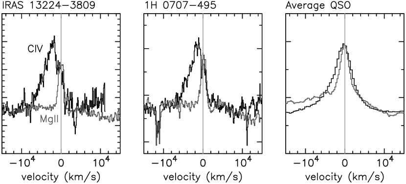
Figure 3: The rescaled representative high-ionization line C IV superimposed on the representative low-ionization line Mg II as a function of velocity, for our two NLS1s and the average quasar (Francis et al. 1991). The average quasar high-ionization line is slightly broader and slightly blueshifted compared with the low-ionization line. In contrast, the low-ionization lines in NLS1s are much narrower and the high-ionization lines are strongly blueshifted.

The profound differences in the profiles of the high- and low-ionization lines are highlighted in Fig. 3, which compares the profile of the prototypical high-ionization line C IV with the profile of a low-ionization line Mg II, for our NLS1s and for a composite quasar spectrum (Francis et al. 1991). It has been previously noted that high-ionization lines are frequently broader and strongly blueshifted compared with the low-ionization lines (e.g., Tytler & Fan 1992; Marziani et al. 1996). The velocity offsets in C IV described by Marziani et al. (1996) range from zero to $\sim 3000$; the centroids of our profiles are offset by $\sim 2500\rm\,km\,s^{-1}$, as large as the largest values values found by Marziani et al. These profiles are most simply explained if the high-ionization line-emitting gas is accelerated toward us in a wind, while the low-ionization line-emitting gas is located on the surface of the accretion disk, or in the low-velocity base of the wind. The wind may be accelerated by radiative-line driving from the strong UV continuum. This process is commonly inferred to be occurring in hot stars and cataclysmic variables, but it has also been applied to AGN (e.g., Murray et al. 1995; Murray & Chiang 1998; Proga, Stone, & Kallman 2000), and we discuss this further in Paper II. The accretion disk is assumed optically thick, so that we do not see the receding wind on the other side. Hence, the emission lines are predominantly blueshifted. Collin-Souffrin et al. (1988) were the first to suggest a two-component broad-line region in which the high-ionization lines are produced in a wind, and the low-ionization lines are associated with the outer parts of the accretion disk. The spectra presented here arguably provide the strongest support for this scenario to date.

Because the high-ionization lines are nearly disjoint in velocity space compared with the low- and intermediate-ionization lines, we model them separately. We then use the results to constrain photoionization models for the conditions of the disk and wind separately in Paper II. Such an undertaking is fraught with peril. In the emission-line profile, we observe only the velocity component parallel to our line of sight. Especially problematic is the gas at zero velocity, as the emitting matter may have huge transverse velocity that we cannot detect. However, such an approach is not without precedent: Baldwin et al. (1996) analyzed the spectra from a luminous quasar Q0207$-$398 in this way.

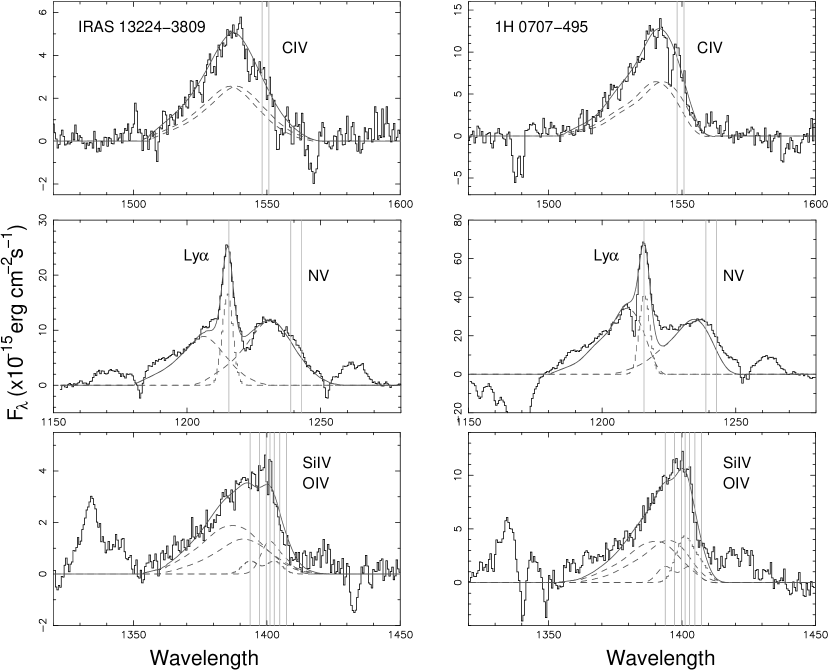
Figure 4: Line models for the C IV region, the Ly$\alpha$/N V region, and the Si IV/O IV] region. The dark grey dashed lines show the components and the light grey vertical lines show the positions of the lines in the rest frame. Resonance lines were assumed to be optically thick and thus their ratios were assumed to be 1:1. O IV] was assumed to be optically thin (see text).

To measure the line properties, we adopted a modified version of the procedure used by Baldwin et al. (1996). We outline the procedure here, and describe the application to each region of the spectra below; the results are given in Fig. 4 and Table 2. First, we make several simplifying assumptions. Fig. 3 suggests that, to zeroth order, the wind and disk lines are kinematically disjoint. We further assume, to begin with, that all high-ionization lines have the same velocity profile; we comment on the validity of that assumption below. Then, since C IV is isolated compared with the other high-ionization lines, we use it to create a wind-profile template that is used to model the other high-ionization lines. The procedure used to develop the template is described in the next section.

The intermediate- and low-ionization lines appear to be predominately symmetric about their rest wavelengths; therefore, we model them using symmetric Lorenzian or Gaussian profiles. Preliminary examination of spectra showed that we could not assume the same velocity width for all the intermediate- and low-ionization lines, as Mg II could be seen to be clearly significantly narrower than C III]. Therefore, in fitting the intermediate- and low-ionization lines, we allowed the width to remain an adjustable parameter so long as it could be constrained usefully in the fitting. Generally, the widths could be usefully constrained unless the lines are very weak (e.g., Section 2.3.7), or unless the feature is comprised of several heavily-blended components, in which case we fixed the velocity width for particular individual lines to the values measured from other lines.

The next sections explain the process that we used to model the spectra. Throughout, we use a locally-defined continuum. This is necessary because the strong Fe II and Fe III multiplets that may form a pseudo-continuum that masks the real continuum. We note that placement of the continuum is a potentially significant source of uncertainty in the measurement of the emission-line flux.

2.3.1 The C IV region

First, the continuum was locally identified around the C IV emission line, then fit with a linear model and subtracted. Next, we removed the portions of the profile contaminated by absorption lines originating in our Galaxy (Blades et al. 1988). The Galactic column is significant in the direction of our quasars, and there are a number of fairly strong lines apparent in the spectrum. Careful examination of the C IV profile reveals faint absorption lines that were detected by Blades et al. but were not identified. The regions of the profile contaminated by absorption lines were removed and the profile was fitted with a high-order spline model.

The C IV line is a doublet, but the final template should consist of the contribution of only one component. To derive the profile of one component, we used a procedure similar to that used by Baldwin et al. 1996. We assumed that each of the two components contributed equally to the line (that is, the line is optically thick). The approximate contribution of one component of the doublet was then obtained from the spline model by a sort of bootstrap method. The doublet components are separated by 4–5 wavelength bins. Therefore, the 4 or 5 points at longer wavelength side of the spline model consists solely of the lower energy component, so these can be used to determine the amplitude of the 4 or 5 longest wavelength points of the template. Points shortward of this consist of the sum of both lower-energy and the higher-energy components. At the next point, where $i=6$, for example, the amplitude of the higher-energy component at $i$ is already known, because it must have the amplitude of the lower energy component at $i=$1–2. Then, since the sum of the lower and higher-energy components at any point $i$ must equal the spline model at that point, the amplitude of lower-energy profile at point $i$ can be solved for. Thus, the amplitudes of the remaining points could be determined iteratively. The C IV emission lines, the contribution of each multiplet and the resulting profiles are shown in Fig. 4. Interestingly, the shape of the template is slightly but distinguishably different between the two objects.

2.3.2 The Ly$\alpha$ and N V region

The template developed using the C IV profile, shown in Fig. 4, was next fit to the Ly$\alpha$/N V region in both spectra. A second-order polynomial was used to model the local continuum, which was then subtracted. The fitting was done by first transforming the template spectrum to the rest energy of the emission line in question and then adjusting the normalization until some part of the profile did not obviously exceed the height of the spectrum; i.e., if the model were subtracted from the data, no obvious negative residuals would be present. A narrow component of Ly$\alpha$ was also clearly visible. This is inferred to originate from the disk, and it is modelled as a Gaussian. Both components of the N V doublet were modeled and the flux ratio between the doublet components was again assumed to be 1 to 1. The results are shown in Fig. 4.

This procedure resulted in a good fit for IRAS 13224$-$3809. Excess emission shortward of Ly$\alpha$ may come from C III* $\lambda 1176$ line, a line that has been identified in the spectrum of the prototype NLS1 I Zw 1 (Laor et al. 1997). Si II is strong elsewhere in the spectrum and may contribute near 1190 Angstroms as well. Note that the deficit near 1222 Å in the rest frame is caused by Galactic absorption (Fig. 2).

The fit results for 1H 0707$-$495 are less satisfactory. Excess emission is present both redward and blueward of the N V line. The blueward emission could also be present in IRAS 13224$-$3809 but it may be hidden by the Galactic absorption line near 1222 Å. This excess emission could be an indication that our assumption that all of the resonance lines have the same profile is to some degree incorrect; however, we cannot clearly see the blue side of that line because it is blended with the broad Ly$\alpha$ line, so we cannot clearly evaluate whether this assumption is good or not. We plan to address this question in a future paper involving the O VI line observed in the FUSE spectrum of 1H 0707$-$495.

In both cases, since the wind profile fits N V well, we conclude there is no disk contribution to this line. Both a disk and a wind component are necessary, on the other hand, to model Ly$\alpha$.

2.3.3 The Si IV/O IV] region

The feature near 1400Å is clearly broad and asymmetric and at least part of it must be emitted in the wind. This is a complicated feature in AGN in general, because it may be comprised of emission from both O IV] and Si IV. Si IV is usually a lower-ionization line than the other lines produced in the wind. The disk contributes low-ionization lines (e.g., Mg II, as in Fig. 3); therefore it is possible that there is a contribution from Si IV from the disk in the 1400 Å feature. To try to account for this possibility in a general way, our model for this region consists of components of wind emission from each of Si IV and O IV] that are modelled using the template developed from C IV as discussed in Section 2.3.1. We also include components of disk emission from each of Si IV and O IV] that are modelled as Gaussians, as discussed above. There are thus 4 components in the model.

We assumed that the emission ratios of the two components of the Si IV doublet have equal flux (optically thick). For O IV] we assumed optically thin ratios. These depend partially on density and were found to be 0.011:0.225:0.458:0.082:0.225 for the $\lambda$1397.2, $\lambda$1399.8, $\lambda$1401.2, $\lambda$1404.8 & $\lambda$1407.4 emission lines respectively (Flower & Nussbaumer (1975) and Nussbaumer & Storey (1982) assuming a density of $10^{9}\rm\,cm^{-3}$.

We first determined the upper limits of the four components listed above by overlaying each one on the line profile separately and adjusting the amplitude until some part of the component was as large as the line; i.e., no large negative fit residuals were permitted. Those upper limits are listed in Table 2.

Next, we investigated whether or not the entire feature could have been emitted in the wind; that is, is the disk component necessary? We overlayed the sum of the O IV] and Si IV wind components on the profile, adjusting the amplitudes as described above. While the shortest wavelength, blueshifted part of the feature could be modeled by the sum of the wind components from O IV] and Si IV, the longest wavelength part, near the rest energies of O IV] and Si IV, could not. We inferred that the excess emission near the rest energies of these features is emission from the disk. To model the disk component, emission line blends for Si IV and O IV] were constructed using Gaussians, assuming again that Si IV is optically thick and O IV] is optically thin, as above. The widths of these Gaussians could not be independently determined in the fit, so we assumed a FWHM of 7 Angstroms, corresponding to $1500\,\rm km\,s^{-1}$. This is close to the value found for the 1900 Å lines (Section 2.3.4).

The 1400 Å feature is very complicated. We show a model in Fig. 4 that appears to fit the profile, and the parameters for this model are listed in the Table 2; however, we do not claim that this model is unique. All we can really conclude is that emission from both the disk and the wind is necessary to explain the profile; the wind portion is needed to explain the shorter wavelength, blueshifted part, and the disk portion is needed to explain the rest-wavelength part. But we really cannot tell how much of each component originates in each of Si IV and O IV]. The photoionization modelling presented in Paper II is helpful for understanding this feature.

Adjacent to the 1400Å feature, there is excess emission near 1420 Å that could be another emission line. A possible candidate could be S IV] $\lambda\lambda$ 1416.93, 1423.86 (Harper et al. 1999).

2.3.4 The Al III/C III]/Si III] region

In the wavelength range between 1800 and 2000 Å, we expect to find emission from C III], Si III] and Al III, as well as possibly Fe III and Fe II. Identification of the continuum in this region is very difficult because of the strong Fe II and Fe III lines. In IRAS 13224$-$3809 we clearly identify fairly strong contributions from C III], Si III] and Al III. These lines appear to be narrow, symmetric, strongly peaked, and centered at the emission line wavelength. Thus, we infer they are from the disk and that no measurable wind component is present in the 1900Å feature. We use the spectral fitting package LINER (Pogge & Owen 1993) to model the lines. We first attempt to model the emission lines as Gaussians; however, they are too strongly peaked for this to provide a good fit. Therefore, we use Lorenzian profiles and obtain a better fit, although we note that Lorenzian profiles may overestimate the line flux due to the large contributions in the wings that are difficult to distinguish from the continuum. However, there remains excess emission around 1925 Å that most probably originates in the Fe III 34 multiplet. This multiplet consist of three lines at 1895.46, 1914.06, and 1926.30 Å (e.g., Graham, Clowes & Campusano 1996). We include these three emission lines in the model, assuming that their fluxes are equal (e.g., Hartig & Baldwin 1986; see also Section 3). In the final model, we hold the emission line wavelength fixed at the rest wavelength, the width of C III], Si III] and Al III are constrained to be equal, and the widths of the Fe III 34 multiplet components are constrained to be equal.

The spectrum from 1H 0707$-$495 appears to be more difficult to model well. There seems to be more Fe III present in the spectrum of this object. A completely satisfactory fit could not be obtained.

2.3.5 He II

This line was very difficult to identify and measure. Following the example of I Zw 1, and the other high ionization lines, we expected it to be strongly blueshifted and broad; i.e., from the wind. Indeed, we see no evidence for a narrow emission line at 1640 Å. We defined a local continuum from apparently line-free region, and measured the line using the wind template developed from the C IV profile, as was done above. This measurement is not very satisfactory as there are other emission features of the same amplitude, probably originating in Fe II, near the feature that we identify as He II.

2.3.6 Mg II region

The spectrum around Mg II is contaminated by broad humps of Fe II emission. This makes measurement of the flux and width of Mg II difficult. Following several other authors (e.g., Corbin & Boroson 1996; Dietrich et al. 2002), we develop an Fe II template from the medium-resolution HST spectrum from I Zw 1 following the procedure used by Vestergaard & Wilkes (2001). We adjust the amplitude of the Fe II template so that it fits the Fe II feature in the spectra. We then subtract the Fe II component, and fit the Mg II line using the LINER package. It turns out we cannot constrain the doublet ratio as was done for I Zw 1 (Laor et al. 1997), so we require the doublet component fluxes to be equal. We cannot distinguish between Gaussian and Lorenzian line profiles; however, we note that these lines are significantly narrower than C III] and Si III].

2.3.7 Other low-ionization lines

The fluxes of several weak low-ionization lines were required for photoionization modeling of the disk component in Paper 2. All of the lines considered in this section appeared to be centered at the rest wavelength, and symmetric, so we infer that they are entirely produced in the disk. They are sufficiently weak that we could only measure their flux with any confidence; their widths appear to be consistent with the other low-ionization lines. The C II lines at 1335Å and 2327Å were modeled using Gaussians, employing LINER to do the fitting. C II$\,\lambda 1335$Å was slightly blended with an unidentified line at 1345Å (also seen in I Zw 1; see Laor et al. 1997) so these two lines were modelled simultaneously. This procedure worked well for IRAS 13224$-$3809. 1H 0707$-$495 posed a more difficult case, as there were several strong absorption lines cutting through the C II$\,\lambda 1335$Å lines. The C II$\,\lambda 2327$Å was more difficult to model in both cases. It appeared to be perched on a broad, blended Fe II feature, and blended with Fe III. We were able to measure it with some confidence for IRAS 13224$-$3809, but did not obtain a measurement for 1H 0707$-$495. We also measured the flux and equivalent width of N III]$\lambda 1750$Å. This was difficult, as it is barely detectable in IRAS 13224$-$3809, so this measurement should be considered to be nearly an upper limit. It was more clearly detected in 1H 0707$-$495, and we measure the flux and equivalent width by defining the local continuum on both sides of the feature and integrating over the small excess at 1750Å.

2.3.8 H$\beta$ region

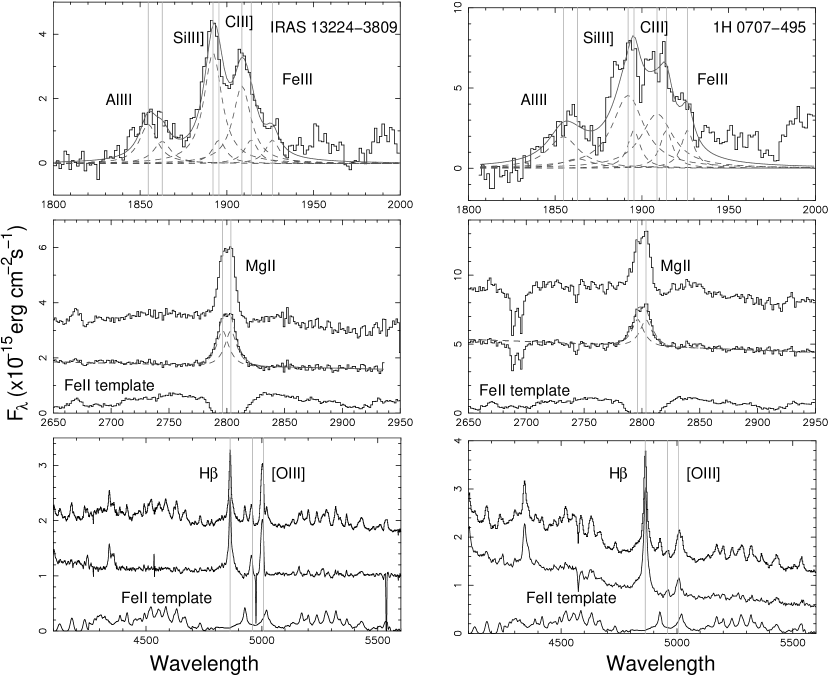
Figure 5: Line models for the Al III/Si III]/C III] region, the Mg II region, and the H$\beta$/[O III] region. The dark grey dashed lines show the components and the light grey vertical lines show the positions of the lines in the rest frame.

We also obtained groundbased optical spectra from these two objects. Near H$\beta$, the spectra in Narrow-line Seyfert 1 galaxies is frequently cluttered with multiplets of Fe II that make it difficult to measure the properties of H$\beta$ and [O III]. This problem is overcome by subtraction of an Fe II template developed from a high signal-to-noise spectrum from the prototype NLS1 I Zw 1 (e.g., Boroson & Green 1992). The Fe II subtracted spectra are displayed in Fig. 5. The H$\beta$ line was fitted with a Lorenzian profile to obtain the width.

2.3.9 Comparison with Composite Spectra

In Table 2, along with the emission-line measurements from IRAS 13224$+$3809 and 1H 0707$-$495, we list measurements of emission lines from three composite spectra: the LBQS composite (Francis et al. 1991); the radio-quiet composite from HST spectra (Zheng et al. 1997); a composite spectrum from the FIRST Bright Quasar Survey (Brotherton et al. 2001). In all cases, the equivalent widths of the prominent features in our spectra are the same or smaller than the equivalent widths in the composites, except for N V, which has larger equivalent widths in our spectra. Zheng et al. attempt to deconvolve N V from Ly$\alpha$; in that case, Ly$\alpha$ in our spectra are about one third, and N V are nearly double the equivalent width of that in the Zheng composite. The whole 1400Å feature and 1900Å feature have about the same equivalent width as the composite. Zheng et al. (1997) attempt a deconvolution of the 1900Å feature; our spectra have the same Al III equivalent widths, larger by a factor of two Si III] equivalent widths, and much smaller (by a factor of 3) C III] equivalent widths than the Zheng composite. The largest differences are in C IV and Mg II, which have much smaller (one fifth to one half) the equivalent width of the composite spectra. These comparisons underline the fact that the UV emission lines, excepting N V, are relatively weak in NLS1s.

3 Comparison with Other NLS1s

The UV and optical properties of IRAS 13224$-$3809 and 1H 0707$-$495, including their luminosity, their emission line profiles, and their equivalent widths and ratios, are almost identical. How do their properties compare with those of other NLS1s? This is an important question for two reasons. First, their X-ray properties, while again virtually identical to one another, are markedly different from those of other NLS1s. In a study of the X-ray properties of NLS1s using ASCA data, Leighly (1999b) found that there is a correlation between the prominence or strength of the soft excess and the amplitude of the variability, with IRAS 13224$-$3809 and 1H 0707$-$495 displaying among the strongest soft excesses and highest-amplitude variability in the sample. Also, these objects are two of the three that possess an unusual spectral feature near 1 keV that has been interpreted as highly blueshifted absorption feature (Leighly et al. 1997) or as strong Fe-L absorption (Nicastro, Fiore & Matt 1999). We would like to know if the differences between IRAS 13224$-$3809 and 1H 0707$-$495 and other NLS1s that are found in the X-ray band are also seen in the UV band. The second reason we are motivated to compare these two objects with other NLS1s involves our interpretation of our analysis of the UV spectra that is discussed in detail in Paper II.

To address these questions, we retrieved the spectra from a heterogeneous group of 14 NLS1s from the HST archive, and analyzed them. Analysis of properties of NLS1 UV spectra has been previously presented by several groups. However, reanalysis is necessary because we wish to investigate both the emission line profiles and their equivalent widths and ratios. The most detailed investigation to date was presented by Kuraszkiewicz et al. (2000). Our analysis differs from theirs in that they confined their analysis to the emission-line fluxes and ratios, while we are interested also in the emission-line profiles, in particular that of C IV, as well. A comparison of the blueshift of C IV with the width of H$\beta$ has been published by Marziani et al. (1996). However, they do not consider the fluxes and ratios of other important lines in the spectrum.

The following objects, listed in order of right ascension, were investigated: Mrk 335, WPVS 007, I Zw 1, Ton S180, RX J0134.2$-$4258, PG 1001$+$054, RE 1034$+$39, PG 1115$+$407, PG 1211$+$143, PG 1404$+$226, PG 1402$+$261, Mrk 478, Mrk 493, and Ark 564. These objects represent a range of redshifts from 0.024 to 0.235, and span two orders of magnitude in monochromatic luminosity at 2500Å; the luminosities of IRAS 13224$-$3809 and 1H 0707$-$495 are in the middle of the sample. Almost all of these spectra were obtained using the FOS detector and therefore we reprocessed all of them, using the Post Operational Archives (POA) calibration when appropriate. Ton S180 was observed with the STIS detector, and we retrieved those data from the archive using “on-the-fly” reprocessing.

We checked the wavelength calibration of each spectrum using the Galactic absorption lines. The spectra were then shifted up to $\sim 1.5$Å as necessary. Our first estimate of the redshift was obtained from the spectra directly, by fitting the Mg II lines. We assume that Mg II lines are centered at the systemic redshift. This is justified by the similarity between Mg II and H$\beta$ emission in AGNs (McLure & Jarvis 2002), and the fact that all of these objects have narrow H$\beta$ and Mg II. These redshifts were in good agreement with those listed in NED. The spectra were then shifted into the rest frame. The Galactic E(B-V) was obtained from NED, and the spectra were corrected using the CCM reddening law (Cardelli, Clayton & Mathis 1989).

We used a procedure similar to that employed for IRAS 13224$-$3809 and 1H 0707$-$495 as described in Section 3.1 to investigate the profile of the C IV line. We first identified and subtracted the local continuum, and excluded portions of the profile modified by Galactic absorption lines. We require a smoothed profile to study the shape of the line. We used two different methods depending on the signal-to-noise ratio to obtain the smoothed profile. When the signal-to-noise ratio was relatively high, we fit the continuum-subtracted spectrum in the region of the emission line with a spline function as described in Section 2.3.1. When the signal to noise is lower, the multinode spline could not be constrained, so instead we fit the profile with several Gaussians or Lorenzians, and used the model as our smoothed profile. In a few objects (Ark 564, WPVS 007, PG 1404+226), the line profiles were altered by the presence of strong associated absorption lines. For these objects, the line profiles were reconstructed using multiple-component fits, but there is no doubt that the result is uncertain, especially with regard to the equivalent widths. Therefore, these objects are denoted by a different symbol in plots that include C IV information. A broad absorption line is observed in PG 1001+054 (Brandt, Laor & Wills 2000). However, this broad absorption line appears to be sufficiently detached that it does not alter the C IV line profile.

We then measured a number of properties from the resulting C IV profile, including the flux and equivalent width. We investigated several possible ways to parameterize the shape and offset of the C IV line. We considered using the velocity offset (e.g., Marziani et al. 1996); however, this does not take into account the fact that the lines are very asymmetric. We looked into using the moments of the line profile (mean, variance, skew and kurtosis). We also investigated using the fraction of the line blueward of the rest wavelength (here taken to be 1549.5 Å, the average of the doublet wavelengths). We found that the mean wavelength is strongly correlated with the fraction of the emission blueward of 1549.5 Å, and finally opted to use the latter as the parameter representing the asymmetry and blueshift of the line. We also obtained the kurtosis as a measurement of the peakiness of the line: a line with positive kurtosis is pointy, and a line with negative kurtosis has a flattened profile.

Other high ionization lines were measured. We obtained a rough estimate of the flux and equivalent width of N V by modeling it with several Gaussians or Lorenzians. In some objects, the lines were narrow enough that N V could be cleanly separated from Ly$\alpha$, and the principal uncertainty in the measurements of the flux and equivalent width is the placement of the continuum. In other objects, N V overlapped Ly$\alpha$; we estimate the uncertainty in the flux and equivalent width may be as high as 40% for these objects. As discussed in Section 2.3.3 , the O IV] and Si IV lines near 1400Å were quite difficult to separate in IRAS 13224$-$3809 and 1H 0707$-$495. Thus, for these other objects, we measure the flux and equivalent width of the whole 1400Å feature by simply integrating over it after defining a local continuum. He II was also measured. In some objects, this line was blended with O III]$\lambda\lambda 1660.8,1666.1$; in these cases, we used a model consisting of several Gaussians to isolate the contribution of He II. In several objects, a significant source of uncertainty was determination of the continuum when the relatively weak He II line was blueshifted and broad. Finally, we computed ratios of the fluxes of the high-ionization lines with that of C IV.

The feature near 1900Å is comprised primarily of the intermediate ionization lines Al III, Si III], C III], and Fe III UV34. This was modeled in a way similar to that described in Section 2.3.4. As discussed in Vestergaard & Wilkes (2001), the Fe III UV34 multiplet (1894.8Å, 1914.1Å, 1926.3Å; ${}^{7}S-^{7}P^{\circ}$) contributes significant uncertainty to line measurements in this region. However, in all of the objects that we looked at, the intermediate ionization lines appeared to be narrow, symmetric, and centered at their rest wavelengths. We therefore assumed that all of the lines in the 1900Å feature have the same width, and assumed that they are centered at their rest wavelength. The presence of Fe III UV34 generally could be ascertained by the presence of the 1926Å line, which was discernible from the wings of C III] lines in these narrow-line objects. The gf values obtained from The Atomic Line list indicate that in the optically-thin case, the line ratios 1926:1914:1895 should be 1:1.4:1.8. However, radiative transfer is likely to be important for these lines. In some cases, the spectra were fit well assuming that the three Fe III lines have equal intensity, as would be appropriate if the gas is very optically thick. However, in several objects (e.g., Ark 564; Fig. 15), the 1914Å component was much stronger than the other two; this enhancement was discussed previously by Vestergaard & Wilkes (2000) for I Zw 1, although these authors do not give an explanation for it. It turns out that the upper-level energy for this transition is $82333.92\rm cm^{-1}$, corresponding to 1214.6Å, which is just 1.1Å from Ly$\alpha$. Therefore, the 1914Å component of the Fe III UV34 feature is plausibly selectively excited by Ly$\alpha$. Interestingly, this seems to be almost the only line emitted under broad-line region conditions that can be excited from the ground state by Ly$\alpha$; many more lines, including O I$\lambda 1302$ for example, may be pumped by Ly$\beta$, and Fe II may be pumped by Ly$\alpha$ from low-lying metastable levels (e.g., Sigut & Pradhan 2003). Therefore, we also fit with a model in which the 1895 and 1926 Å components are constrained to have equal intensities, and the 1914 Å intensity is left free. In this case, the 1914 Å component ranges from 1.8 to typically 3 times the strength of the other two. The fluxes of Al III, Si III], and C III] lines, and the velocity width of C III] were measured, and the ratios of Al III and Si III] to C III] were formed. The 1900Å feature is complex; thus, there is significant uncertainty in the relative intensities of the Si III] and C III] lines; Al III was separated sufficiently from the the other two that uncertainty in this line was dominated by the continuum placement.

We obtained the equivalent widths and velocity widths of the Mg II line after subtracting the UV Fe II as described in Section 2.3.6. A by-product of the Fe II subtraction procedure is a measure of the slope of the continuum $\alpha_{u}$, where $F(\lambda)\propto\lambda^{\alpha_{u}}$, in the UV between about 2200Å and 3050Å (see Moore & Leighly, in prep. for details). We also measured the monochromatic luminosity at restframe 2500Å and 1400Å. Finally, we used generally nonsimultaneous X-ray data to estimate $\alpha_{ox}$, the point-to-point power-law energy index between 2500Å and 2 keV in the rest frame. If available, ASCA data were used because flux at 2 keV could be estimated better than from ROSAT data in which 2 keV falls at the end of the bandpass. Uncertainties in intrinsic $\alpha_{ox}$ originate in the lack of simultaneity of the observations, and reddening or absorption arising in the host galaxy or AGN.

3.1 Correlations and Principle Components Analysis

We performed a correlation analysis of the parameters discussed above, using the Spearman rank correlation coefficient. In a few cases, parameters could not be measured: an example is RX J0134.2$-$4258, in which no C III], Si III] and Al III were detected. We also do not use the velocity width of C III] for 1H 0707$-$495 because it was much larger than the widths of other similar lines in that object (see Section 2.3.4). Since we are only missing one object (three in one case) among 16, we do not use a survival analysis. The probabilities of accidental correlation are given in the correlation matrix in Table 3.

We performed a principle components analysis using the correlation matrix. Although the number of objects and parameters is small, we obtain a fairly significant clustering of correlations. The first three eigenvectors are given in Table 4; they represent 78% of the variance in the sample. We caution that our sample is small, so these eigenvectors may not survive if faced with a larger sample. Nevertheless, they provide a convenient organizational framework in which to discuss the correlations.

3.1.1 Eigenvector 1: the C IV and other high-ionization line properties

Eigenvector 1 is aligned along the mutually strong correlations between C IV equivalent width and profile shape. A number of other parameters are strongly correlated or anticorrelated with the asymmetry of the C IV line. These include the high-ionization properties of the equivalent width of He II and the N V/C IV ratio, the intermediate-ionization line properties of the Al III/C III] ratio and the Si III]/C III] ratio, and the continuum property $\alpha_{ox}$. A number of these are shown in Fig. 7. Another interesting correlation is the one between the N V/C IV ratio and the Al III/C III ratio; we defer that discussion until Section 3.1.3.

The C IV asymmetry parameter is strongly anticorrelated with the C IV equivalent width; that is, the strongly blueshifted lines have the lowest equivalent width. This was previously reported in Leighly 2001 for this sample, and has since then been recovered from the SDSS quasars (Richards et al. 2002), and a similar correlation was previously noted by Wills et al. (1993). The kurtosis is strongly anticorrelated with the asymmetry parameter, implying that the more strongly blueshifted lines have a flattened rather than peaked profile. This result suggests the hypothesis that the narrow, symmetrical part of C IV is an additional component that increases the equivalent width of the whole line when present, as well as reducing the cumulative offset from the rest wavelength.

To test this idea, we constructed a composite line consisting of the wind profile from IRAS 13224$-$3809, and a narrow and symmetric line that has a root-secant profile with a FWHM of $2000\,\rm km\,s^{-1}$ and varying normalization. This FWHM was chosen because with it we could best match the relationship between kurtosis and asymmetry parameter (dashed line in the second panel of Fig. 7) when used in combination with the IRAS 13224$-$3809 wind profile. We assumed that the wind component has a fixed equivalent width, and that the narrow symmetric component contributes with strength varying from zero in the case of IRAS 13224$-$3809. We then measured the asymmetry parameter for these simulated line profiles, and infer an equivalent width by scaling the flux with that of IRAS 13224$-$3809. This relation is shown by the dashed line in the top panel of Fig. 7. Surprisingly, despite the very simple assumptions, the correspondence is quite good. We note that at least one other factor should influence the line equivalent width: some objects have bluer continua than others. In fact, there is an anticorrelation between $\alpha_{u}$ and the asymmetry parameter, such that objects with asymmetrical lines have bluer continua, and therefore would have a lower equivalent width for the same C IV line flux. We note that this is not a clear manifestation of the anticorrelation between line equivalent width and luminosity (the Baldwin effect; Baldwin 1977); Fig. 8 shows that the objects with the lowest equivalent widths have mid-range luminosities. We discuss the Baldwin effect further in Section 3.4.3

The asymmetry parameter is anticorrelated with both continuum parameters $\alpha_{ox}$ and $\alpha_{u}$. Thus, objects with blueward asymmetric lines have relatively bluer UV continua and relatively lower X-ray flux. An exception is I Zw 1, which appears to have a reddened UV continuum (Smith et al. 1997). This dependence can be directly interpreted in terms of resonance line-driven winds in AGN. In such winds, the acceleration comes from resonance scattering of the UV continuum from the central engine or accretion disk by ions in the wind. An intrinsically blue continuum provides more photons to be scattered; thus a blue continuum should be associated with an asymmetric line profile, as is seen. Both Murray et al. (1995) and Proga, Stone & Kallman (2000) discuss the fact that strong soft X-ray emission tends to overionize the ions required for resonance scattering; without these ions, the wind is suppressed. Thus, lower X-ray flux should be associated with the presence of the asymmetrical line profile, as is observed.

We note that very few of the UV and X-ray observations were coordinated, so relative variability between UV and X-ray observations adds noise to $\alpha_{ox}$; however, such noise would tend to decorrelate the parameters, rather than cause a false correlation. Also, a few objects may be reddened (e.g., Ark 564; Crenshaw et al. 2002); this would artificially increase $\alpha_{ox}$. Also, PG 1001$+$054 has a broad absorption line (Brandt, Laor & Wills 2000), and a very steep $\alpha_{ox}$, which may imply that the X-rays are absorbed. Nevertheless, when the suspect objects are removed, the trend remains ($P=1.9$%), tentatively supporting our hypothesis. Furthermore, we note that our hypothesis is supported by the emission-line properties of two objects for which we do have simultaneous UV and X-ray observations (RE 1034$-$39: Casebeer & Leighly 2004; PHL 1811: Leighly et al. in prep.).

Also associated with the asymmetry parameter and C IV equivalent width is the equivalent width of He II; objects with blueshifted C IV have weak He II lines. This result has two interpretations. It may be a consequence of the fact that in any particular object, if one line has a high equivalent width, many of the other lines also have a high equivalent widths, possibly a result of a deficient continuum or large covering fraction, for example. However, there is another interpretation for the anticorrelation between the asymmetry parameter and the He II equivalent width. A weak He II line is generally considered to be smoking-gun evidence for a continuum weak in soft X-rays; if this is the factor driving the correlation, it would also support the presence of a resonance-line driven wind, as mentioned above.

Interestingly, there is no similar correlation with the equivalent width of the stronger high-ionization line, N V. There is an weak correlation between N V equivalent width and $\alpha_{u}$, such that objects with lower N V equivalent widths have bluer spectra. This could be because bluer continua yield lower equivalent widths for the same line flux. Stronger correlations are seen with the ratio of N V to C IV. Some of these may be related to C IV correlations, but others are more strongly correlated with the ratio than with the C IV alone. The anticorrelation between He II and the ratio of N V to C IV may support the idea that objects having a wind may have N V selectively excited by Ly$\alpha$; this issue is discussed further in Paper II. Several correlations are found between this ratio and properties of the intermediate-ionization lines; these will be discussed in Section 3.1.3.

3.1.2 Luminosity/Equivalent Width Correlations

We found a strong anticorrelation between the C IV equivalent width and the profile asymmetry. It has been known for years that there exists generally an anticorrelation between AGN emission line equivalent widths and luminosity; this is known as the Balwin effect (Baldwin 1977). The physical origin of the Baldwin effect has remained a puzzle for many years; however, recent work suggests that it is a result of UV/X-ray continuum becoming softer as the luminosity increases (Dietrich et al. 2002). In this sample, the correlations reported in Table 3 between line equivalent width and the luminosity at 2500Å are weak; it may be that the correlations are not stronger because we probe only a limited range of luminosity.

In Fig. 8 we compare the relationship between $\lambda L_{\lambda}$ and equivalent width for our sample with the regression obtained for a much larger sample by Dietrich et al. (2002). We note that for the purpose of this plot, the luminosities were calculated assuming the cosmology used by Dietrich et al. (2002): $H_{0}=65\rm km\,s^{-1}\,Mpc$, $\Omega_{M}=0.3$, and $\Omega_{\Lambda}=0.7$. The most remarkable feature of this plot is that, although there is still an anticorrelation between equivalent width and luminosity for NLS1s, the relationship for many of the emission lines is offset from that of the average quasar; for a given luminosity, NLS1s have lower equivalent-width emission lines. This peculiar property of NLS1s was previously reported by Wilkes et al. (1999). Interestingly, N V is the exception to the trend; the N V equivalent widths from NLS1s are consistent with those from the average quasar.

1H 0707$-$495 and IRAS 13224$-$3809 have the smallest C IV equivalent widths in the sample; however, they have median luminosity, so their small equivalent width is not a consequence of the Baldwin effect. Interestingly, for some of the lines, the equivalent widths from these two objects is consistent with those of the other NLS1s; for other lines, they are markedly lower.

3.1.3 Intermediate-ionization Line Properties

Eigenvector 2 is aligned along the equivalent widths of the Si III] and Al III; the equivalent widths of these lines are strongly correlated. Mutual correlations are found between the ratio of C III] to C IV, the equivalent widths of Al III and Si III], and the ratios of Si III] and Al III to C III]. These interdependencies are illustrated in Fig. 9.

What is the origin of these interdependencies? We discuss this qualitatively here, and provide a more quantitative discussion, including photoionization modeling, in Paper II. First, it is possible that the trends reflect a difference in density of the line-emitting region. Because of its low critical density of $3.4\times 10^{9}\rm\,cm^{-3}$, C III] is expected to decrease with respect to Si III] (critical density of $1.04\times 10^{11}\rm\,cm^{-3}$) and Al III (a permitted line) as the density increases. Then, as density increases, Si III] and Al III are expected to take over the cooling, resulting in an increase in both their equivalent widths and their ratios with respect to C III]. However, an increase in density would predict a decrease in the C III]/C IV ratio, since the critical density of C IV is $2.06\times 10^{15}\rm\,cm^{-3}$. This would predict an anticorrelation between C III]/C IV and Si III]/C III], rather than the correlation that we observe.

Another possible origin of these trends is a variation in the ionization parameter. A decrease in ionization parameter predicts an increase in the ratio of C III] to C IV. It may conceivably produce larger equivalent widths of Si III] and Al III, because their lower ionization potential allows them to be produced under lower ionization conditions, leading to larger ratios of Si III]/C III] and Al III/C III].

There is another possible explanation that we discuss in much greater detail in Paper II; photoionization modeling is presented there that supports this explanation. If we assume that the objects that have strongly blueshifted C IV lines are characterized by the presence of a wind, it is possible that the continuum passes through the wind, or is “filtered” by the wind, before it illuminates the intermediate-ionization line-emitting region. After passing through the wind, the continuum will be somewhat weaker in the hydrogen continuum and will have very few photons in the helium continuum. Such a continuum is effectively softer overall, and therefore lower-ionization species should dominate the cooling. As the continuum becomes softer, we see a decrease in the ratio of C III] to C IV, because the continuum is no longer hard enough to ionize C+2 efficiently. Al III and Si III] then increase relative to C III] because Al+2 and Si+2 have lower ionization potentials than C+2.

Some of the intermediate-ionization emission line properties are correlated with properties of the high-ionization lines. There are strong correlations between Al III/C III] and Si III/C III] ratios and the asymmetry parameter (Fig. 7). This perhaps also supports the concept of filtering outlined above, since that can be interpreted as a shift of the cooling in the intermediate-line emitting region to ions with lower ionization potentials when a wind is present. We also see a correlation between the intermediate-ionization line ratios and the N V/C IV ratio that is particularly strong for the Al III ratio. Because N V overlaps Ly$\alpha$ in the windy objects, it is possible that N V is selectively excited by Ly$\alpha$ in these objects. Thus, this correlation could be interpreted as additional support for the filtering scenario outlined above.

3.1.4 The Line Velocity Widths

The velocity widths appear in the third eigenvector. The correlations between H$\beta$, Mg II and C III] velocity widths are not as strong as might be expected, as seen in Fig. 10. The scatter possibly originates in nonuniform measurement of the H$\beta$ widths; many of these values were taken from the literature. Also, the width of C III] is difficult to measure, as it is blended with Si III] and Fe III UV 34. We do observe a correlation between the velocity width of Mg II and the luminosity at 2500Å. This correlation is expected, as objects with higher luminosities should have larger black holes and correspondingly BLR velocities (Laor 1998); we discuss this correlation in a larger sample in Leighly & Moore 2004 (in prep.). We also see anticorrelations between the C III]/C IV ratio and H$\beta$ velocity width, and the He II/C IV ratio and Mg II velocity width. We have no ready explanation for these correlations.

4 Summary

• We present a detailed analysis of the UV spectra from two Narrow-line Seyfert 1 galaxies, IRAS 13224$-$3809 and 1H 0707$-$495. We find that their continua are as blue as that of the average quasar. We observe that the high-ionization emission lines (including N V and C IV) are broad (FWHM$\approx\rm 5000\rm\,km\,s^{-1}$), and strongly blueshifted, peaking at around $2500\rm\,km\,s^{-1}$ and extending up to almost $\sim 10,000\rm\,km\,s^{-1}$. In contrast, the intermediate- and low-ionization lines (e.g., C III] and Mg II) are narrow (FWHM 1000–1900$\rm\,km\,s^{-1}$) and centered at the rest wavelength. Si III] is prominent, and other low ionization lines (e.g., Fe II and Si II) are strong. Based on these observations, the working model that we adopt considers that the blueshifted high-ionization lines come from a wind that is moving toward us, with the receding side blocked by the optically thick accretion disk, and the intermediate- and low-ionization lines are emitted in the accretion disk atmosphere or low-velocity base of the wind.

• The strongly blueshifted C IV profile suggests that it is dominated by emission in the wind. We used the C IV profile to develop a template for the wind. We then used this template, plus a narrow and symmetric component representing the disk emission to model the other bright emission lines. We inferred that the high-ionization lines N V and He II are also dominated by wind emission, and a part of Ly$\alpha$ is emitted in the wind. The intermediate- and low-ionization lines Al III, Si III], C III], and Mg II are dominated by disk emission, and a part of Ly$\alpha$ is disk emission as well. The 1400Å feature, comprised of O IV] and Si IV was difficult to model; however, it appears to include both disk and wind emission.

• IRAS 13224$-$3809 and 1H 0707$-$495 have distinctive X-ray properties among NLS1s; in order to determine whether their distinctive properties carry over to the UV, we analyzed HST archival spectra from 14 other NLS1s with a range of two orders of magnitude in UV luminosity. We find indeed that these two objects are extreme in this sample in the following properties: strongly blueshifted C IV line, the low equivalent widths of many of the lines, particularly C IV and He II, high C III]/C IV, Si III]/C III], Al III/C III], and N V/C IV ratios, steep $\alpha_{ox}$, and blue UV continuum. Correlation analysis finds a number of strong correlations. An anticorrelation between C IV asymmetry and equivalent width suggests that the line is generally composed of a highly asymmetric wind component and a narrower symmetric component. The anticorrelation between C IV asymmetry and $\alpha_{ox}$ and $\alpha_{u}$, and with He II suggests that UV-strong and X-ray weak continua may be associated with a wind, as would be expected if the acceleration mechanism is radiative-line driving. The dominance of Al III and Si III] over C III] suggests possibly that the continuum is transmitted through the wind before it illuminates the intermediate-ionization line emitting gas.

• Paper II investigates the physical conditions in the line-emitting gas through Cloudy modeling of the disk and wind emission lines. The results are used, in combination with a toy dynamical model for the wind, to estimate the distance of the wind from the continuum emitting region. Further discussion of the results is given, including a comparison with previous results.

Figure 1: The broadband continua of 1H 0707$-$495 (top) and IRAS 13224$-$3809 (middle) compared with that of a composite quasar spectrum (bottom; Francis et al. 1991). The dashed line is a power law with slope of $-7/3$, which is the slope predicted by the standard thin accretion disk model. The dotted line is a power law with slope $-0.32$, which is the median in the LBQS (Francis et al. 1991).

Figure 2: The HST STIS spectra from IRAS 13224$-$3809 and 1H 0707$-$495, shifted to the rest frame and dereddened as described in the text. For clarity, spectra have been renormalized to have the same flux, and offset from one another. The rest frame wavelengths of strong emission lines frequently seen in AGNs are labeled, excluding the many Fe II multiplets. All identified absorption lines are labeled; they all originate in our Galaxy.

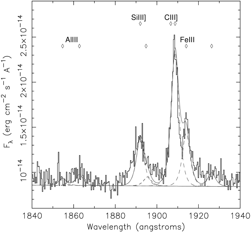
Figure 6: Model for the 1900Å feature in Ark 564. Diamonds mark the rest wavelength positions of the emission lines. The very narrow lines allow the pumped Fe III$\lambda 1914$ feature to be unambiguously detected.

Figure 7: Various parameters as a function of the asymmetry parameter. Stars mark IRAS 13224$-$3809 and 1H 0707$-$495, and open circles mark objects with significant C IV associated absorption lines; their profiles and equivalent widths are uncertain because of assumptions made to reconstruct the profiles (see Section 3). Equivalent widths (EW) are given in units of Angstroms. $\alpha_{ox}$ ($F(E)\propto E^{\alpha_{ox}}$) is defined between 2500Å and 2 keV in the rest frame. $\alpha_{u}$ ($F(\lambda)\propto\lambda^{\alpha_{u}}$) is obtained as a byproduct of the UV Fe II subtraction, and is defined between approximately 2200 Å and 3050 Å. Top and second panels: the dashed line shows the predicted relationship between equivalent width and kurtosis and asymmetry parameter for a two-component line comprised of a wind and symmetric component (see text).

Figure 8: Measured equivalent widths as a function of $\lambda L_{\lambda}$ at 1450Å. Symbols have the same meaning as in Fig. 7. Dashed lines are the Baldwin effect regressions computed by Dietrich et al. 2002. Note that for the purpose of this plot, luminosities were computed using the cosmological parameters assumed by Dietrich et al. (2002).

Figure 9: Intermediate-ionization line equivalent widths as a function of the ratio of C III] to C IV and the ratio of Si III] to C III]. Symbols have the same meaning as in Fig. 7.

Figure 10: Velocity widths of C II] and Mg II as a function of H$\beta$ velocity width. Stars denote IRAS 13224$-$3809 and 1H 0707$-$495.

Table 1: Observing log

Target	Date	Spectrometer	Observed Wavelength	Resolution	Aperture	Exposure
			(Å)	(Å)	(arc seconds)	(seconds)
IRAS 13224$-$3809	1999-06-05	HST STIS G230L	1568–3184	3.2	$0.5\times 0.24$	4457
	1999-06-05	HST STIS G140L	1140–1730	1.2	$0.5\times 0.24$	8188
	1999-06-20	CTIO 4m	3870–7570	3.0	$1\times 4$	3600
1H 0707$-$495	1999-02-16	HST STIS G230L	1568–3184	3.2	$0.5\times 0.24$	2196
	1999-02-16	HST STIS G140L	1140–1730	1.2	$0.5\times 0.24$	5376
	1998-01-04	CTIO 1.5m	3500–6940	5.5	$1.8\times 7$	1800

Table 2: Emission Line Measurements

Emission line	IRAS 13224$-$3809			1H 0707$-$495			Average EWs (Å)
	Flux	Equivalent Width	Width	Flux	Equivalent Width	Width	Francis	Zheng	Brotherton
	($\times 10^{-14}\,\rm erg\,cm^{-2}\,s^{-1}$)	(Å)	($\rm km\,s^{-1}$)	($\times 10^{-14}\,\rm erg\,cm^{-2}\,s^{-1}$)	(Å)	($\rm km\,s^{-1}$)
Ly$\alpha$+N V feature	59.4	42		166	45.9		52		87
Ly$\alpha$ (broad)	19.9	14.0		65.3	17.7			85
Ly$\alpha$ (narrow)	8.3	6.0	1160	20.2	5.6	1135
N V (broad)	27.9	20.5		57.8	16.4			10
1400 Å feature	11.4	9.6		28.3	9.9		10	7.3	8
Si IV (broad)	$5.5<7.2$	$4.6<6.1$		$10.1<15.9$	$3.5<5.6$
Si IV (narrow)	$0.75<3.7$	$0.63<3.2$		$4.5<10.6$	$1.6<3.7$
O IV (broad)	$3.7<10.2$	$3.1<8.6$		$9.4<22.4$	$3.3<7.9$
O IV (narrow)	$1.3<3.4$	$1.1<2.9$		$2.3<7.6$	$0.8<2.7$
C IV (broad)	14.6	12.8		31.3	11.6		37	59	33
He II (broad)	3.1	2.8		8.3	3.2		12	3.9	7.0
1900 Å feature	17.0	19.0		42.5	18.3		22		17
Al III	3.5	3.7	1835	8.6	3.7	3500		3.5
Si III]	6.5	7.2	1835	15.7	6.8	3500		3.5
C III]	4.7	5.3	1835	11.9	5.2	3500		17.0
Mg II	6.7	17.3	866	11.6	10.7	1050	50	64	34
C II$\lambda 1335$	3.5	2.9	1700	8.2	2.7	2100
C II$\lambda 2327$	1.5	2.7
N III$\lambda 1750$	1.0	1.2		4.4	2.0

Table 3: Correlation Matrix

	C IV Properties			High-ionization Line Properties					Intermediate-ionization Line Properties
Property	C IV EW	Asymmetry	Kurtosis	N V EW	N V/C IV	He II EW	He II/C IV	1400Å  EW	C III] EW	C III]/C IV	C III] FWHM
C IV EW	$\cdots$	$-5.2\times 10^{-3}$	0.10	$\cdots$	$-$0.40	$1.4\times 10^{-3}$	$\cdots$	$\cdots$	2.1	$\cdots$	$-$4.7
Asymmetry	$-5.2\times 10^{-3}$	$\cdots$	$-2.8\times 10^{-5}$	$\cdots$	0.16	$-$0.023	$\cdots$	$\cdots$	$-$1.7	$\cdots$	5.2
Kurtosis	0.10	$-2.8\times 10^{-5}$	$\cdots$	$\cdots$	$-$0.24	0.057	$\cdots$	$\cdots$	2.8	$\cdots$	$-$3.4
N V EW	$\cdots$	$\cdots$	$\cdots$	$\cdots$	$\cdots$	$\cdots$	$\cdots$	$\cdots$	$\cdots$	$\cdots$	$\cdots$
N V/C IV	$-$0.40	0.16	$-$0.24	$\cdots$	$\cdots$	$-$0.51	$\cdots$	$\cdots$	$-$0.069	2.2	$\cdots$
He II EW	$1.4\times 10^{-3}$	$-$0.023	0.057	$\cdots$	$-$0.51	$\cdots$	$\cdots$	3.9	0.16	$\cdots$	$\cdots$
He II/C IV	$\cdots$	$\cdots$	$\cdots$	$\cdots$	$\cdots$	$\cdots$	$\cdots$	$\cdots$	$\cdots$	2.0	$\cdots$
1400Å  EW	$\cdots$	$\cdots$	$\cdots$	$\cdots$	$\cdots$	3.9	$\cdots$	$\cdots$	1.8	$\cdots$	$\cdots$
C III] EW	2.1	$-$1.7	2.8	$\cdots$	$-$0.069	0.16	$\cdots$	1.8	$\cdots$	$\cdots$	$\cdots$
C III]/C IV	$\cdots$	$\cdots$	$\cdots$	$\cdots$	2.2	$\cdots$	2.0	$\cdots$	$\cdots$	$\cdots$	$\cdots$
C III] FWHM	$-$4.7	5.2	$-$3.4	$\cdots$	$\cdots$	$\cdots$	$\cdots$	$\cdots$	$\cdots$	$\cdots$	$\cdots$
Al III EW	$\cdots$	$\cdots$	$\cdots$	$\cdots$	$\cdots$	$\cdots$	$\cdots$	$\cdots$	$\cdots$	$\cdots$	$\cdots$
Al III/C III]	$-$1.4	0.078	$-$0.022	$\cdots$	$8.0\times 10^{-3}$	$-$0.26	$\cdots$	$\cdots$	$-$1.3	$\cdots$	$\cdots$
Si III] EW	$\cdots$	$\cdots$	$\cdots$	$\cdots$	$\cdots$	$\cdots$	$\cdots$	2.3	$\cdots$	$\cdots$	$\cdots$
Si III]/C III]	$\cdots$	0.86	$-$0.22	$\cdots$	0.30	$\cdots$	$\cdots$	$\cdots$	$\cdots$	1.7	$\cdots$
Mg II EW	$\cdots$	$\cdots$	$\cdots$	$\cdots$	$\cdots$	$\cdots$	$\cdots$	2.5	1.1	$\cdots$	$\cdots$
Mg II FWHM	$\cdots$	$\cdots$	$\cdots$	$\cdots$	$\cdots$	$\cdots$	$-$0.45	$\cdots$	$\cdots$	$\cdots$	$\cdots$
H$\beta$ FWHM	$\cdots$	$\cdots$	$\cdots$	$\cdots$	$\cdots$	$\cdots$	$-$4.2	$\cdots$	$\cdots$	$-$0.29	$\cdots$
$\alpha_{ox}$	0.028	$-$0.50	0.48	$\cdots$	$\cdots$	0.043	4.7	$\cdots$	$\cdots$	$\cdots$	$-$0.87
$\alpha_{u}$	1.9	$-$2.7	5.5	2.5	$-$4.4	0.45	$\cdots$	0.30	3.1	$\cdots$	$\cdots$
$L_{2500}$	$\cdots$	$\cdots$	$\cdots$	$\cdots$	$\cdots$	$\cdots$	$\cdots$	$\cdots$	$-$4.4	$\cdots$	$\cdots$

Note. — Percentage probability that the observed correlation is accidental are listed when the value is less than 6 (i.e., greater than 94% confidence that correlation is real).

Table 3: Correlation Matrix (cont.)

	Intermediate-ionization Line Properties (cont.)				Low-ionization Line Properties			Continuum Properties
Property	Al III EW	Al III/C III]	Si III] EW	Si III]/C III]	Mg II EW	Mg II FWHM	H$\beta$ FWHM	$\alpha_{ox}$	$\alpha_{u}$	$L_{2500}$
C IV EW	$\cdots$	$-$1.4	$\cdots$	$\cdots$	$\cdots$	$\cdots$	$\cdots$	0.028	1.9	$\cdots$
Asymmetry	$\cdots$	0.078	$\cdots$	0.86	$\cdots$	$\cdots$	$\cdots$	$-$0.50	$-$2.7	$\cdots$
Kurtosis	$\cdots$	$-$0.022	$\cdots$	$-$0.22	$\cdots$	$\cdots$	$\cdots$	0.48	5.5	$\cdots$
N V EW	$\cdots$	$\cdots$	$\cdots$	$\cdots$	$\cdots$	$\cdots$	$\cdots$	$\cdots$	2.5	$\cdots$
N V/C IV	$\cdots$	$8.0\times 10^{-3}$	$\cdots$	0.30	$\cdots$	$\cdots$	$\cdots$	$\cdots$	$-$4.4	$\cdots$
He II EW	$\cdots$	$-$0.26	$\cdots$	$\cdots$	$\cdots$	$\cdots$	$\cdots$	0.043	0.45	$\cdots$
He II/C IV	$\cdots$	$\cdots$	$\cdots$	$\cdots$	$\cdots$	$-$0.45	$-$4.2	4.7	$\cdots$	$\cdots$
1400Å  EW	$\cdots$	$\cdots$	2.3	$\cdots$	2.5	$\cdots$	$\cdots$	$\cdots$	0.30	$\cdots$
C III] EW	$\cdots$	$-$1.3	$\cdots$	$\cdots$	1.1	$\cdots$	$\cdots$	$\cdots$	3.1	$\cdots$
C III]/C IV	$\cdots$	$\cdots$	$\cdots$	1.7	$\cdots$	$\cdots$	$-$0.29	$\cdots$	$\cdots$	$-$4.4
C III] FWHM	$\cdots$	$\cdots$	$\cdots$	$\cdots$	$\cdots$	$\cdots$	$\cdots$	$-$0.87	$\cdots$	$\cdots$
Al III EW	$\cdots$	$\cdots$	$1.3\times 10^{-4}$	0.79	2.4	$\cdots$	$\cdots$	$\cdots$	$\cdots$	$\cdots$
Al III/C III]	$\cdots$	$\cdots$	$\cdots$	0.010	$\cdots$	$\cdots$	$\cdots$	$-$4.3	$\cdots$	$\cdots$
Si III] EW	$1.3\times 10^{-4}$	$\cdots$	$\cdots$	2.4	0.28	$\cdots$	$\cdots$	$\cdots$	$\cdots$	$\cdots$
Si III]/C III]	0.79	0.010	2.4	$\cdots$	$\cdots$	$\cdots$	$\cdots$	$\cdots$	$\cdots$	$\cdots$
Mg II EW	2.4	$\cdots$	0.28	$\cdots$	$\cdots$	$\cdots$	$\cdots$	$\cdots$	$\cdots$	$\cdots$
Mg II FWHM	$\cdots$	$\cdots$	$\cdots$	$\cdots$	$\cdots$	$\cdots$	$\cdots$	$\cdots$	$\cdots$	0.40
H$\beta$ FWHM	$\cdots$	$\cdots$	$\cdots$	$\cdots$	$\cdots$	$\cdots$	$\cdots$	$\cdots$	$\cdots$	5.9
$\alpha_{ox}$	$\cdots$	$-$4.3	$\cdots$	$\cdots$	$\cdots$	$\cdots$	$\cdots$	$\cdots$	$\cdots$	$\cdots$
$\alpha_{u}$	$\cdots$	$\cdots$	$\cdots$	$\cdots$	$\cdots$	$\cdots$	$\cdots$	$\cdots$	$\cdots$	$\cdots$
$L_{2500}$	$\cdots$	$\cdots$	$\cdots$	$\cdots$	$\cdots$	0.40	5.9	$\cdots$	$\cdots$	$\cdots$

Note. — Percentage probability that the observed correlation is accidental are listed when the value is less than 6 (i.e., greater than 94% confidence that correlation is real).

Table 4: Principal Components Analysis Results

Parameter	Eigenvector 1	Eigenvector 2	Eigenvector 3
C IV EW	0.32	0.02	0.01
Asymmetry	$-$0.32	0.06	0.01
Kurtosis	0.32	$-$0.08	$-$0.09
N V EW	0.02	0.21	0.27
N V/C IV	$-$0.29	0.05	$-$0.24
He II EW	0.33	0.07	$-$0.05
He II/C IV	0.06	0.15	$-$0.42
1400Å  EW	0.17	0.26	0.18
C III] EW	0.26	0.16	0.14
C III]/C IV	$-$0.11	0.27	$-$0.33
C III] FWHM	$-$0.21	0.06	0.31
Al III EW	$-$0.06	0.40	0.16
Al III/C III]	$-$0.30	0.16	$-$0.02
Si III] EW	$-$0.01	0.42	0.15
Si III]/C III]	$-$0.23	0.32	$-$0.02
Mg II EW	0.12	0.26	0.27
Mg II] FWHM	$-$0.09	$-$0.23	0.30
H$\beta$] FWHM	0.06	$-$0.23	0.34
$\alpha_{ox}$	0.28	$-$0.02	$-$0.20
$\alpha_{u}$	0.24	0.19	0.12
$L_{2500}$	$-$0.17	$-$0.27	0.20
Cumulative Fraction of Variance	0.38	0.60	0.78

References

- Baldwin (1977) Baldwin, J. A., 1977, ApJ, 214, 679
- Baldwin (1997) Baldwin, J. A., 1997, Proc. “Emission Lines in Active Galaxies: New Methods and Techniques”, eds. B. M. Peterson, F.-Z. Cheng, & A. S. Wilson (ASP: San Francisco) p. 80
- Baldwin et al. (1996) Baldwin, J. A., Ferland, G. J., Korista, K. T., Carswell, R. F., Hamann, F., Phillips, M. M., Verner, D., Wilkes, B. J., & Williams, R. E., 1996, ApJ, 461, 664
- Ballantyne, Iwasawa & Fabian (2001) Ballantyne, D. R., Iwasawa, K., & Fabian, A. C., 2001, MNRAS, 323, 506
- Blades et al. (1988) Blades, J. C., Wheatley, J. M., Panagia, N., Grewing, M., Pettini, M., & Wamsteker, W., 1988, ApJ, 334, 309
- Boller et al. (1993) Boller, Th., Trümper, J., Molendi, S., Fink, H., Schaeidt, S., Caulet, A., & Dennefeld, M., 1993, A&A, 279, 53
- Boller, Brandt & Fink (1996) Boller, Th., Brandt, W. N., & Fink, H., 1996, A&A, 305, 53
- Boller et al. (1997) Boller, Th., Brandt, W. N., Fabian, A. C., & Fink, H. H., 1997, MNRAS, 289, 393
- Boller, Brandt & Fink (1996) Boller, T., Brandt, W. N., & Fink, H., 1996, A&A, 305, 53
- Boller et al. (2002) Boller, Th., Fabian, A. C., Sunyaev, R., Trümper, J., Vaughan, S., Ballantyne, D. R., Brandt, W. N., Keil, R., & Iwasawa, K., 2002, MNRAS, 329, L1
- Boller et al. (2003) Boller, Th., Tanaka, Y., Fabian, A. C., Brandt, W. N., Gallo, L., Anabuki, N., Haba, Y., & Vaughan, S., 2003, MNRAS, in press
- Boroson (2002) Boroson, T. A., 2002, ApJ, 565, 78
- Boroson & Green (1992) Boroson, T. A., & Green, R. F., 1992, ApJS, 80, 109
- Boroson & Meyers (1992) Boroson, T. A., & Meyers, K. A., 1992, ApJ, 397, 442
- Brandt, Mathur & Elvis (1997) Brandt, W. N., Mathur, S., & Elvis, M., 1997, MNRAS, 285, L25
- Brandt, Laor & Wills (2000) Brandt, W. N., Laor, A., Wills, B. J., 2000, ApJ, 528, 637
- Brotherton et al. (2001) Brotherton, M. S., Tran, H. D., Becker, R. H., Gregg, M. D., Laurent-Muehleisen, S. A., & White, R. L., 2001, ApJ, 546, 775
- Cardelli, Clayton & Mathis (1989) Cardelli, J. A., Clayton, G. C., & Mathis, J. S., 1992, ApJ, 345, 245
- Casebeer and Leighly (2004) Casebeer, D., & Leighly, K. M., 2004, to be submitted to ApJ
- Collin-Souffrin et al. (1988) Collin-Souffrin, S., Dyson, J. E., McDowell, J. C., & Perry, J. J., 1988, MNRAS, 232, 539
- Comastri et al. (1998) Comastri A., et al. 1998, A&A, 333, 31
- Corbin & Boroson (1996) Corbin, M. R., & Boroson, T. A., 1996, ApJS, 107, 69
- Crenshaw et al. (2002) Crenshaw, D. M., et al., 2002, ApJ, 566, 187
- Crenshaw, Kraemer, & Gabel (2003) Crenshaw, D. M., Kraemer, S. B., & Gabel, J. R., 2003, AJ, 126, 1690
- Dewangen et al. (2002) Dewangen, G. C., Boller, Th., Singh, K. P., & Leighly, K. M., 2002, A&A, 390, 65
- Dietrich et al. (2002) Dietrich, M., Hamann, F., Shields, J. C., Constantin, A., Vestergaard, M., Chaffee, F., Foltz, C. B., & Junkkarinen, V. T., 2002, ApJ, 581, 912
- Ferland (2001) Ferland, G. J., 2001, “Hazy, a Brief Introduction to Cloudy 96.00”
- Flower and Nussbaumer (1975) Flower, D. R., & Nussbaumer, H., 1982, A&A, 45, 145
- Francis et al. (1991) Francis, P. J., Hewett, P. C., Foltz, C. B., Chaffee, F. H., Weymann, R. J., & Morris, S. L., 1991, ApJ, 373, 465
- Goodrich (1989) Goodrich, R. W. 1989, ApJ, 342, 224
- Graham, Clowes & Campusano (1996) Graham, M. J., Clowes, R. G., & Campusano, L. E., 1996, MNRAS, 279, 1349
- Grupe et al. (1998) Grupe, D., Beuermann, K., Thomas, H.-C., Mannheim, K., & Fink, H. H., 1998, A&A, 330, 25
- Grupe & Leighly (2002) Grupe, D., & Leighly, K. M. 2002, Proc. “Workshop on X-ray Spectroscopy of AGN with Chandra and XMM–Newton”, eds. Th. Boller, S. Komossa, S. Kahn, H. Kunieda, & L. Gallo (MPE: Garching) p. 259
- Grupe et al. (2000) Grupe, D., Leighly, K. M., Thomas, H.-C., & Laurent-Muehleisen, S. A., 2000, A&A, 356, 11
- Grupe et al. (2001) Grupe, D., Thomas, H.-C., & Leighly, K. M., 2001, A&A, 369, 450
- Harper et al. (1999) Harper, G. M., Jordan, C., Judge, P. G., Robinson, R. D., Carpenter, K. G., & Brage, T., 1999, MNRAS, 303, 41
- Hartig & Baldwin (1986) Hartig, G. F., & Baldwin, J. A., 1986, ApJ, 302, 64