A Strong, Broad Absorption Feature in the X-ray Spectrum of the Nearby Neutron Star RX J1605.3+3249

Abstract

We present X-ray spectra taken with XMM-Newton of RX J1605.3+3249, the third brightest in the class of nearby, thermally emitting neutron stars. In contrast to what is the case for the brightest object, RX J1856.5$-$3754, we find that the spectrum of RX J1605.3+3249 cannot be described well by a pure black body, but shows a broad absorption feature at 27 Å (0.45 keV). With this, it joins the handful of isolated neutron stars for which spectral features arising from the surface have been detected. We discuss possible mechanisms that might lead to the features, as well as the overall optical to X-ray spectral energy distribution, and compare the spectrum with what is observed for the other nearby, thermally emitting neutron stars. We conclude that we may be observing absorption due to the proton cyclotron line, as was suggested for the other sources, but weakened due to the strong-field quantum electrodynamics effect of vacuum resonance mode conversion.

1 Introduction

The nearby, thermally emitting, radio-quiet neutron stars offer the best possibilities for measuring spectra directly from a neutron-star surface, uncontaminated by emission due to accretion and/or magnetospheric processes. Since the serendipitous discovery of the first of these in 1996 by Walter et al., six (possibly seven) more have been uncovered in the ROSAT All-Sky Survey (see reviews by Treves et al. 2000; Haberl 2004). For four sources, optical counterparts have been identified (Walter & Matthews 1997; Motch & Haberl 1998; Kulkarni & van Kerkwijk 1998; Kaplan et al. 2002a, 2003a). The high X-ray to optical flux ratios leave no model but an isolated neutron star.

At present, it is not clear what is the source of the thermal emission. The possibilities considered range from slow accretion from the interstellar medium to release of residual heat, to decay of strong magnetic fields. Most important for the present purposes, however, is that all six sources appear to have X-ray spectra that, as far as one can tell from current observations, are entirely thermal, thus offering the hope that it will be possible to do a ‘standard’ model-atmosphere analysis, and infer precise values of the temperature, surface gravity, gravitational redshift and magnetic field strength.

Given their interest, the nearby, thermally emitting neutron stars have been among the prime targets for spectroscopy with the Chandra X-ray Observatory and XMM-Newton. First XMM results on the second-brightest in the class, RX J0720.4$-$3125 (Paerels et al. 2001), were somewhat disappointing, as no lines were found. The first Chandra spectra, of the brightest thermally emitting neutron star, RX J1856.5$-$3754, also revealed no lines (Burwitz et al. 2001). Indeed, even a much longer (500 ks) integration failed to show evidence for any features, showing instead a spectrum remarkably well described by a black body affected only by interstellar extinction (Drake et al. 2002; Braje & Romani 2002; Burwitz et al. 2003). Similarly, Chandra data on the Vela pulsar (Pavlov et al. 2001) and PSR B0656+14 (Marshall & Schulz 2002), both of which have strong thermal components in their X-ray spectra, failed to show any features.

The only exceptions came recently. First, Sanwal et al. (2002) discovered two absorption features in Chandra observations of 1E 1207.4$-$5209, the pulsating central source in the supernova remnant PKS 1209$-$51/52. Variability in these features as a function of pulse phase was seen in XMM observations by Mereghetti et al. (2002), and confirmed by Bignami et al. (2003), who also reported a third and possibly even a fourth feature, all harmonically spaced. The nature of the absorption features is not yet clear, with suggestions ranging from cyclotron lines to transitions of Helium or mid-Z atoms in a strong magnetic field (Sanwal et al. 2002; Hailey & Mori 2002). Second, Haberl et al. (2003a) discovered a broad absorption feature in XMM spectra of RX J1308.6+2127, a nearby, thermally emitting neutron star. As before, it is not clear what causes the feature; Haberl et al. speculate it might be due to proton cyclotron absorption. Third, while we were revising of our manuscript, a preprint by Haberl et al. (2003b) showed that another nearby neutron star, RX J0720.4$-$3125 had a broad, but weaker absorption feature as well, contrary to earlier claims (Paerels et al. 2001; Pavlov et al. 2001; Kaplan et al. 2003b).

Here, we present the discovery of a broad absorption feature in a third nearby, thermally emitting neutron star, RX J1605.3+3249. We describe our observations and reduction in § 2. In § 3, we analyze and characterize the spectrum, and in § 4, we derive limits to any periodic variations. We discuss implications for our understanding of RX J1605.3+3249, as well as the nearby, thermally emitting neutron stars in general, in § 5.

Table 1: Summary of X-ray Observations

ObsID	Instrument	Mode	Start Time	Exposure		Count Rate
				Raw	Filtered
			(UT)	(ks)	(ks)	(${\rm s}^{-1}$)
2791	ACIS-I	Standard	2002 Jan 07.17	20.4	20.4	0.153
0073140301	EPIC-PN	Timing	2002 Jan 10.04	26.0	14.3	3.118(16)
	RGS1/RGS2	Standard		33.6	20.9/19.4	0.139(3)/0.130(3)
0073140201	EPIC-PN	Timing	2002 Jan 15.99	26.4	24.2	3.083(12)
	RGS1/RGS2	Standard		30.4	27.8/27.0	0.138(3)/0.127(3)
0073140501	EPIC-PN	Timing	2002 Jan 19.97	29.8	18.4	3.069(14)
	RGS1/RGS2	Standard		33.9	22.2/21.5	0.141(3)/0.133(3)
0157360401	EPIC-PN	Large-window	2003 Jan 17.91	33.2	25.7	2.385(10)
	RGS1/RGS2	Standard		41.7	31.3/31.2	0.144(2)/0.133(2)
0157360601	EPIC-PN	Large-window	2003 Feb 26.80	16.8	8.8	1.477(13)
	RGS1/RGS2	Standard		32.2	10.1/09.5	0.148(5)/0.147(6)

2 X-ray observations

We observed RX J1605.3+3249 with XMM three times, on 9, 15, and 19 January 2002, for a total of approximately 100 ks. In addition, we analysed XMM data taken for calibration purposes on 18 January and 27 February 2003, and data taken with Chandra on 7 January 2002. A summary is given in Table 1.

2.1 XMM

XMM consists of three X-ray telescopes (Jansen et al. 2001). For two of these, half the light is deflected to Reflection Grating Spectrometers (RGS; den Herder et al. 2001), while the other half is fed to European Photon Imaging Cameras with MOS detectors (EPIC-MOS; Turner et al. 2001). A third camera, with PN detectors (EPIC-PN; Strüder et al. 2001) receives all the light of the third telescope.

2.1.1 EPIC-MOS imaging

As RX J1605.3+3249 is bright, photon pile-up, where multiple photons arrive in one integration time, is a concern. We had hoped to use the EPIC MOS detectors in a mode in which the central chip is read out fast, but this had not yet been commissioned at the time of the observations. We decided to use full-frame mode instead (2.6-s frame time), sacrificing spectral and timing information for field of view, hoping to increase the number of background sources and hence improve the absolute astrometry. This objective became moot with the measurement of an accurate Chandra position: $\alpha_{\rm J2000}=16^{\rm h}05^{\rm m}18\fs 50\pm 0\fs 06$, $\delta_{\rm J2000}=+32^{\circ}49^{\prime}17\farcs 4\pm 0\farcs 7$ (Kaplan et al. 2003a). The observations were taken through the thin filter, in order to maximize the soft response. The same setup happened to be used for the calibration observations.

We reprocessed the three observations using the standard task emchain in the XMM Science Analysis System (XMM-SAS), version 5.4.1. We determined the positions of RX J1605.3+3249 in both cameras and all observations and found these to be fully consistent with the Chandra position mentioned above (within 3″ before aspect correction). We used the MOS positions in the RGS and PN-timing reduction to define the source position in the local, satellite frame.

Figure 1: Flux-calibrated RGS spectrum of RX J1605.3+3249, binned to 0.175 Å. At this binning, all points are uncorrelated, independent flux measurements. The total integration time is 110 ks. Overdrawn are two fits: slightly extincted black body curves with one (lower dotted line) and two Gaussian (lower continuous curve) absorption features. The upper curves reflect the corresponding continua ($n_{\rm c}(\lambda)$ in Eq. 1).

2.1.2 RGS spectroscopy

For the RGS observations, we used the standard ‘High Event Rate with SES’ spectroscopy mode for read-out. We reprocessed the data using the XMM-SAS routine, rgsproc. We first made event files and determined times of low background from the count rate on CCD 9 (which is closest to the optical axis), rejecting all times that the rate was above 0.5$\rm\,s^{-1}$. The final exposure times and net count rates are listed in Table 1. Source and background counts were extracted using the standard spatial and energy filters; for the source position, which defines the spatial extraction regions as well as the wavelength zero point, we used the position inferred from the corresponding EPIC-MOS camera and exposure. As the source showed no sign of variability, we combined all spectra into one flux-calibrated average using the task rgsfluxer. The result, binned to 0.175 Å, is shown in Fig. 1.

2.1.3 EPIC-PN spectroscopy

Timing mode.

For the 2002 PN observations, we used the timing mode, in order to avoid pile-up and to allow a search for variability at as large a range of periods as possible. In this mode, the central CCD is read out continuously, and hence the gain in time resolution comes at the cost of loss of positional information along the detector columns and increased background. The observations were taken through the thin filter in order to maximize the response at low energies.

We reprocessed the data using the XMM-SAS task epchain, using the EPIC-MOS1 position as a reference for timing purposes. We extracted source spectra in a region of 17 pixels centered on the peak of the (one-dimensional) point-spread function ($31\leq{\rm rawx}\leq 47$). For the background, we used a region of the same size away from the source ($6\leq{\rm rawx}\leq 22$). For both, we excluded times of high background due to proton flares (rejecting all 52-s intervals in which the 0.3–1 keV background count rate exceeded 0.25 s^-1).

Figure 2: Count spectra for the timing mode EPIC-PN data taken on 15 January 2002. The top two curves are for the single-pixel events for the source (bold) and background region, while the bottom two curves are for the double-pixel events. The strong peaks at low energies are instrumental, and have different strength for the source and background regions. If not taken into account, the peak in the double-pixel events will lead to artificial features in the background-corrected spectrum.

Looking in detail at the count spectrum for the timing data (see Fig. 2), we found a peculiar excess of counts with energies just above 0.2 keV for single-pixel events, and energies just above 0.4 keV for double-pixel events. Inspecting the event file, it seems that these are due to flickering, ‘hot’ pixels, which lead to bursts of events over short periods of time. Many of these follow each other sufficiently rapidly that in the data stream they appear as neighbouring events and thus are identified by the pipeline as double-pixel events. These hot pixels pose a problem, as their number is not the same in the source and background regions. Hence, if not taken into account, one will obtain instrumental emission or absorption features around 0.2 and 0.4 keV. The latter is exactly in the range where we find absorption in the RGS spectra (§ 3.1).

Because of the above, for our spectroscopic analysis we had at first decided to use only the single-pixel events, generating response matrices for this selection using the appropriate SAS tasks. However, we learned (F. Haberl, 2003, personal comm.) that for single-pixel events in timing mode the response is not very well understood, and that only the combination of singles and doubles at energies above 0.5 keV gives reliable, reproduceable results. Indeed, the SAS task generates a response valid for this combination (R. Saxton, 2003, personal comm.; oddly, the results were consistent nevertheless – see § 3.2). It seems possible to circumvent these problems by careful excision of the burst of noise events (Burwitz et al. 2004), but we decided to forego this excercise, since for the large-window data the response at low energies is fairly secure.

Large window mode.

For the calibration data taken in large-window mode, we again ran the standard task epchain, and rejected time intervals with strong background flaring using the standard good-time intervals (for which the all-chip 7–15 keV count rate is below 10 s^-1). We selected source events within an aperture of $64\farcs 5$ radius, and background events from an annulus with radii between 80 and $100\arcsec$; this means that our background is not all taken from the same chip, but given the very large source count rate, the effect of this is minimal. Indeed, the count rate of the source is sufficiently high, $2.4\rm\,s^{-1}$, that despite the 48-ms frame time offered by large-window mode there will be some pile up: in some integrations two photons will hit the detector so closely to each other that the resulting charge distribution will be identified as a single event (with anomalously high energy). Our source is very soft, essentially following a Wien tail at higher energies; as a result, even a small fraction of piled up events can give the false impression of a hard tail. Comparing the spectra of single and double-pixel events, we find this to be the case. Therefore, we decided to use single-pixel events only. We note that even with those, we see some evidence for pile up at the higher energies. As it is a small effect, however, we felt it not worthwhile to try to ameliorate this by cutting out the core of the point-spread function, in particular as the uncertainty in how the point-spread function varies as a function of energy may well be larger than any residual effects due to pile-up. Instead, we simply conclude that while the large-window mode data should give a more secure view of what happens at low energies, the timing-mode data are to be trusted better at high energies.

2.2 Chandra

For the Chandra data, we first reprocessed the level-1 event file into a level-2 event file, following standard procedures, while keeping the events that had been flagged as possible afterglow. We also took advantage of an updated response file and corrected for the charge transfer inefficiency of the ACIS S3 detector, on which the source was located. We used the CIAO tool psextract to extract source and background spectra – from a circular region centered on RX J1605.3+3249 with a radius of 4 pixels, and an annulus from radii of 20 pixels to 45 pixels, respectively – as well as to create the response files. To account for the slight degradation with time of the ACIS detectors, we applied a correction appropriate for our observing date. Due to the 3.2-s frame time of the ACIS-I observations, RX J1605.3+3249 suffers from significant pileup (the count-rate was $\approx 0.15\mbox{ s}^{-1}$). We therefore used the Sherpa pileup model (Davis, 2001) when analyzing the data. We note that the Sherpa pile-up model can give erroneous results if one tries to determine which spectral shape fits the data best. It should suffice, however, for our purpose of cross-checking the XMM results.

3 The spectrum

The flux-calibrated RGS spectrum (Fig. 1) is clearly inconsistent with a smooth function like an absorbed black body, unlike what is seen for RX J1856.5$-$3754, the brightest thermally emitting neutron star (see § 1). In order to quantify the departures, we tried fitting black bodies with simple absorption features, and compare the results between the different instruments.

Before describing the results, we should stress that there are still energy-dependent inconsistencies between the calibration of EPIC-pn and RGS at the $\lesssim\!20$% level (M. Sako, J.-W. den Herder, 2003, personal communications; Kirsch 2003; Fig. 4 below), especially below $\sim\!0.5\,$keV, and it is not known which is correct.

3.1 Fitting the RGS Data

We start with the RGS data, as these have the best resolution. We rebin them to 0.175 Å, as shown in Fig. 1. As expected from the figure, a black body gives an unsatisfactory fit, with a reduced $\chi^{2}$ of 2.6 (for 170 degrees of freedom), and with a best-fit column density $N_{H}$ of zero (see Table 2).

As a first-order parametrisation of the deviations from a black body, we include Gaussian absorption features, as follows,

$$n(\lambda)=n_{\rm c}(\lambda)\prod_{i}\left[1-r_{i}\exp\left(-4\log 2\frac{(\lambda-\lambda_{i})^{2}}{{\rm FWHM}_{i}^{2}}\right)\right]$$ (1)

where $n(\lambda)$ is the photon rate per unit wavelength at wavelength $\lambda$, $n_{\rm c}(\lambda)$ the continuum photon rate (in our case the extincted black body), and $r_{i}$, $\lambda_{i}$ and FWHM_i are the fractional depth, central wavelength, and full width at half maximum of the Gaussian feature.

We find that the inclusion of a single Gaussian improves the quality of the fit dramatically, changing the reduced $\chi^{2}$ from 2.6 to 0.9, i.e., a good fit (see Fig. 1; Table 2). The Gaussian is centered at 27.3 Å (0.45 keV), and has a FWHM of 13 Å (0.2 keV). Since this Gaussian is so broad, covering a significant fraction of the spectrum, its amplitude is highly covariant with the other fit parameters that determine the overall shape of the spectrum ($N_{\rm H}$, $kT$, and $R_{\infty}/d$); all these, therefore, have rather large uncertainties.

In Fig. 1, it looks like there is also a narrower absorption feature, at $\sim\!22\,$Å. We included a second Gaussian in the fit and found a central wavelength of 21.5 Å (0.58 keV), and a FWHM of 0.5 Å (0.12 keV); see Table 2. This wavelength is close to that of the resonance line of He-like Oxygen (O VII), but it would be hard to understand as interstellar absorption, given both the large equivalent width and the fact that it is resolved. It is unlikely to be an instrumental artifact, as we do not see it in RGS spectra of other thermally emitting neutron stars. Thus, it may come from the neutron-star surface. We stress, however, that the detection needs to be confirmed: while the line itself is significant at the 3.5-$\sigma$ level, the significance of the feature decreases to marginal once one takes into account properly the number of trials (of order 100) associated with looking anywhere in the spectrum for absorption features. Independent of its significance, one thing to note is how strongly the addition of even this small line affects the inferred continuum (see Fig. 1). This is due to the above-mentioned covariance between the various parameters.

Table 2: Fits to the RGS and EPIC spectra

Parameter	RGS			EPIC
	0-G	1-G	2-G	0-G	1-GE	1-G
$N_{H}$ $(\times 10^{20}{\rm cm}^{-2})$	0	2.2(11)	0.8(10)	0	0.68(10)	0.98(19)
$kT$ (eV)	105.0(11)	90(4)	95(4)	98.00(15)	94.1(5)	92.6(8)
$R_{\infty}/d$ (km/kpc)	6.66(17)	15(4)	11(2)	9.10(4)	11.0(3)	12.0(6)
$r_{1}$	$\cdots$	0.55(10)	0.42(8)	$\cdots$	0.258(16)	0.28(2)
$\lambda_{1}$ (Å)	$\cdots$	27.3(3)	25.71(15)	$\cdots$	24.75(15)	25.4(2)
${\rm FWHM}_{1}$ (Å)	$\cdots$	17(3)	13(2)	$\cdots$	6.7(5)	8.9(12)
${\rm EW}_{1}$ (Å)	$\cdots$	10	6	$\cdots$	1.8	2.7
$r_{2}$	$\cdots$	$\cdots$	0.27(7)	$\cdots$	$\cdots$	$\cdots$
$\lambda_{2}$ (Å)	$\cdots$	$\cdots$	21.52(6)	$\cdots$	$\cdots$	$\cdots$
${\rm FWHM}_{2}$ (Å)	$\cdots$	$\cdots$	0.46(16)	$\cdots$	$\cdots$	$\cdots$
${\rm EW_{2}}$ (Å)	$\cdots$	$\cdots$	0.13	$\cdots$	$\cdots$	$\cdots$
$\chi^{2}$	445	152	139	542	291	281
DOF	170	167	164	144	141	141
$\chi^{2}/$DOF	2.62	0.91	0.85	3.77	2.06	2.00

Note. — The second row in the header refers to the type of the fit: 0-G: black-body continuum only; 1-G: including one Gaussian absorption component (in wavelength units); 2-G: including two Gaussian absorption components; 1-G_E: one Gaussian in energy units. The parameters $r$, $\lambda$, FWHM, and EW are the fractional depth, central wavelength, full width at half maximum, and equivalent width of the Gaussian feature (for a Gaussian, ${\rm EW}=r\sqrt{\pi/4\log 2}\,{\rm FWHM}$). The numbers in parentheses are 1-$\sigma$ uncertainties in the last digit (determined by varying the parameter while leaving all other parameters free).

3.2 Determining the continuum

The EPIC-pn data cover a larger range in energy and hence might help to determine the shape of the overall continuum. We fit the four data sets taken through the thin filter jointly. For this purpose, we rebinned all data sets to have a similar number of counts in each bin and a bin width of $\sim\!20\,$eV, which is roughly one third of the spectral resolution. For the three timing-mode data sets we used the singles plus doubles at $>\!0.5\,$keV, and for the large-window mode data set we used singles only at $>\!0.15\,$keV. As expected from the RGS data, we find that a simple absorbed blackbody does not work: the implied column density is again $N_{\rm H}=0$, and the reduced $\chi^{2}_{\rm red}$ is an unacceptable 4.4 (Table 2). The residuals, shown in Fig. 3, deviate significantly from a smooth spectrum, with the largest deviation at energies near 0.45 keV (28 Å), just where the RGS data showed the broad absorption feature (Fig. 1). In this region, there are no known instrumental edges, etc.

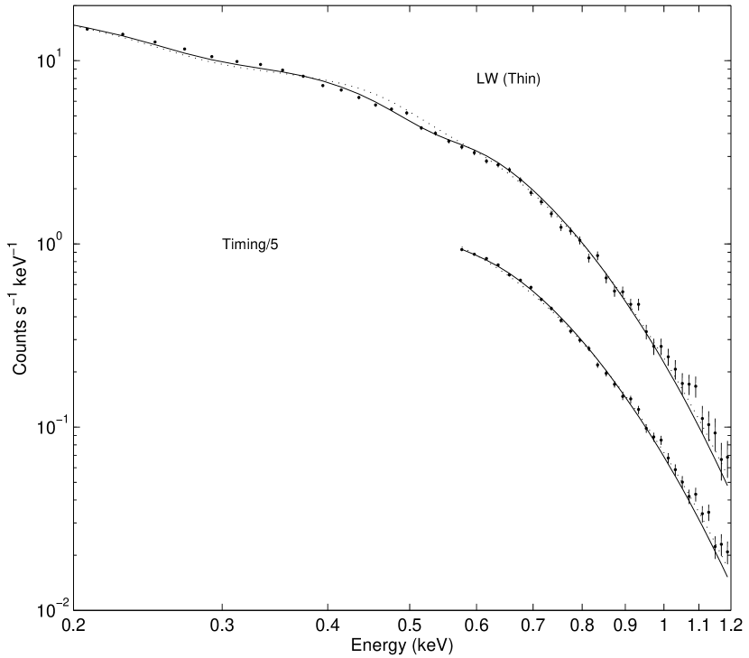
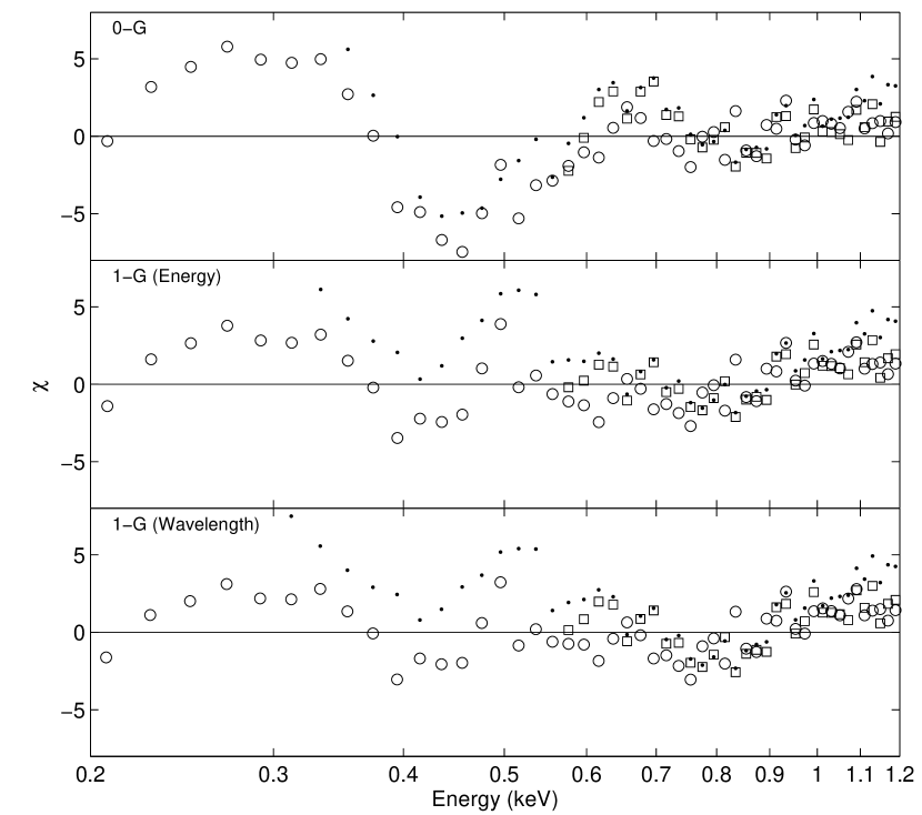
Figure 3: Fits and residuals to the XMM EPIC data taken through the thin filter. The top panel shows the observations, as well as the best fits using a single black body (dotted curve) and a black body with one Gaussian-shaped absorption feature (continuous curve). The bottom panels show the residuals for these two cases, as well as for the best fit of a black body with a single Gaussian in wavelength units. The residuals for the observations taken in large-window mode are shown by circles, those in timing mode by squares. The residuals for singles down to 0.3 keV in timing mode are shown by dots (see § 3.3).

As a first-order parametrisation, we again fit a blackbody absorbed by a Gaussian, described as in Eq. 1, but written in energy units (i.e., replacing all wavelengths in Eq. 1 with energies; the rationale is that for the EPIC CCD spectra the resolution in energy $\Delta E$ is roughly constant at low energies, while the resolution in wavelength $\Delta\lambda$ changes rapidly; for the grating spectra, the reverse holds). We find that this leads to a significant improvement, but that the fit is still unacceptable ($\chi^{2}_{\rm red}=2.0$). Indeed, although the fit to the data looks fairly good (Fig. 3), the residuals show clear systematic deviations. As the RGS fit was so much better, we wondered whether it would help to use a Gaussian in wavelength units rather than energy units (for a wide Gaussian, the shape is significantly different). Indeed, for the RGS data we find that with a Gaussian in energy units, the fit is not very good (worse than the fit using the Gaussian in wavelength units by $\Delta\chi^{2}=10$; best-fit $N_{\rm H}$ remaining at zero). For the EPIC data, the fit improves as well ($\Delta\chi^{2}=26$, no change in degrees of freedom), but the difference in the results is small (see Fig. 3; Table 2). We tried fitting more Gaussians, as well as different shapes (Lorentzians), but did not find a simple, significantly better result.

Figure 4: Unfolded spectra. The points reflect the EPIC PN data obtained in large-window mode, and the dashed curve is the best fit to them by an absorbed black body with a single Gaussian absorption feature (in wavelength units; Table 2). (Note that the uncertainties for the unfolded EPIC data are not reliable for the large bin sizes at long wavelengths. The quality of the fit should be judged from Fig. 3.) The continuous curves are the flux-calibrated RGS spectrum and its best fit (single Gaussian; Table 2).

What did become clear, however, is that the inferred shape of the continuum is rather sensitive to the choice of parametrisation. For instance, from Table 2, one sees that the results for $N_{H}$, $kT$, and $R/d$ differ significantly depending on whether one uses the Gaussian in energy or wavelength units. The difference between the results from RGS and EPIC, however, is larger still. Mostly, this reflects the inconsistencies in the calibration of the two instruments at low energies mentioned at the start of this section, as can be seen in Fig. 4, where we show the unfolded EPIC spectrum taken in large-window mode, with the flux-calibrated RGS spectrum overdrawn.

Less clear is whether these inconsistencies could explain the difference in strength of the absorption feature, the equivalent width for the RGS being a factor three larger than that for EPIC. In order to determine the significance, we fitted the RGS data forcing the equivalent width at the value found by EPIC (3.3 Å). We found that $\chi^{2}$ increased by 14, which is not a highly significant change. However, $N_{\rm H}$ became zero, which is not realistic. If we also fix $N_{\rm H}$ to the EPIC value ($1.3\times 10^{20}{\rm\,cm^{-2}}$), the fit does become significantly worse ($\Delta\chi^{2}=36$). We conclude that while we can be confident about the presence and the central wavelength of the absorption feature, we cannot measure its strength securely. In the absence of improvements in the calibration, observations at high resolution but covering a larger wavelength range, such as could be provided with the LETG on Chandra, are required to resolve this issue.

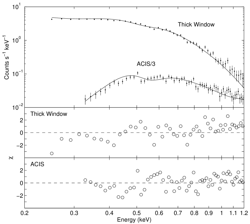
Figure 5: Comparison of the data taken with Chandra ACIS-I and XMM EPIC through the thick filter with the best fit inferred from the EPIC data taken through the thin filter (Fig. 3). Both data sets confirm that a strong absorption feature is present near 0.4 keV.

3.3 Verification

The calibration of the timing mode data, and of observations taken through the thin filter in general, is still uncertain. Therefore, we verified that the black body with a single Gaussian (in energy units) could reproduce other data sets. The first is the Chandra ACIS data. For these, there is another free parameter $\alpha$ (the pileup probability; see Davis 2001). Applying the model to the ACIS data – binned to $\sim\!15\,$eV – while fitting only for $\alpha$, we achieved a good fit (Fig. 5): $\chi^{2}=76$ for 70 degrees-of-freedom, with $\alpha=0.76\pm 0.05$, which is within the accepted range of 0.2–0.8. The uncertainties of the pileup model, especially around the instrumental features near 0.5–0.7 keV, make this fit less reliable than the EPIC data, but the fact that the two agree and that the absorption feature at 0.45 keV is easily seen gives confidence that the feature is real and that the continuum shape is close to correct.

Second, we compared the model to large-window data taken with the thick filter (binned to $\sim\!20\,$eV). Again, keeping all parameters fixed, we find $\chi^{2}=74$ for 53 degrees-of-freedom (Fig. 5); this is no worse a fit than what we found for the data taken through the thin filter.

Third, we refitted the timing data with the same model, but now selecting only singles, at energies above 0.3 keV. As mentioned in § 2.1.3, the response for this setup is not well understood. Nevertheless, the fit is no worse than that for the other data sets, and the 0.45 keV absorption feature is again obvious (see Fig. 3).

3.4 Limit on high energy flux

Unlike radio pulsars, the X-ray spectra of the thermally emitting neutron stars do not appear to require any contribution of non-thermal emission. This is the case also for RX J1605.3+3249: at energies above 2 keV, we can only set limits to the flux. Our most stringent constraints come from the EPIC-PN observations in large-window mode. In the 2–4.5 and 4.5–7.5 keV ranges, the upper limits on the count rate are 4 and $5\times 10^{-4}{\rm\,s^{-1}}$ (2$\sigma$), respectively, corresponding to limits on the flux of 3 and $9\times 10^{-15}{\rm\,erg\,s^{-1}\,cm^{-2}}$, respectively (using the standard XMM conversion factors, strictly valid only for a $N(E)\propto E^{-1.7}$ power law absorbed by $N_{\rm H}=3\times 10^{20}{\rm\,cm^{-2}}$).

Figure 6: Lightcurves for each exposure, with net count rates measured in 10-s bins. Time is measured from the start of each observation, and sections near the end that were affected by background soft proton flares have been removed. In addition, for the 2002 observations, an energy cut was used to exclude low-energy events due to hot, flickering pixels.

4 Timing Analysis

To search for periodic signals, we used the timing-mode data sets, as well as the data set taken in large-window mode through the thin filter. The data set taken through the thick filter had, relatively, too few counts to be useful. We barycentered all events using the XMM-SAS task barycen. For the timing-mode observations, we included both single-pixel and double-pixel events, but restricted the energies to ${\rm PI}>300$ and ${\rm PI}>500$, respectively, in order to exclude the noise close to the threshold mentioned above (§2.1.3; Fig. 2). We extracted source and background counts from the same regions as used for the spectra. For the large-window data, we selected both single and double-pixel events with energies above 0.2 keV, from within a circle with radius $45\farcs 1$ around the source position. To calculate net count rates, we extracted background events from the whole chip, excluding a circle with radius $98\farcs 4$ around the source, as well as the edges of the chip.

For each observation, we formed lightcurves and used these to remove sections of the data with significant background flares. The remaining parts, displayed in Fig. 6, show that the net source count rate is constant on long time scales.

Table 3: Summary of Timing Observations

Date	Exposure	Counts	Bin Time	PF Limit
	(ks)		(ms)	50%	95%
9 Jan. 2002	10.0	30967	0.60	0.047	0.050
15 Jan. 2002	24.0	75084	0.71	0.030	0.032
19 Jan. 2002	18.5	56830	0.55	0.034	0.036
17 Jan. 2003	21.0	79290	81	0.024	0.027

Next, for each observation, we formed fast-sampled lightcurves with bin times (see Table 3) chosen such that the total number of bins was $2^{n}$, suitable for Fast Fourier Transforms (for the timing mode data, the maximum frequencies were typically $\sim\!800$ Hz, i.e., above the highest known neutron-star rotation frequencies). Where the resulting computed power spectra showed peaks with single-trial significance in excess of $15\sigma$, we also computed a $Z_{1}^{2}$ periodogram at that frequency and at neighboring frequencies (with closer sampling than in the FFT power spectrum) to mitigate the effects of sampling and “scalloping.” The highest value of $Z_{1}^{2}$ was 19 (for the 15 Jan. 2002 observation). Given the number of trials, this is not a significant detection. Furthermore, marginal peaks did not recur in the different time series. Hence, we conclude that there is no significant signal in the frequency range from 0.01 to $\sim\!800\,$Hz (the precise number depending on the bin time; Table 3).

To determine pulsed-fraction limits from our power spectra, we simulated a number of event lists with the same count-rate and exposure times as each observation but with a sinusoidal signal with given pulsed fraction and frequency inserted. After binning and Fourier transforming in manners identical to those used on the data, we determined what Fourier amplitude resulted from each pulsed fraction. Using the exponential statistics of a power spectrum in the absence of signal, we were able to determine what Fourier amplitudes resulted in detections with 50% and 95% confidence. This then enabled the determination of what pulsed fraction could be detected with a given confidence. These values are listed in Table 3.

5 Implications

We presented XMM observations of RX J1605.3+3249. Below, we briefly discuss the implications from the discovery of absorption features in the spectra, the overall spectral energy distribution, and the lack of pulsations.

5.1 Absorption features

The X-ray spectrum is well represented by a black body with superposed a broad absorption feature centred at $27\,$Å (0.45 keV), as well as possibly a narrow one at $21.5\,$Å (0.57 keV). Features similar to our broad one have been seen in only a few other sources, in RX J1308.6+2127 and RX J0720.4$-$3125, two other thermally emitting neutron stars (Haberl et al. 2003a, b), and in 1E 1207.4$-$5209, the central source in the supernova remnant PKS 1209$-$51/52 (Sanwal et al. 2002; Mereghetti et al. 2002; Bignami et al. 2003). For none of these sources, the published spectra were of sufficient quality to detect a feature similar to the narrow feature possibly present at 21.5 Å in RX J1605.3+3249. No features at all have been observed for two other thermally emitting neutron stars, RX J1856.5$-$3754 (the brightest; Burwitz et al. 2001, 2003; Drake et al. 2002; Braje & Romani 2002) and RX J0806.4$-$4125 (Haberl & Zavlin 2002), or in the thermal components of the X-ray spectra of the Vela pulsar (Pavlov et al. 2001) and PSR B0656+14 (Marshall & Schulz 2002; Pavlov et al. 2002).

Comparing the energies of the broad absorption features in the three sources, one finds all are different: $\sim\!0.7$, 1.4, and possibly 2.1 and 2.8 keV in 1E 1207.4$-$5209, $\lesssim\!0.3\,$keV in RX J1308.6+2127, $\sim\!0.27\,$keV in RX J0720.4$-$3125, and $\sim\!0.45\,$keV in RX J1605.3+3249. Such differences might arise from differences in magnetic field strength, composition, temperature, or gravitational redshift. Given the homogeneity in observed neutron-star masses (Thorsett & Chakrabarty 1999), the last option seems unlikely. Temperature alone is also unlikely, as the temperatures for RX J1605.3+3249 (96 eV), RX J1308.6+2127 (86 eV), and RX J0720.4$-$3125 (84 eV) are similar. Varying composition is more difficult to exclude, but this is perhaps rather ad-hoc. The simplest solution would seem to be differences in magnetic field, as magnetic field strengths are known to vary widely. Indeed, the absence of features in the other sources mentioned above could be due to the magnetic field being outside of the range leading to features are in the X-ray band. Finally, it might account for the harmonic relation between the different features in 1E 1207.4$-$5209 (Bignami et al. 2003, but see Sanwal et al. 2002).

5.1.1 RX J1605.3+3249 in isolation

Comparing our spectra of RX J1605.3+3249 to model atmospheres, we find that they are inconsistent with all of the non-magnetic models presented so far (Zavlin & Pavlov 2002, and references therein). For the Hydrogen and Helium models, no features are expected in the X-ray band, while for the heavy-element compositions that have been considered, the energies are not right.

For neutron stars with pulsar-like magnetic fields ($\sim\!10^{12}\,$G), models have been calculated for pure Hydrogen (the more detailed of which take account of the different bound-bound transitions, etc.; Zavlin & Pavlov 2002, and references therein), and first attempts have been made for Iron (Rajagopal et al. 1997). For even stronger, magnetar-strength fields ($B\gtrsim 10^{14}\,$G), most models so far assumed completely ionised Hydrogen (for a review, see Zavlin & Pavlov 2002; for first results including neutral Hydrogen, see Ho et al. 2003). For elements other than Hydrogen, Mori & Hailey (2002) presented detailed calculations of energy levels and transition probabilities, but these have not yet been used in model-atmosphere calculations. Below, we will limit ourselves to a composition of pure Hydrogen, as this seems the most likely one, given that gravitational settling will rapidly make the lightest element float to the surface.

Cyclotron absorption.

For RX J1605.3+3249, if we make the usual assumption of cyclotron absorption, the 0.45 keV absorption feature could in principle be due to an electron cyclotron line in a $\sim\!4\times 10^{10}(1+z)\,$G field or a proton cyclotron line in a $\sim\!7\times 10^{13}(1+z)\,$G field (here, $1+z=(1-2GM/Rc^{2})^{-1/2}$ is the gravitational redshift factor, equal to 1.3 for a $10\,$km, $1.4\,M_{\odot}$ neutron star). In this case, however, the observed width of the line ($\sigma_{E}/E=1/4\ldots 1/8$, with the range set by the uncertainties in the fits) would be surprisingly small, given that one expects the magnetic field strength to vary substantially over the surface – by a factor two for a centred dipole (and more for an off-center one) – and the cyclotron energy is directly proportional to $B$. One could appeal to a relatively small, hot polar cap, over which the field strength would vary little, but this seems hard to square with the lack of pulsations.

Neutral hydrogen.

If the magnetic field is very strong, neutral Hydrogen is strongly bound and may well be present in significant amounts at the relatively low temperature of $\sim\!10^{6}\,$K; indeed, even molecules may be present (for a review, see Lai 2001). For neutral Hydrogen, the observed energies can be reproduced only by transitions from the tightly bound ground state. For its binding energy to exceed $0.45(1+z)\,$keV, the magnetic field has to exceed $10^{14}\,$G (for which the binding energy is 0.541 keV, i.e., this would correspond to $z=0.23$).

In such strong magnetic fields, possible transitions from the ground state are either to the continuum and weakly bound states, or to quasi-bound states (G. Pavlov, 2003, pers. comm.). Here and below, we use numerical values found using the approximations of Potekhin (1998); for a review of the different types of excitation states of neutral Hydrogen in a strong magnetic field, see Lai (2001). We list the transitions to the continuum and weakly bound states together, since the weakly bound states have binding energies of order 1 Ryd and hence the transition energies to those are similar to the energy of the bound-free transition. For these transitions, the width of the feature will depend on two main effects. First, the binding energy of the ground state varies as $(\log B/B_{0})^{2}$ (where $B_{0}=2.35\times 10^{9}\,$G; Lai 2001), and hence a factor $\sim\!2$ variation in field strength over the surface should broaden the line by $\sigma_{E}/E\sim 1/7$. Second, the binding energy changes due to the so-called motional Stark effect: the faster an atom moves, the less bound it is (Pavlov & Meszaros 1993; Potekhin & Pavlov 1997); because of this, the feature is broadened towards lower energies by $\sim\!kT$, i.e., $\sigma_{E}/E\sim 1/5$. Such a broadening is consistent with that observed.

Looking in detail at the opacities (Pavlov & Potekhin 1995; Potekhin & Pavlov 1997), one might expect that there would be a narrower component at the blue side, reflecting the bound-bound transitions from ‘centered states,’ states little affected by the motional Stark effect. If we identify these transitions with the possible 0.57 keV feature, the implied magnetic field strength would be about $4\times 10^{14}\,$G. In this case, the proton cyclotron line would be at 2.5 keV, i.e., out of the observed band.

We caution, however, that in models for pulsar-like field strengths of a few $10^{12}\,$G, the spectra do not show strong features at the transitions to weakly bound states or the continuum: the oscillator strengths are large, but the absorption takes place in parts of the atmosphere where the temperature gradient is shallow (G. Pavlov, 2002, personal comm.; see Fig. 10 in Zavlin & Pavlov 2002). In these models, the transitions to other tightly bound states lead to much stronger absorption, even though the oscillator strengths are smaller. The same appears to hold for stronger magnetic fields (Ho et al. 2003).

For field strengths above $\sim\!6\times 10^{13}\,$G, the only stable tightly bound state is the ground state; the higher states are quasi-bound, auto-ionizing states, as they have energy levels above the continuum for the ground state. For the transition to the lowest quasi-bound state to have energy $\sim\!0.45(1+z)$ keV, the magnetic field strength should be $B\simeq 7\times 10^{13}\,$G. For such a field strength, however, the proton cyclotron line would be at $\sim\!0.3\,$keV and should be noticeable too. Perhaps more interestingly, if we identify the 0.45 keV feature with the proton cyclotron line in a $B\simeq 9\times 10^{13}\,$G field (for $1+z\simeq 1.3$), the transition to the lower quasi-bound level would be at 0.53 keV, consistent with our marginally detected line.

Vacuum polarisation.

For both the identification with the proton cyclotron line and with the features from neutral Hydrogen, the required field strengths are above the critical field $B_{\rm QED}=4.4\times 10^{13}\,$G, at which the electron cyclotron energy equals the electron rest mass. In strong fields, photons propagating down the density gradient in a neutron star atmosphere can change from one polarization mode to another at “vacuum resonance,” where the plasma contribution to the dielectric properties is compensated by that due to the quantum electrodynamics effect of vacuum polarization. When this resonance occurs between the deeper photosphere for the extraordinary mode photons and the shallower photosphere for the ordinary mode ones, it will reduce the contrast of spectral features (Ho & Lai 2003). For the energies corresponding to our feature ($\lesssim\!0.7\,$keV at the surface), this will be important for magnetic fields in the range 0.7 to $50\times 10^{14}$ G (Lai & Ho 2003).

Given the above, one would expect putative features due to neutral hydrogen in a $\gtrsim\!10^{14}\,$G field to have reduced strength. For the proton cyclotron line, however, the situation is less clear, as the inferred magnetic field is close to the lower boundary. Indeed, the vacuum resonance phenomenon might be the resolution of the possible problem mentioned above, that the observed width of the feature is surprisingly narrow, given that the magnetic field strength is expected to vary by a factor of two over the surface. It might simply be that we are seeing only absorption from regions with relatively low field, $B\simeq 9\times 10^{13}\,$G, the contrast of the absorption in regions with higher field being reduced due to the vacuum resonance.

5.1.2 Comparison to RX J1308.6+2127

Haberl et al. (2003a) found an absorption feature at $\lesssim\!0.3\,$keV in RX J1308.6+2127, another thermally emitting neutron star. While this feature is much stronger and wider than the one we found RX J1605.3+3249, we can see if we can make progress under the assumption that, despite these differences, the two features have the same origin.

For RX J1308.6+2127, we have additional information, viz., the slow spin period, $P=10.3\,$s. From the temperature, its age should be about half a million years; assuming magnetic dipole spin-down down from an initial rapid spin period, its current spin-down rate should be $\dot{P}\sim P/2t\sim 3\times 10^{-13}$, which implies a magnetic field of $3.2\times 10^{19}(P\dot{P})^{1/2}\sim 6\times 10^{13}\,$G. Haberl et al. (2003a) note that this is consistent with an interpretation of the $\lesssim\!0.3\,$keV feature in terms of proton cyclotron absorption in a field of $\lesssim\!5\times 10^{13}(1+z)\,$G.

If the picture of Lai & Ho (2003) is correct, then for this field strength, unlike what was the case for RX J1605.3+3249, the proton cyclotron absorption in RX J1308.6+2127 would not be affected by vacuum resonance mode conversion, and hence should be wide and strong. And indeed, as mentioned by Haberl et al. (2003a), the feature’s width, $\sigma_{E}/E\gtrsim 1/3$, is consistent with the expected variation of the cyclotron energy with a factor two over the surface, and the equivalent width is consistent with model calculations of Zane et al. (2001) (which do not take into account vacuum resonance effects). Haberl et al. also mention that the feature extends up to $\sim\!0.5\,$keV, which is similar to the maximum energy at which we observe absorption in RX J1605.3+3249. Thus, it might be that in both sources the maximum energy out to which absorption is seen is set by vacuum resonance, but that in RX J1308.6+2127 the part of the surface with higher proton cyclotron energy is small, while for RX J1605.3+3249 it is large, thus leading to a strong and wide absorption feature in the former source, and a weak and narrow one in the latter.

We now consider the case of neutral Hydrogen. As lines and edges are expected to be broadened redward, the relevant energy is the highest one at which absorption is observed, i.e., $\sim\!0.5\,$keV for RX J1308.6+2127 (Haberl et al. 2003a). This is similar to what is seen for RX J1605.3+3249, and thus one would infer a similar magnetic field strength, $\sim\!10^{14}\,$G. This would seem hard to square with the observed differences in strength and width of the features. However, one should keep in mind that the binding energy is not very sensitive to $B$, and hence the field-strength estimate is highly uncertain. Furthermore, the temperature of RX J1308.6+2127 is slightly lower than that of RX J1605.3+3249, and hence the neutral fraction may be substantially higher. If neutral Hydrogen were indeed responsible for the feature, X-ray spectra at higher signal-to-noise ratio might reveal a narrow feature at the blue edge.

5.1.3 Comparison to RX J0720.4$-$3125

While revising our manuscript, a number of new results appeared. First, Haberl et al. (2003b) found an absorption feature in another isolated neutron star, RX J0720.4$-$3125. The feature, centered at $271\pm 14$ eV, with a FWHM of $151\pm 16$ eV and an equivalent width of $\sim\!40\,$eV, is rather shallow and broad, which may explain why earlier XMM (Paerels et al. 2001) and Chandra (Pavlov et al. 2002; Kaplan et al. 2003b) observations had failed to detect it. Second, de Vries et al. (2004) found evidence for long-term changes in the XMM RGS spectra as well as the EPIC pulse profile, with the deviation from a simple black-body spectrum and the pulsed fraction of the flux increasing in time. Third, Ho & Lai (2004) presented more advanced calculations of the effects of vacuum resonance and make qualitative comparisons with the observations of absorption features in all three sources.

These new results allow us to test the semi-empirical ideas described above. The test is made particularly interesting by the fact that RX J0720.4$-$3125 has a temperature ($kT=84\,$eV) that is very similar to what is observed for the other two sources. We first consider the simplest idea described above (and discussed also by Ho & Lai 2004), that the features are due to proton cyclotron absorption, reduced in contrast due to vacuum resonance mode conversion for strong magnetic fields. We find an immediate problem: for RX J0720.4$-$3125, the absorption feature is weaker than in RX J1605.3+3249, yet its central energy is lower, which would imply a weaker magnetic field and hence less reduction in contrast due to vacuum resonance. Indeed, the central energy is closer to that seen for RX J1308.6+2127, and one would thus have expected – all other things being equal – a similarly strong absorption feature. Ho & Lai (2004) suggest that the feature in RX J0720.4$-$3125 may be weaker because its magnetic field distribution is non-uniform, with only small patches of the surface having $B\lesssim 10^{14}\,$G, low enough to cause absorption. This cannot be excluded, but seems somewhat ad-hoc. Below, we explore an alternative explanation.

Before continuing, we note that, like for RX J1308.6+2127, we have additional information for RX J0720.4$-$3125, viz., its spin period of 8.39 s. This period is close to that of RX J1308.6+2127, and since the temperature – and therefore age – are similar as well, one infers that the magnetic field of RX J0720.4$-$3125 should also be $\sim\!6\times 10^{13}\,$G. Given the slightly shorter spin period and slightly lower temperature (84 eV vs. 86 eV; Haberl 2004), the magnetic field of RX J0720.4$-$3125 should be the weaker of the two. A weaker field, $B<6\times 10^{13}\,$G, is also inferred from pulse timing (Kaplan et al. (2002b)).

Given the relatively low inferred field strength, vacuum resonance should not affect the strength of spectral features. To avoid seeing strong proton-cyclotron absorption, therefore, it seems necessary for the proton-cyclotron line to be outside the observed band, i.e., for the star to have lower magnetic field. If so, the absorption could be due to neutral Hydrogen. Using the approximations of Potekhin (1998), we find that for $B=4\times 10^{13}\,$G the observed energy of 271 eV ($\sim\!350\,$eV on the surface) could be matched by a transition from the ground state to the first excited tightly bound state. For this field, however, the proton cyclotron line is at $\sim\!0.2\,$keV, which is still in the observed band.

From the model calculations of Ho et al. (2003), it seems that the transition from the ground state to the second excited tightly bound state can also lead to fairly strong absorption. This transition is at the observed energy for $B=1.8\times 10^{13}\,$G. For this field, the proton cyclotron line is at 90 eV, i.e., out of the observed band. However, one would expect the transition to the first excited state, at $\sim\!150\,$eV, to be visible. Given that the low-energy end of the spectrum is not very well constrained, this may actually be the case. For completeness, we note that for this field strength, the ionisation edge is at $\sim\!275\,$eV, and might contribute to the observed absorption feature as well.

If neutral Hydrogen is present in sufficient abundance to cause the absorption in RX J0720.4$-$3125 in a (relatively) weak magnetic field, it should also be present in the other two sources, since those have similar temperatures, but, under the present hypothesis, stronger magnetic fields and hence higher Hydrogen ionisation energies. For RX J1308.6+2127, with $B\simeq 6\times 10^{13}\,$G, the transition to the first excited tightly bound state would be at $370\,$eV, i.e., together with the proton cyclotron line it would be responsible for the absorption feature seen. Time-resolved spectra at higher resolution and signal-to-noise might separate the two. The ionisation edge would be at similar energy, while the transition to the second excited tightly bound state would be at $\sim\!0.7\,$keV (this state would be strongly auto-ionising). As mentioned in § 5.1.1, for RX J1605.3+3249, with $B\simeq 9\times 10^{13}\,$G, the transition to the first excited but only quasi-bound level would be at 0.53 keV, which would be consistent with our marginally detected line.

While the above presents what seems a consistent picture of the absorption features seen in the three sources, it does not offer an explanation for the long-term variation in spectral shape and pulse profile observed in RX J0720.4$-$3125 by de Vries et al. (2004). We are very puzzled by this.

5.1.4 Other thermally emitting neutron stars

Continuing the above reasoning to RX J1856.5$-$3754, for which no features are observed, we conclude that its magnetic fields should be either $\lesssim\!10^{13}\,$G (to move both proton cyclotron and neutral Hydrogen features out of the observed band), or $\gtrsim\!10^{14}\,$G (so that vacuum resonance mode conversion can make the features unobservable). Only the former solution is consistent with other limits: van Kerkwijk & Kulkarni (2001) and Kaplan et al. (2002c) use the H$\alpha$ nebula associated with RX J1856.5$-$3754a to set constraints on the energetics, which, combined with an estimate of the age, imply a limit to the magnetic field strength of $B\lesssim 1\times 10^{13}(d/140{\rm\,pc})^{-3/2}\,$G.

The same limits on magnetic field strength might be inferred for RX J0806.4$-$4123, for which Haberl & Zavlin (2002) failed to find any features. Looking in detail at their results, however, it seemed that the residuals to the black-body fit had systematic deviations similar to those seen in Fig. 3. We wondered whether there might be an absorption feature after all, at an energy similar to the one in RX J1605.3+3249. F. Haberl (2003, pers. comm.) informed us, however, that these residuals were likely due to calibration uncertainties. With the current calibration (which we used as well), the spectrum appears to be consistent with that of a featureless black body.

Figure 7: Spectral energy distribution. The points with error bars reflect the fluxes inferred from the HST measurements (Kaplan et al. 2003a) and the RGS measurements (binned to 0.41 Å). The continuous curve is the best fit to the RGS data: an absorbed black body with a single Gaussian absorption feature (Table 2). The dotted curve is the same fit, but without interstellar absorption.

5.2 Spectral energy distribution

The broad-band energy distribution gives additional information about the nature of the atmosphere. In Fig. 7, we show our RGS spectrum, as well as the optical/ultra-violet fluxes obtained by Kaplan et al. (2003a). Neither X-ray nor optical provides any evidence for non-thermal emission. Overdrawn is the best fit to the RGS data, composed of a black-body with one absorption line (Table 2). Apart from the absorption, the spectral energy distribution is similar to what is observed for other thermally emitting neutron stars (Pavlov et al. 2002 and references therein): the X-ray part is well described by black-body emission, but the optical flux is underpredicted.

Like the detailed spectrum, the broad-band energy distribution cannot be matched by any non-magnetic model (Pavlov et al. 2002 and references therein). Hydrogen and helium models, which have hard tails due to the $\nu^{-3}$ dependence of free-free opacity, overpredict the optical emission. If a strong magnetic field is present, at low energies the opacity is reduced by a factor proportional to $(\nu/\nu_{\rm cyc})^{-2}$ (where $\nu_{\rm cyc}$ is the electron cyclotron frequency), and hence the discrepancy can be reduced. Indeed, for suitably chosen, strong fields ($\gtrsim\!10^{14}\,$G), models qualitatively matching the X-ray spectrum can also reproduce the optical (W. Ho, 2002, personal comm.). In detail, however, these models fail at high energies, where the predicted flux drops somewhat less fast than the observed very steep decline.

One might appeal to vacuum resonance again, as this also affects the continuum, making the spectrum softer (Ho & Lai 2003). If so, however, one would expect the high-energy tail in RX J1308.6+2127 (and perhaps in most others) not be similarly affected, and thus be harder. This, however, is not the case: all sources have spectra well described by Wien tails at high energies. This remains a puzzle.

5.3 Lack of pulsations

We did not detect any pulsations, setting an upper limit to the pulsed fraction of $3\%$ in the frequency range 0.01–800 Hz. The same is true for RX J1856.5$-$3754, where Burwitz et al. (2003) set an even more stringent limit of 1.3% to the pulsed fraction in the range 0.001–50 Hz, but unlike what is seen for RX J0720.4$-$3125 (8.39 s, 10%; Haberl et al. 1997), RX J0806.4$-$4123 (11.4 s, 6%; Haberl & Zavlin 2002), RX J1308.6+2127 (10.3 s, 20%; Haberl et al. 2003a), and RX J0420.0$-$5022 (3.45 s, 12%; Haberl 2004).

The non-detection of pulsations in RX J1856.5$-$3754 has been a surprise, given the relatively large pulsed fractions observed for the other thermally emitting neutron stars, as well as, indeed, for almost all isolated neutron stars studied in sufficient detail. Given that the spectrum seems to require a strong magnetic field, one expects a temperature distribution over the surface, with the magnetic poles likely hotter due to decreased opacities in the photosphere, increased conduction beneath it, and possibly increased heating from the magnetosphere. Thus, pulsations are expected.

For lack of alternatives, the absence of pulsations has been attributed to unfavorable geometry, i.e., a close alignment of the rotation axis either with the magnetic axis, or with the line of sight (Ransom et al. 2002; Braje & Romani 2002). According to Burwitz et al. (2003), the a priori probability of obtaining a pulsed fraction as low as observed is only 1%. With our non-detection of pulsations in RX J1605.3+3249, this explanation has become unlikely.

Could it be that these two objects are rotating extremely slowly? This would be odd, though not unprecedented: while most white dwarfs rotate with periods of about one day, a subset of strongly magnetized white dwarfs hardly rotates at all, with lower limits to the periods of a century (Wickramasinghe & Ferrario 2000 and references therein). Perhaps the same holds for neutron stars. Or perhaps, as suggested by Mori & Ruderman (2003), the neutron star had such a strong magnetic field that it could be stopped after its formation, braking on the interstellar medium.

Alternatively, could it be more likely than thought that one sees no modulation even though there are temperature differences? The usual assumption is that there are two hot polar caps in the midst of a surface of otherwise uniform temperature. It has been shown in a number of studies that the observed pulsed fraction depends strongly on gravitional bending, with the details depending on the anisotropy of the emission (e.g., Pechenick et al. 1983; Zavlin et al. 1995; Beloborodov 2002 for analytic approximations). Indeed, for a range of inclinations and magnetic latitudes, gravitational bending ensures the sum of the effective areas of the two hot regions remains constant, which, if the emission is isotropic, implies zero modulation. For instance, for a radius equal to three Schwarzschild radii (12.4 km for a $1.4\,M_{\odot}$ neutron star), in 25% of the phase space one would not observe any pulsations (Beloborodov 2002). The reason for this probability being much larger than the one quoted above for RX J1856.5$-$3754, is that Braje & Romani (2002) and Burwitz et al. (2003) assume a much larger radius, of $\sim\!15\,$km, based on the requirement that the optical flux be reproduced by black-body emission from the cooler, larger area outside of the hot spots. This requirement seems risky, however, as long as we do not understand the emission from the neutron star atmosphere.

Thus, the lack of pulsations in two objects may indicate that neutron stars are fairly compact. There is a possible problem, however, in that the more compact a neutron star is, the smaller its maximum pulsed fraction. For the above numbers, the maximum is about 20% (Beloborodov 2002). This was marginally inconsistent with the $43\pm 14$% observed in ROSAT observations of RX J0420.0$-$5022 (Haberl et al. 1999), but more recent XMM observations showed that the original pulse period identification was wrong; at the correct period, of 3.45 s, the pulsed fraction is $\sim\!12\%$ (Haberl 2004), which is consistent with the above limit. This is encouraging, but one should keep in mind that in other objects, the fields are not well described by centred dipoles. For instance, for magnetic white dwarfs the fields can be modelled well by dipoles offset by 10–30% from the centre (Wickramasinghe & Ferrario 2000). Furthermore, for a magnetic atmosphere, the emission may well be far from isotropic (e.g., Zavlin et al. 1995; for a review, Zavlin & Pavlov 2002). Phase-resolved modelling of the spectra, in particular of the absorption features, may shed light on the precise geometry.

5.4 Future work

We have suggested that the absorption features in RX J1308.6+2127, RX J0720.4$-$3125 and RX J1605.3+3249 all arise in a pure Hydrogen atmosphere, with the absorption dominated by neutral Hydrogen transitions in RX J0720.4$-$3125, and by proton cyclotron absorption in RX J1308.6+2127 and RX J1605.3+3249. For the latter source, we suggested the feature is weakened considerably due to the effects of vacuum resonance mode conversion, a genuine strong-field quantum electrodynamics effect. These suggestions could be confirmed by detailed model atmosphere calculations (for first results, Ho et al. 2003; Ho & Lai 2004), as well as further observations.

One could look for spectral features in the few remaining sources. Perhaps more interestingly, though, would be high signal-to-noise spectra of the brighter sources with the low energy transmission grating (LETG) on Chandra. This would extend the range for which one has high resolution to lower energies, and thus give a better constraint on the shape of the absorption feature (especially important for RX J1308.6+2127), and allow one to measure the variation with pulse phase in detail. Furthermore, they would help to confirm or refute the possible narrow feature in RX J1605.3+3249, and search for evidence of absorption by (different) transitions of neutral Hydrogen, or even Hydrogen molecules. Hopefully, this would also give us a clue to what causes the high energy tails of the X-ray spectra to match Wien tails so well, and what is responsible for the optical excess over the extrapolated black-body curves.

For all sources, it would be very useful to have independent estimates of the magnetic field strength. For this purpose, further timing studies would be required. Furthermore, astrometric studies would help to measure distances and constrain places of origin and ages. The key step forward, however, would be X-ray polarization observations, with which the ideas discussed here can be tested experimentally.

References

- Beloborodov (2002) Beloborodov, A. M. 2002, ApJ, 566, L85
- Bignami et al. (2003) Bignami, G. F., Caraveo, P. A., De Luca, A., & Mereghetti, S. 2003, Nature, 423, 725
- Braje & Romani (2002) Braje, T. M. & Romani, R. W. 2002, ApJ, 580, 1043
- Burwitz et al. (2004) Burwitz, V., Haberl, F., Freyberg, M., Dennerl, K., Kendziorra, E., & Kirsch, M. 2004, in Proc. SPIE, Vol. 5165, in press
- Burwitz et al. (2003) Burwitz, V., Haberl, F., Neuhäuser, R., Predehl, P., Trümper, J., & Zavlin, V. E. 2003, A&A, 399, 1109
- Burwitz et al. (2001) Burwitz, V., Zavlin, V. E., Neuhäuser, R., Predehl, P., Trümper, J., & Brinkman, A. C. 2001, A&A, 379, L35
- Davis (2001) Davis, J. E. 2001, ApJ, 562, 575
- de Vries et al. (2004) de Vries, C. P., Vink, J., Méndez, M., & Verbunt, F. 2004, A&A, 415, L31
- den Herder et al. (2001) den Herder, J. W. et al. 2001, A&A, 365, L7
- Drake et al. (2002) Drake, J. J. et al. 2002, ApJ, 572, 996
- Haberl (2004) Haberl, F. 2004, astro-ph/0401075
- Haberl et al. (1997) Haberl, F., Motch, C., Buckley, D. A. H., Zickgraf, F.-J., & Pietsch, W. 1997, A&A, 326, 662
- Haberl et al. (1999) Haberl, F., Pietsch, W., & Motch, C. 1999, A&A, 351, L53
- Haberl et al. (2003a) Haberl, F., Schwope, A. D., Hambaryan, V., Hasinger, G., & Motch, C. 2003a, A&A, 403, L19
- Haberl & Zavlin (2002) Haberl, F. & Zavlin, V. E. 2002, A&A, 391, 571
- Haberl et al. (2003b) Haberl, F., Zavlin, V. E., Truemper, J., & Burwitz, V. 2003b, astro-ph/0312413
- Hailey & Mori (2002) Hailey, C. J. & Mori, K. 2002, ApJ, 578, L133
- Ho & Lai (2003) Ho, W. C. G. & Lai, D. 2003, MNRAS, 338, 233
- Ho & Lai (2004) —. 2004, ArXiv Astrophysics e-prints
- Ho et al. (2003) Ho, W. C. G., Lai, D., Potekhin, A. Y., & Chabrier, G. 2003, ApJ, 599, 1293
- Jansen et al. (2001) Jansen, F. et al. 2001, A&A, 365, L1
- Kaplan et al. (2002a) Kaplan, D. L., Kulkarni, S. R., & van Kerkwijk, M. H. 2002a, ApJ, 579, L29
- Kaplan et al. (2003a) —. 2003a, ApJ, 588, L33
- Kaplan et al. (2002b) Kaplan, D. L., Kulkarni, S. R., van Kerkwijk, M. H., & Marshall, H. L. 2002b, ApJ, 570, L79
- Kaplan et al. (2002c) Kaplan, D. L., van Kerkwijk, M. H., & Anderson, J. 2002c, ApJ, 571, 447
- Kaplan et al. (2003b) Kaplan, D. L., van Kerkwijk, M. H., Marshall, H. L., Jacoby, B. A., Kulkarni, S. R., & Frail, D. A. 2003b, ApJ, 590, 1008
- Kirsch (2003) Kirsch, M. 2003, EPIC status of calibration and analysis, calibration note 18, XMM-Newton SOC
- Kulkarni & van Kerkwijk (1998) Kulkarni, S. R. & van Kerkwijk, M. H. 1998, ApJ, 507, L49
- Lai (2001) Lai, D. 2001, Reviews of Modern Physics, 73, 629
- Lai & Ho (2003) Lai, D. & Ho, W. C. G. 2003, ApJ, 588, 962
- Marshall & Schulz (2002) Marshall, H. L. & Schulz, N. S. 2002, ApJ, 574, 377
- Mereghetti et al. (2002) Mereghetti, S., De Luca, A., Caraveo, P. A., Becker, W., Mignani, R., & Bignami, G. F. 2002, ApJ, 581, 1280
- Mori & Hailey (2002) Mori, K. & Hailey, C. J. 2002, ApJ, 564, 914
- Mori & Ruderman (2003) Mori, K. & Ruderman, M. A. 2003, ApJ, 592, L75
- Motch & Haberl (1998) Motch, C. & Haberl, F. 1998, A&A, 333, L59
- Paerels et al. (2001) Paerels, F. et al. 2001, A&A, 365, L298
- Pavlov & Meszaros (1993) Pavlov, G. G. & Meszaros, P. 1993, ApJ, 416, 752
- Pavlov & Potekhin (1995) Pavlov, G. G. & Potekhin, A. Y. 1995, ApJ, 450, 883
- Pavlov et al. (2002) Pavlov, G. G., Zavlin, V. E., & Sanwal, D. 2002, in Neutron Stars, Pulsars, and Supernova Remnants, 273, [astro-ph/0206024]
- Pavlov et al. (2001) Pavlov, G. G., Zavlin, V. E., Sanwal, D., Burwitz, V., & Garmire, G. P. 2001, ApJ, 552, L129
- Pechenick et al. (1983) Pechenick, K. R., Ftaclas, C., & Cohen, J. M. 1983, ApJ, 274, 846
- Potekhin (1998) Potekhin, A. Y. 1998, J. Phys. B, 31, 49
- Potekhin & Pavlov (1997) Potekhin, A. Y. & Pavlov, G. G. 1997, ApJ, 483, 414
- Rajagopal et al. (1997) Rajagopal, M., Romani, R. W., & Miller, M. C. 1997, ApJ, 479, 347
- Ransom et al. (2002) Ransom, S. M., Gaensler, B. M., & Slane, P. O. 2002, ApJ, 570, L75
- Sanwal et al. (2002) Sanwal, D., Pavlov, G. G., Zavlin, V. E., & Teter, M. A. 2002, ApJ, 574, L61
- Strüder et al. (2001) Strüder, L. et al. 2001, A&A, 365, L18
- Thorsett & Chakrabarty (1999) Thorsett, S. E. & Chakrabarty, D. 1999, ApJ, 512, 288
- Treves et al. (2000) Treves, A., Turolla, R., Zane, S., & Colpi, M. 2000, PASP, 112, 297
- Turner et al. (2001) Turner, M. J. L. et al. 2001, A&A, 365, L27
- van Kerkwijk & Kulkarni (2001) van Kerkwijk, M. H. & Kulkarni, S. R. 2001, A&A, 380, 221
- Walter & Matthews (1997) Walter, F. M. & Matthews, L. D. 1997, Nature, 389, 358
- Walter et al. (1996) Walter, F. M., Wolk, S. J., & Neuhäuser, R. 1996, Nature, 379, 233
- Wickramasinghe & Ferrario (2000) Wickramasinghe, D. T. & Ferrario, L. 2000, PASP, 112, 873
- Zane et al. (2001) Zane, S., Turolla, R., Stella, L., & Treves, A. 2001, ApJ, 560, 384
- Zavlin & Pavlov (2002) Zavlin, V. E. & Pavlov, G. G. 2002, in Neutron Stars, Pulsars, and Supernova Remnants, 263, [astro-ph/0206025]
- Zavlin et al. (1995) Zavlin, V. E., Shibanov, Y. A., & Pavlov, G. G. 1995, Astronomy Letters, 21, 149