The Many Possible Interpretations of Microlensing Event OGLE-2002-BLG-055

Abstract

Microlensing event OGLE-2002-BLG-055 is characterized by a smooth, slightly asymmetric single-lens curve with an isolated, secure data point that is $\sim 0.6$ magnitudes brighter than neighboring points separated by a few days. It was previously suggested that the single deviant data point and global asymmetry were best explained by a planetary companion to the primary lens with mass ratio $q=10^{-3}-10^{-2}$, and parallax effects induced by the motion of the Earth. We revisit the interpretation of OGLE-2002-BLG-055, and show that the data can be explained by wide variety of models. We find that the deviant data point can be fit by a large number of qualitatively different binary-lens models whose mass ratios range, at the $\sim 3\sigma$ level, from $q\simeq 10^{-4}$ to $\simeq 10^{-1}$. This range is consistent with a planet, brown dwarf, or M-dwarf companion for reasonable primary masses of $M\gtrsim 0.8M_{\odot}$. A subset of these binary-lens fits consist of a family of continuously degenerate models whose mass ratios differ by an order-of-magnitude, but whose light curves differ by $\lesssim 2\%$ for the majority of the perturbation. The deviant data point can also be explained by a binary companion to the source with secondary/primary flux ratio of $\sim 1\%$. This model has the added appeal that the global asymmetry is naturally explained by the acceleration of the primary induced by the secondary. The binary-source model yields a measurement of the Einstein ring radius projected onto the source plane of ${\hat{r}_{\rm E}}=1.87\pm 0.40~{}{\rm AU}$. OGLE-2002-BLG-055 is an extreme example that illustrates the difficulties and degeneracies inherent in the interpretation of weakly perturbed and/or poorly sampled microlensing light curves.

1. Introduction

Planetary companions to Galactic disk and bulge microlens stars can be discovered via the short duration perturbation they create to the smooth light curve induced by the parent star (Mao & Paczyński, 1991). The majority of these perturbations are expected to be relatively simple and grossly characterized by three observables: the duration, peak time, and magnitude of the perturbation. In the ideal scenario, these three observables are simply related to the three parameters describing the planetary system: the planet/star mass ratio, the instantaneous projected separation in units of the angular Einstein ring radius, and the angle of the source trajectory relative to the planet/star axis (Gould & Loeb, 1992). Unfortunately, reality is a bit more complicated, and a number of degeneracies have been identified which can hamper the ability to infer these parameters in practice. Gaudi & Gould (1997) demonstrated that there exists an ambiguity in the physical mechanism that sets the width of low-amplitude perturbations which can result in an order-of-magnitude uncertainty in the inferred mass ratio. Gaudi (1998) pointed out that a subset of binary sources with extreme flux ratios can reproduce the duration and magnitude of a subset of planetary microlensing perturbations, although Han (2002) demonstrated that this degeneracy could be resolved with astrometric observations during the perturbation. Griest & Safizadeh (1998) discuss a two-fold discrete degeneracy in the projected separation prevalent in high-magnification planetary events. Along with these anticipated degeneracies, a few have been uncovered in the process of detailed modeling of observed events. Bennett et al. (1999) invoked a planetary companion to explain a short-duration deviation seen on a close binary-lens light curve. However, it was later shown by Albrow et al. (2000) that this perturbation could also be fit by one of the secondary caustics of the close binary lens, when rotation of the binary is considered. Gaudi et al. (2002) found a weakly asymmetric event that could be equally well-explained by a planetary companion, or parallax deviations arising from the motion of the Earth. Many of these degeneracies are ‘accidental,’ in the sense that they arise from chance similarities between deviations caused by different physical situations, rather than by intrinsic degeneracies in the lens equation itself. They are therefore generally only approximate degeneracies, and can be resolved with accurate, well-sampled light curves. Given the short duration and unpredictability of planetary deviations, dense, continuous and accurate light curve coverage is necessary to both detect and accurately characterize planetary microlensing perturbations.

A lensing star with a planetary companion is just an extreme limit of a binary-lens. As discussed by numerous authors, binary lenses are themselves subject to numerous degeneracies (Mao & Di Stefano, 1995; Albrow et al., 1999; Jaroszyński & Mao, 2001), some of which are rooted in symmetries in the lens equation itself (Dominik, 1999), and are therefore nearly perfect (Afonso et al., 2000; Albrow et al., 2002). Binary lenses in which the source does not cross any caustics can also be confused with binary sources. This is especially problematic when only single-band photometry is available. This may partially account for the fact that, although they were predicted to be plentiful (Griest & Hu, 1992), only one candidate binary-source lensing event has been identified, event OGLE-2003-BLG-095 (Collinge, 1994). Indeed, Collinge (1994) found that the binary-source model for OGLE-2003-BLG-095 is only preferred over a binary-lens model at the $\sim 3\sigma$ level.

Source and lens binarity are not the only regimes where degeneracies are plentiful; global deviations from the fiducial point-source, point-lens, uniform motion (i.e. Paczyński 1986) light curve have also been found to be subject to degeneracies. Such deviations come in a variety of forms. The motion of the Earth produces departures from uniform relative motion which can induce observable deviations from the standard lightcurve form. These deviations can be quite dramatic for events with timescales $t_{\rm E}$ of order or larger than a year (Smith et al., 2002). However, in the more usual case where $t_{\rm E}\ll{\rm yr}$, the effect of the motion of the Earth can be approximated by a constant acceleration, which results in deviations that can be symmetric or asymmetric with respect to the peak of the event (Gould, Miralda-Escudé, & Bahcall, 1994; Smith, Mao, & Paczyński, 2003), although asymmetric deviations are generally easier to recognize. Unfortunately, as demonstrated by Smith, Mao, & Paczyński (2003), any such weak parallax deviation can also be explained by acceleration of the source, thus making the parallax interpretation non-unique for such short timescale events. Smith, Mao, & Paczyński (2003) furthermore demonstrated that constant-acceleration events are subject to a two-fold discrete degeneracy between the magnitude and direction of the acceleration and the event timescale. Gould (2003) showed that, in fact, light curve degeneracies extend to even higher order, and are present when one takes into account not only the acceleration, but also the jerk. This jerk-parallax degeneracy has been seen in one event toward the bulge (Park et al., 2004), and has been invoked to resolve the discrepancy between the photometric and microlensing mass determinations of the microlens in the Large Magellanic Cloud event MACHO-LMC-5 (Gould, 2003).

Galactic bulge microlensing event OGLE-2002-BLG-055 exhibits both a global asymmetry and single deviant data point. Jaroszyński & Paczyński (2002) first considered the interpretation of this event; they fit binary-lens models and included non-uniform motion caused by either parallax or arbitrary uniform acceleration. They argued that, although both uniform acceleration and parallax explain the global deviations equally well, the event was most naturally explained by parallax-induced deviations, and that the single deviant point was best fit by a binary-lens with mass ratio $10^{-3}-10^{-2}$. This mass ratio implies a companion in the Jupiter mass range for likely primary masses, and they therefore concluded that OGLE-2002-BLG-055 was a possible planet candidate. Here we revisit the interpretation of this event. We demonstrate that, in fact, there are many possible interpretations of OGLE-2002-BLG-055. We find that the short-timescale perturbation could arise from a stellar companion to the source, or a stellar, brown-dwarf, or planetary companion to the lens. The global asymmetry could arise from parallax deviations, or from acceleration of the source induced by its companion. All of these interpretations are indistinguishable at the $\sim 3\sigma$ level. Therefore, the correct interpretation of this event is unclear, and it serves as a particularly extreme reminder of the degeneracies involved with poorly sampled and weakly-perturbed microlensing light curves.

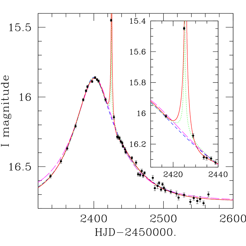
Figure 1.— The points with errorbars show the light curve of OGLE-2002-BLG-055. The long-dashed magenta line shows the best single-lens, single-source, constant-velocity model fit to the data, with the single high point and two neighboring points removed. The short-dashed blue line shows the best single-lens, single-source, constant-acceleration model fit to the same dataset. The dotted green line shows the best single-lens, binary-source, constant-acceleration model to the entire data set. The solid red line shows the best single-source, binary-lens, constant-acceleration model to the entire dataset. The inset shows a close-up near the deviation.

2. Data

The Galactic bulge microlensing event OGLE-2002-BLG-055 was observed as part of the third phase of the OGLE collaboration (Udalski, 2003b), and alerted during the 2002 bulge season with the Early Warning System (EWS). The OGLE data consist of 106 $I$-band data points, with 9 points taken during the 2001 season, 47 during the 2002 season, and 50 taken during the 2003 season. The data covering the primary event are shown in Figure 1. All errors are scaled by a factor of 1.31, as determined from the 2003 baseline data. This scaling may be somewhat underestimated, as the best models found here have unreasonably large values of $\chi^{2}$, although they appear to faithfully reproduce all the features of the event. The majority of the data for OGLE-2002-BLG-055 appear to follow the usual single-lens form, with the obvious exception of the data point at ${\rm HJD^{\prime}}\equiv{\rm HJD}-2450000.=2424.9$, which has $I=15.449\pm 0.009$, highly discrepant from the neighboring points at $I\sim 16$ separated by $4-8$ days. Jaroszyński & Paczyński (2002) report that this data point is secure, as evidenced by direct inspection of the raw image.

Unfortunately, there is only $I$-band data available for OGLE-2002-BLG-055, which hinders the interpretation of the model fits to the data for several reasons. First, without color information during the event, it is impossible to determine separately the color of the source and blend. Thus it is not possible to compare the derived source and blend colors and magnitudes to a local color-magnitude diagram, which provides an important test of the viability of a given model. In fact, as this field was not observed during the second phase of the OGLE collaboration, there is no $V$-band data available for the source field at all. Thus it is also not possible to determine the local $I$-band extinction $A_{I}$ via the usual method of ‘clump-calibration’ (Woźniak & Stanek, 1996; Stanek, 1996). There are several publicly-available extinction maps for the Galactic bulge. The maps of Sumi (2004) are based on OGLE II data, and thus do not cover the OGLE-2002-BLG-055 field. Popowski, Cook, & Becker (2003) have derived extinction maps based on MACHO collaboration data. We estimate the extinction at the location of the source (${\rm R.A.}=17^{\rm h}59^{\rm m}40.\hskip-2.0pt^{\rm s}93$, ${\rm Dec.}=-27^{\circ}07^{\prime}18.\hskip-2.0pt^{\prime\prime}2{\rm(J2000)}$; $l=3.14115,b=-1.75827$) as the mean of the two closest points (at distances of $0.12^{\circ}$ and $0.16^{\circ}$) in the Popowski, Cook, & Becker (2003) extinction maps, weighted by the inverse squared distance. This yields $A_{V}=3.20$, or $A_{I}=1.57$, where we have adopted $A_{I}/A_{V}=0.49$ (Udalski, 2003a; Sumi, 2004).

3. Modeling OGLE-2002-BLG-055: Technical Details

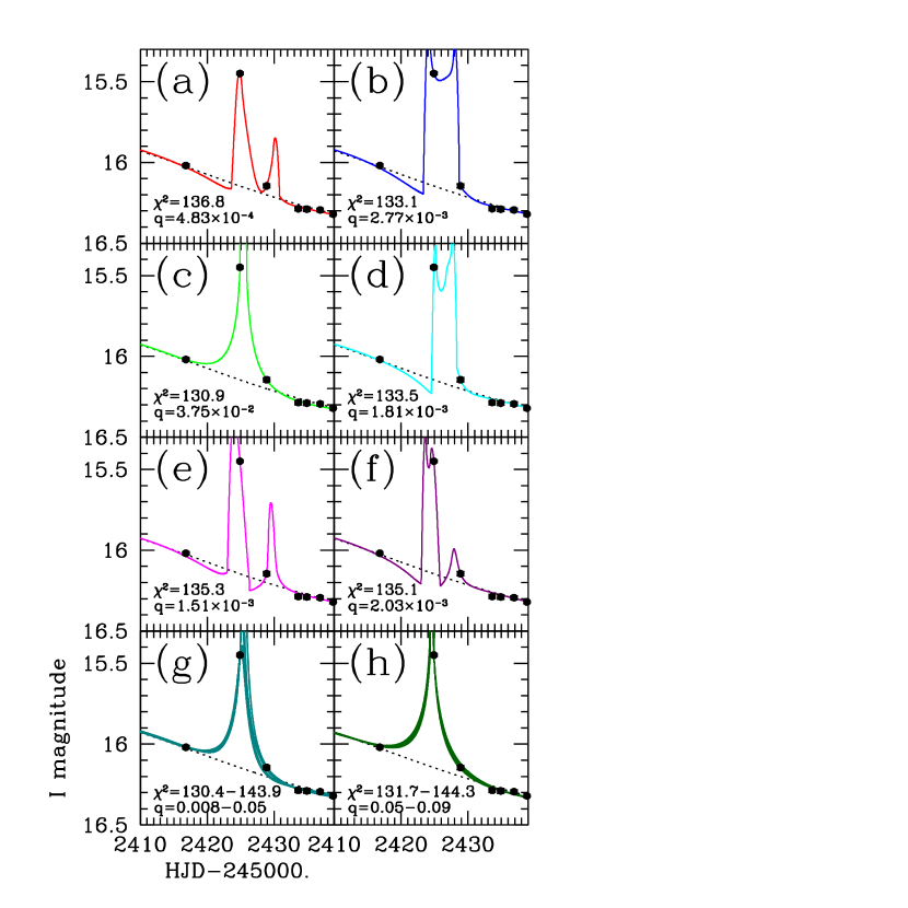
Figure 2.— In each panel, the points with errorbars show a close-up of the light curve of OGLE-2002-BLG-055 for $\sim 15$ days before and after the deviant data point. The solid curve in each panel shows a different single-source, binary-lens, constant-acceleration fit. The mass ratio and $\chi^{2}$ of each fit are also indicated. The dotted curve shows the best single-source, single-lens, constant-acceleration fit with three data points removed, and is the same as the dashed curve in Figure 1. The bottom two panels show a continuum of fits, with the range of mass ratios and $\chi^{2}$ values indicated.

We fit the flux as a function of time to the standard form,

$$F(t)=F_{s}A(t)+F_{b},$$ (1)

where $F_{s}$ is the flux of the source, and $F_{b}$ is the flux of any unrelated blended light. Here $A(t)$ is the magnification as a function of time $t$.

For a single lens (SL) and single source (SS), the magnification is,

$$A_{0}[u(t)]=\frac{u^{2}+2}{u\sqrt{u^{2}+4}}$$ (2)

where $u(t)$ is the angular separation between the lens and source in units of the angular Einstein ring radius,

$$\theta_{\rm E}=\sqrt{\kappa M\pi_{\rm rel}},\qquad\kappa=\frac{4G}{c^{2}{\rm AU}}.$$ (3)

Here $\pi_{\rm rel}$ is the lens-source relative parallax, and $M$ is the mass of the lens.

The angular separation between the source and lens can be written as,

$$u^{2}(t)=x^{2}(t)+y^{2}(t).$$ (4)

We consider two different models for the relative lens-source motion. For constant relative velocity (CV) between the source, lens, and observer,

$$x(t)=\tau\equiv\frac{t-t_{0}}{t_{\rm E}},\qquad y(t)=u_{0}$$ (5)

where $t_{\rm E}=\theta_{\rm E}/\mu_{\rm rel}$ is the Einstein timescale, $\mu_{\rm rel}$ is the relative lens-source proper motion, $t_{0}$ is the time of closest approach between lens and source, and $u_{0}$ is the impact parameter in units of $\theta_{\rm E}$. For constant acceleration (CA), the two components of the angular separation become (Smith, Mao, & Paczyński, 2003),

$$x(t)=\tau+\frac{1}{2}{\cal A}_{x}\tau^{2},\qquad y(t)=u_{0}+\frac{1}{2}{\cal A}_{y}\tau^{2}.$$ (6)

Here ${\cal A}_{x}$ and ${\cal A}_{y}$ are the two components of the relative source-lens angular acceleration in units of $\theta_{\rm E}/t_{\rm E}^{2}$. Note that $t_{\rm E}$ and $\mu_{\rm rel}$ are now defined at time $t_{0}$.

For a SL and binary source (BS), the magnification can be written

$$A_{\rm BS}(t)=A_{0}[u_{1}(t)]+\epsilon A_{0}[u_{2}(t)],$$ (7)

where $\epsilon$ is the flux ratio between the secondary and primary source. Here $u_{1}$ and $u_{2}$ are the angular separations between the primary and secondary source and the lens, respectively.

For a bound binary-source, we expand the vector angular separation of the primary and secondary around the time of maximum magnification of the primary $t_{0}$, and keep terms up to the acceleration. This yields $u_{1}(t)$ given by Eq. 6, with $t_{0}$ and $u_{0}$ the time of maximum magnification and impact parameter of the primary, and $u_{2}^{2}(t)=x_{2}^{2}(t)+y_{2}^{2}(t)$, with

$$x_{2}(t)=\tau_{1}-\frac{1}{2}\frac{{\cal A}_{x}}{q_{s}}\tau_{1}^{2}+b_{x},\qquad y_{2}(t)=u_{0}-\frac{1}{2}\frac{{\cal A}_{y}}{q_{s}}\tau_{1}^{2}+b_{y},$$ (8)

where $\tau_{1}=(t-t_{0})/t_{\rm E}$, and $q_{s}$ is the mass ratio of the binary-source system, and ${\bf b}=(b_{x},b_{y})$ is the vector angular separation from the primary to the secondary in units of $\theta_{\rm E}$, which has the same direction as the acceleration of the primary. Unfortunately, this parameterization is not ideal for the current event because $b_{x}$ and $b_{y}$ are not directly constrained by the data, but rather the magnification of the secondary source at the time of the deviant data point, $A(t_{d})\simeq\epsilon/u_{2}(t_{d})$. Therefore, adopting Eq. 8 would lead to correlations between the parameters ${\cal A}_{x},{\cal A}_{y},t_{0},u_{0}$, $b_{x}$, and $b_{y}$, which would lead to complications with fitting and error determination. Instead, we adopt $x_{2}(t)=(t-t_{0,2})/t_{\rm E}$ and $y_{2}(t)=u_{0,2}$. This assumes that the acceleration of the secondary is negligible, and that the direction of the acceleration of the primary is not necessarily the same as ${\bf b}$. The acceleration of the secondary has two effects. First, the effective timescale at the time of the perturbation may be different from $t_{\rm E}$. Second, the deviation from uniform velocity induces a deviation in the light curve. The former effect is essentially unobservable, because the difference in $t_{\rm E}$ can be absorbed into $\epsilon$ and $u_{0,2}$ (Gould, 1996; Gaudi, 1998). For typical parameters, the deviation in the light curve due to acceleration is $\lesssim 1\%$ while the magnification of the secondary is significant. This is of order or smaller than the errors, and thus is negligible. The alignment between the source separation vector and acceleration vector as determined from the fit provides an important test of the binary-source interpretation.

For a binary lens (BL), the magnification is specified by three parameters: the mass ratio $q$ of the lens, and instantaneous angular separation $d$ between the two components in units of $\theta_{\rm E}$, and the angle $\alpha$ between the vector pointing from primary to secondary and the direction of $\mu_{\rm rel}$. Here we adopt a coordinate system such that the origin of the binary-lens is at a distance of $qd^{-1}(1+q)^{-1}$ from the primary along the axis toward the secondary. For BL models with small mass ratios, it is also necessary to consider the effect the finite size of the source star $\theta_{*}$ on the magnification, parameterized by $\rho_{*}\equiv\theta_{*}/\theta_{\rm E}$.

We perform all fits in flux rather than magnitude space, thus allowing the analytic determination of the values of $F_{s}$ and $F_{b}$ for a given model $A(t)$ that minimize the usual $\chi^{2}$ goodness-of-fit statistic. All other parameters are minimized using the downhill-simplex routine AMOEBA (Press, Teukolsky, Vetterling, & Flannery, 1992), using many different initial trial values of the parameters as seeds. This procedure works well for all models except the BL model, which generally produces poorly-behaved $\chi^{2}$ surfaces that are not well explored by downhill-simplex routines.

In order to approximately minimize BL models, and to calculate errors on fit parameters for other models, we use a Markov Chain Monte Carlo (MCMC). At each step in the chain, we vary a single fit parameter by drawing a random Gaussian deviate with zero mean, and dispersion set to appropriately sample the likelihood surface. We then calculate the relative likelihood ${\cal L}_{rel}=\exp(-\Delta\chi^{2}/2)$ between the new step, and the old position. If ${\cal L}_{rel}\geq 1$, the step is accepted. If ${\cal L}_{rel}<1$, then we draw a random uniform deviate between 0 and 1. If this deviate is $<{\cal L}_{rel}$, then the new step is accepted, otherwise it is rejected. When generated in this way, the resulting distribution of parameters in the Markov Chain is proportional to the posterior probability distribution, provided that the chain has converged. Although we do not rigorously test for convergence, we confirm that the chains have been run for a sufficient number of steps, by visually inspecting different chains started at different points in parameter space, and ensuring that these have properly mixed.

We define the $1\sigma$ errors on a given parameter as the projection of the $\Delta\chi^{2}=1$ contour onto that parameter axis. We do not attempt to calculate errors for the BL models, primarily because we find that there are large, disconnected regions of parameter space that contain continua of degenerate models. Defining confidence regions in the presence of such degeneracies is difficult and not very meaningful.

4. Modeling OGLE-2002-BLG-055: Results

Table 1 shows fit parameters and, where appropriate, $1\sigma$ errors for the four different classes of models considered here. The models are labeled by the lens multiplicity (SL=single lens, BL=binary lens), source multiplicity (SS=single source, BS=binary source), and source motion (CV=constant velocity, CA=constant acceleration). Also indicated is the dataset used; no number refers to the entire dataset, ‘1’ indicates the dataset with the single deviant data point at $t_{d}=2424.9$ removed, ‘3’ refers the dataset with points at $t=2416.81$, $2424.9$, and $2428.89$ removed. For the constant acceleration fits, there are generally always two degenerate models (Smith, Mao, & Paczyński, 2003), these are labeled ‘p’ and ‘n’ for the fits with positive and negative ${\cal A}_{y}$, respectively. The binary-lens fits are labeled as (a,b,c,d,e,f), which correspond to the panel labels in Figure 2.

Following Jaroszyński & Paczyński (2002), we first fit OGLE-2002-BLG-055 to a standard single-lens, single-source, constant velocity model after removing the single deviant data point at $t_{d}=2424.9$. This model is clearly a poor fit to the data, yielding $\chi^{2}\simeq 180$ for 100 degrees of freedom (dof). Removing two additional data points on either side of the deviant data point improves the fit by $\Delta\chi^{2}=12$ for two fewer dof. This implies that the two data points on either side of the point at $t_{d}$ likely deviate significantly from the smooth underlying model, supporting the reality of the single data point, and pointing toward a perturbation that has a timescale that is of order the interval between the $t_{d}$ and neighboring data points, $\sim 4~{}{\rm days}$. All constant-velocity fits are quite poor, deviating significantly from the data during the rising part of the primary event (see Figure 1), likely indicating a significant acceleration of the observer, source, or lens.

Including a constant acceleration improves the fits considerably. For the data set with one data point removed, we find $\chi^{2}\simeq 149$ for 98 dof. When three data points are removed, the fit improves by $\Delta\chi^{2}=15.7$ for 2 less degrees of freedom. As anticipated by Smith, Mao, & Paczyński (2003), we find two degenerate fits for each constant acceleration model, with different values of $t_{\rm E}$, ${\cal A}_{x}$, and ${\cal A}_{y}$, but identical values of the other parameters and $\chi^{2}$. Including the constant acceleration terms increases the inferred timescale considerably. The value of $\chi^{2}$ for the best-fit constant acceleration model with three data points removed is unacceptably high, despite the fact that the model appears to reproduce the primary features of dataset quite well (see Figure 1). Inspection of the light curve during the microlensing event, while the source is significantly magnified, reveals short timescale ($\lesssim 1~{}{\rm day}$) scatter, with amplitude that is smaller than the typical size of the photometric errors at baseline. This scatter may be intrinsic to the source. Regardless of the cause, it appears that the error scaling derived from the baseline points is probably underestimated.

A binary-source model can produce a large, short-timescale deviation like that seen in the dataset of OGLE-2002-BLG-055, provided that $\epsilon\ll 1$ and $u_{0,2}\ll 1$. Figure 2 shows the best-fit binary-source models, which have $\chi^{2}\simeq 142$ for 96 degrees-of-freedom. This is $\Delta\chi^{2}\simeq 11$ larger than the single-source constant-acceleration fit with three data points removed. This additional $\chi^{2}$ arises from the inability of the binary-source model to simultaneously fit the two data points immediately following $t_{d}$. As with the single-source models, there are two binary-source models with essentially equal $\chi^{2}$ due to the constant-acceleration degeneracy. As anticipated, the fits yield small values for the flux ratio, $\epsilon\simeq 1\%$. In this regime, the relations between the binary-source parameters $\epsilon,u_{0}$, and $t_{0}$ and the salient features of the perturbation are exceedingly simple (Gaudi, 1998). Note that the parameters of the primary ($t_{0},t_{\rm E},u_{0},{\cal A}_{x},{\cal A}_{y},F_{s},F_{b}$), which are constrained by the data away from the perturbation, are essentially identical to the parameters found for the constant-acceleration fits with three data points removed. The duration of the perturbation is constrained by the points neighboring $t_{d}$. Combined with the parameters of the primary, this duration yields $\epsilon$. The excess flux at time $t_{d}$ is $\Delta F(t_{d})\simeq F_{s}\epsilon/u_{2}(t_{d})$, and thus yields $u_{2}(t_{d})$, which is much better constrained than $t_{0,2}$ and $u_{0,2}$ separately. We find $u_{2}(t_{d})=0.0025\pm 0.0008$ and $u_{2}(t_{d})=0.0018\pm 0.0007$ for models SL.BS.CA.n and SL.BS.CA.p, respectively. Note that, since the relations between the perturbation observables and the binary-source parameters $\epsilon,t_{0,2},u_{0,2}$ depend on $t_{\rm E}$, which differs between the two constant-acceleration fits, the binary-source parameters also differ between the two fits.

Binary-lens models with extreme mass ratios $q$ can also yield large, short-timescale deviations. In the limit of $q\ll 1$, and under some simplifying assumptions, the relation between the gross features of the perturbation and the binary parameters $q,d,\alpha$ also take on a relatively simple form (Gould & Loeb, 1992; Gaudi & Gould, 1997). The angle of the trajectory is roughly $\alpha\sim\tan^{-1}[{u_{0}/\tau(t_{d})}]$. The binary separation is $d\sim 0.5[u_{d}+\sqrt{u_{d}^{2}+4}]$, where $u_{d}=\sqrt{\tau(t_{d})^{2}+u_{0}^{2}}$. Finally, the mass ratio is $q\sim\sqrt{\Delta t/t_{\rm E}}$. For fits SL.SS.CA.3n and SL.SS.CA.3p, these expressions yield $\alpha\sim 0.6-0.8$, $d\sim 1.1$, and $q\sim 10^{-3}$. Of course, these formulas are only very rough approximations, but the implied parameters are good starting guesses. We therefore start with these parameter ranges, and first alter the parameters by hand until we find a number of promising approximate fits. These fits are then used as seeds for an automated point-source binary-lens minimization routine. All viable point-source fits are then collected, and the parameters are used as starting guesses for a second minimization, using a finite source of angular size

$$\theta_{*}=6~{}{\mu{\rm as}}~{}10^{-0.2(I_{0}-14.32)}.$$ (9)

Here $I_{0}$ is the dereddened magnitude of the source as derived from the point-source fits. Equation (9) is derived from the color-surface brightness relation of van Belle (1999), assuming that the $(V-I)_{0}$ color of the source is the same as the red clump. Standard models of the Galaxy (Han & Gould, 1995, 2003) predict $\left<\theta_{\rm E}\right>=240^{+190}_{-130}{\mu{\rm as}}$ (bulge), and $\left<\theta_{\rm E}\right>=330^{+360}_{-190}{\mu{\rm as}}$ (disk). These values of $\theta_{\rm E}$ yield source sizes $\rho_{*}=\theta_{*}/\theta_{\rm E}$ that are too large to reproduce the data for OGLE-2002-BLG-055 with small mass ratios $q$. Although this implies that such fits are somewhat disfavored, it is not actually possible to rule out these models with such an argument. We therefore adopt a value of $\theta_{\rm E}=550{\mu{\rm as}}$. Approximately $6\%$ of bulge lenses and $25\%$ of disk lenses are expected to have values of $\theta_{\rm E}$ larger than this.

Representative finite-source, binary-lens fits are tabulated in Table 1 and shown in Figure 2. We recover the fits presented by Jaroszyński & Paczyński (2002), and find many other additional viable fits, with mass ratios ranging from $q\simeq 5\times 10^{-4}$ to $\sim 8\times 10^{-2}$, at the $\Delta\chi^{2}\lesssim 9$ level. The best binary-lens (and best overall) fit has $\chi^{2}=130$ for 96 dof. If one forces $\chi^{2}/{\rm dof}=1$ for this fit, then mass ratios in the range $q=10^{-4}-10^{-2}$ are all consistent with the data at the $\sim 3\sigma$ level.

There two basic classes of fits. In the first class the trajectory crosses the planetary caustic, with the deviant data point at $t_{d}$ occurring when the source is interior to, or near, the caustic. The second class of fits pass outside the planetary caustic, with the point at $t_{d}$ occurring when the source is near the ridge of high-magnification on the planet-star axis. The second class actually represents a continuous degeneracy in $q,d$, and $\alpha$, with mass ratios in the range $0.01\lesssim q\lesssim 0.1$ for $\Delta\chi^{2}\lesssim 14$. From Figure 2, we conclude that while many of the fits would have been distinguishable with a few additional data points during the perturbation, the family of continuous fits produce very similar perturbations. The curves in each of the two bottom panels of Figure 2 deviate from each other by $\lesssim 2\%$ for the majority of the perturbation. Distinguishing between these models would therefore require rather accurate or densely sampled data. The cause of this uncertainty in $q$ is briefly discussed by (Gaudi & Gould, 1997).

5. Implications and Discussion

OGLE-2002-BLG-055 can be reasonably well-fit by large number of different models. Jaroszyński & Paczyński (2002) demonstrated that the asymmetry exhibited by the primary light curve can be explained by a simple uniform acceleration, due to either parallax deviations arising from the motion of the Earth, or non-uniform motion of the source due to the presence of, e.g., a binary companion. We have demonstrated that the short-timescale deviation can be explained by a binary companion to the lens with mass ratio $10^{-4}\lesssim q\lesssim 10^{-1}$, consistent with a planet, brown dwarf, or low mass star. The short-timescale deviation can also be explained by a binary companion to the source with a flux ratio of $\sim 1\%$.

Which of these models is most likely? Jaroszyński & Paczyński (2002) showed that the parallax and constant acceleration fits had essentially identical $\chi^{2}$-values for the same number of degrees-of-freedom. Thus either are equally viable in a goodness-of-fit sense. The inferred timescale of the event spans the range $t_{\rm E}=50-100~{}{\rm days}$, which is in the range where weak parallax effects are neither surprising, nor necessarily expected. Furthermore, there has been no estimation of the expected rate of binary-source events with detectable asymmetries due to acceleration. Therefore it is difficult to argue which origin for the observed asymmetry is a priori more likely. In regards to the deviant data point, a binary-lens model with $q\sim{\rm few}\times 10^{-2}$ provides the best fit to the data, with the binary-source model disfavored at $\Delta\chi^{2}=11$ for the same number of dof, or slightly more than $\sim 3\sigma$ level. However, this difference in $\chi^{2}$ is driven primary by a couple of data points just after the perturbation, which may be affected by the short-timescale variability seen in other parts of the light curve. If one normalizes the error bars to force $\chi^{2}/{\rm dof}=1$ for the best model, then the binary-lens model is only favored at the $\Delta\chi^{2}\simeq 8$ level. The inferred blend and source fluxes can also provide discrimination between models: one expects these fluxes to trace, on average, the distribution of fluxes of unlensed stars in the field near the line-of-sight. The best binary-lens models have source and blend magnitudes of $I_{s}\sim 17$ and $I_{b}\sim 19$, whereas the binary-source fits yield $I_{s}\sim 18$ and $I_{b}\sim 17$. Unfortunately, without color information, it is difficult to definitively distinguish between these two scenarios. It is also difficult to argue which model is a priori more likely, since the frequency of planetary companions to microlens stars is not known, and defining the appropriate detection criterion for the current event, which was culled by eye from an ensemble of alerted microlensing events, is nebulous at best.

The binary-source model does have the advantage of simplicity: a bound companion to the primary source can explain both the short-timescale variability and the acceleration needed to produce the global asymmetry. However, in order for this scenario to hold, the projected acceleration vector must be aligned with the projected binary-source separation vector. In the particular parameterization of the binary-source model used here (see §3), this angle $\Delta\theta$ between the two vectors is essentially a free parameter, and thus it can be used to test the model. We determine the distribution of $\Delta\theta$ from the two Markov chains corresponding to the two degenerate (in the sense of $\chi^{2}$) binary-source models, SL.BS.CA.n and SL.BS.CA.p. The second model is immediately ruled out, as the primary’s acceleration vector is pointing away from the companion, with $\Delta\theta>90^{\circ}$, wildly inconsistent with any bound orbit. The first model has $\Delta\theta=36.2_{-2.0}^{+1.8}$ degrees. At first sight, this may also seem very inconsistent ($>15\sigma$!) with a bound orbit ($\Delta\theta=0$), however there are several reasons why this is not necessarily correct. First, although the $1\sigma$ uncertainty on $\Delta\theta$ is small, there is a substantial non-Gaussian tail toward smaller values. Enforcing $\Delta\theta=0$ in the fit yields $\chi^{2}=156.7$, or $\Delta\chi^{2}=15.0$ for one less dof. Thus, the bound model is only ‘ruled out’ at the $\sim 3.5\sigma$ level. Furthermore, as we argue below, the period of a bound binary source with separation $b\lesssim 1$ is likely to be only a few times longer than the timescale of the event. Therefore one expects significant deviations from uniform acceleration that are not accounted for in the simplified model adopted here. Thus the inferred value of the $\Delta\theta$ may be the result of inadequacies in the model. It is therefore conceivable OGLE-2002-BLG-055 could be fit by a bound binary-source model in which the effects of rotation are included self-consistently.

Accepting the binary-source model as correct, one can use the measured parameters of the viable model SL.BS.CA.n to determine the Einstein ring radius projected on the source plane $\hat{r}_{\rm E}=D_{\rm os}\theta_{\rm E}$ (Han & Gould, 1997), where $D_{\rm os}$ is the distance to the lens. Assuming circular orbits, the acceleration of the primary due to the secondary is simply $a=Gm_{2}/d^{2}$, where $d$ is the semi-major axis of the orbit and $m_{2}$ is the mass of the secondary. The projected acceleration $a_{\perp}$ is therefore,

$$a_{\perp}=\frac{Gm_{2}}{d^{2}}(1-\sin^{2}{\phi}\sin^{2}{i})^{1/2}$$ (10)

where $i$ is the inclination of the orbit, and $\phi$ is the phase of the primary orbit referenced to the intersection of the orbit and the plane of the sky. The constant-acceleration fit yields the parameter ${\cal A}=\sqrt{{\cal A}_{x}^{2}+{\cal A}_{y}^{2}}$, which is given by,

$${\cal A}=\frac{a_{\perp}t_{\rm E}^{2}}{\hat{r}_{\rm E}}.$$ (11)

The binary-source fit yields $t_{0,2}$. This can be combined with the parameters of the primary event to derive the two components the projected binary-source separation: $b_{x}=0.5({\cal A}_{x}/q_{s})\Delta\tau^{2}-\Delta\tau$ and $b_{y}=0.5({\cal A}_{y}/q_{s})\Delta\tau^{2}-u_{0}$. Here $\Delta\tau\equiv(t_{0,2}-t_{0})/t_{\rm E}$, and we have assumed that $u_{0,2}\ll 1$. Then $b$ can be related to the semi-major axis by,

$$d=\hat{r}_{\rm E}b(\cos^{2}{\phi}+\cos^{2}{i}\sin^{2}{\phi})^{-1/2}.$$ (12)

Finally, Equations (10), (11), and (12) can be combined to arrive at an expression for $\hat{r}_{\rm E}$ in terms of mostly known quantities,

$$\hat{r}_{\rm E}=\left[\frac{Gm_{2}t_{\rm E}^{2}}{b^{2}{\cal A}}(1-\sin^{2}{\phi}\sin^{2}{i})^{1/2}(\cos^{2}{\phi}+\cos^{2}{i}\sin^{2}{\phi})\right]^{1/3}.$$ (13)

We now use the probability distribution of the binary-source model fit parameters, together with equation (13), to construct the probability distribution for $\hat{r}_{\rm E}$. Here the virtue of MCMC becomes clear: in order to determine the probability distribution of $\hat{r}_{\rm E}$, we simply have to determine the value of $\hat{r}_{\rm E}$ at each link in the chain. Because the density of points in the binary-source MCMC parameter chain is proportional to the posteriori probability distribution, the resulting distribution of values of $\hat{r}_{\rm E}$ is simply proportional to the desired probability distribution.

We first account for the parameters in equation (13) that are not constrained by the binary-source model; these include the inclination $i$, the phase $\phi$, and the mass ratio $q_{s}$ (which enters via $b$). For each link in the chain, we randomly choose ten values of $\phi$ and $\cos{i}$, assuming a uniform distribution of each. We determine $q_{s}$ using the fluxes of the primary and the secondary. We draw a source distance $D_{\rm os}$ from the standard Galactic model of Han & Gould (1995, 2003). If the source is in the bulge, we assume that the primary is a giant, and therefore has a mass of $M_{1}\sim M_{\odot}$. If the source is in the disk, we determine the absolute magnitude of the primary from the value of $D_{\rm os}$, and assuming an extinction of $A_{I}=1.57$ (see §2). We determine the absolute magnitude of the secondary from the flux ratio $\epsilon$, primary flux $F_{s}$, $D_{\rm os}$, and $A_{I}$. We estimate the masses of the primary and secondary from their absolute magnitudes using an analytic approximation to the main-sequence mass-luminosity relationship derived from the solar metallicity isochrones of Bertelli et al. (1994). This then yields the mass ratio $q_{s}$. We then determine $\hat{r}_{\rm E}$.

In addition, we also determine the radius $R_{*,2}$ of the secondary from its absolute magnitude, also using the solar-metallicity isochrones of Bertelli et al. (1994). We require that $\rho_{*,2}\equiv R_{*,2}/\hat{r}_{\rm E}<u_{2}(t_{d})$, otherwise we discard the inferred value of $\hat{r}_{\rm E}$. We note that the resulting distribution of $\hat{r}_{\rm E}$ is not very sensitive to the adopted distribution of source distances, for several reasons. First, the distance enters through the factor of $b^{-2/3}$, since $b$ formally depends on the mass ratio $q_{s}$. However, inspection of the expressions for $b_{x}$ and $b_{y}$ reveals that $q_{s}$ modifies the acceleration terms, which themselves are $\propto\tau_{2}^{2}$, where $\tau_{2}=(t_{0,2}-t_{0})/t_{\rm E}$. For the binary-source fits presented here, $\tau_{2}^{2}\sim 10\%$, and thus these terms are small. Second, for bulge sources, where $q_{s}$ is affected the most by the assumed source distance, the dispersion in source distances is relatively small. Conversely, for disk sources, where the dispersion in source distances is large, the inferred value of $q_{s}$ is relatively insensitive to the source distance (since both primary and secondary are assumed to be on the main sequence). Had we simply assumed that all sources were in the bulge with $D_{\rm os}=8~{}{\rm kpc}$, the median inferred value of $\hat{r}_{\rm E}$ would change by $\lesssim 2\%$, or $\sim 0.1\sigma$.

Figure 3 shows the resulting distribution of $\hat{r}_{\rm E}$. The median and 68% confidence interval is $\hat{r}_{\rm E}=1.87\pm 0.40~{}{\rm AU}$. Adopting the standard Galactic model of Han & Gould (1995, 2003), we use the inferred values of $\hat{r}_{\rm E}$ and $t_{\rm E}$ to constrain the mass $M$, distance $D_{\rm ol}$ and relative proper motion $\mu_{\rm rel}$ of the lens. The resulting distribution of $M$ (assuming a uniform prior in linear mass) is shown in Figure 3. The median and $68\%$ confidence interval is $\log{M/M_{\odot}}=-0.28_{-0.42}^{+0.58}$. Similarly, we infer $D_{\rm ol}=7.1\pm 0.9~{}{\rm kpc}$, $\theta_{\rm E}=240_{-40}^{+45}\mu{\rm as}$, and $\mu_{\rm rel}=5.45_{-0.95}^{+1.15}~{}{\rm km~{}s^{-1}~{}kpc^{-1}}$. All of these parameters are typical for disk-bulge or bulge-bulge lensing events, except for $\mu_{\rm rel}$, which is a factor of $\sim 6$ smaller than the median distribution for bulge-bulge events and a factor of $\sim 8$ smaller than the median of disk-bulge events. This may be due to the fact that the lens and source happen to have usually small relative velocities, it may indicate that the event is due to disk-disk lensing, or it may simply be because the model is incorrect.

We also infer an Einstein ring radius projected onto observer plane of $\tilde{r}_{\rm E}=13.3_{-7.0}^{+15.5}~{}{\rm AU}$, indicating that, for the binary-source model, parallax effects are likely to be negligible.

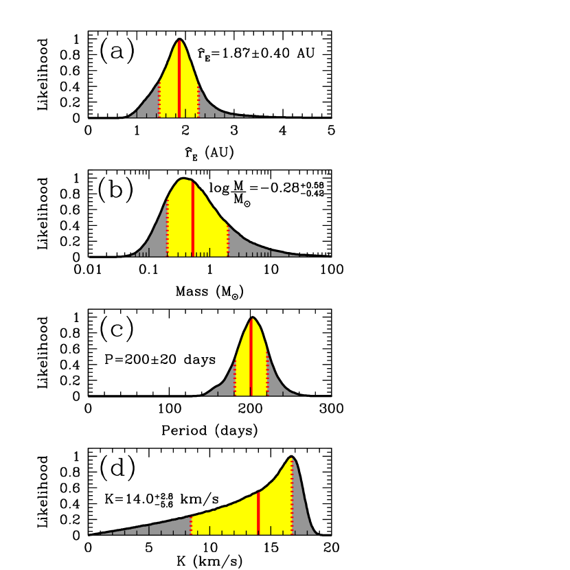
Figure 3.— In each panel, the curves show the relative likelihood of the given parameter, as inferred from binary-source, constant acceleration fit SL.BS.CA.n (see Table 1 and §5). All curves have been normalized so that the likelihood is unity at the peak. The solid vertical line shows the median of the distribution, while the dotted lines show the 68% confidence limits. (a) The relative likelihood of $\hat{r}_{\rm E}$, the Einstein ring radius of the lens projected on the source place. (b) The relative likelihood of the mass of the lens, as inferred from the measured values of $\hat{r}_{\rm E}$, the timescale $t_{\rm E}$, and the standard Galactic model of Han & Gould (1995, 2003). (c) The relative likelihood of the period of the binary-source in days. (c) The relative likelihood of the semi-amplitude $K$ of the radial velocity of the primary of the binary source, in kilometers per second.

The probability distributions of several other interesting quantities can also be constructed from the Markov chain. The semi-major axis of the binary is $d=0.80\pm 0.06~{}{\rm AU}$. In order to determine the period, we assume a primary mass of $m_{1}=M_{\odot}$, as expected for bulge giants. The absolute $I$-band magnitude of the secondary is $M_{I}=6.60\pm 0.46$, which corresponds to a mass of $m_{2}=0.67\pm 0.05~{}M_{\odot}$ assuming that it is on the main-sequence. These corresponds to a late K-dwarf. The primary has an absolute magnitude of $M_{I}=2.01\pm 0.49$, making it likely to be a $M_{1}\sim M_{\odot}$ bulge giant. The total binary mass is $M_{s}\equiv m_{1}+m_{2}\simeq 1.7M_{\odot}$. The distribution of the binary period is shown in Figure 3, the median and 68% confidence interval is $P=200\pm 20~{}{\rm days}$. The binary period is only a factor of $\sim 2$ larger than the microlensing event timescale $t_{\rm E}$. This implies that the assumption of a uniform acceleration is almost certainly violated, and that the binary-source model is not internally self-consistent. The constant acceleration approximation may not be so bad, as the deviations from uniform acceleration will only become significant in the tails of the event, when it is not highly magnified. Nevertheless, the parameters derived from the above analysis should be interpreted with caution.

It is also possible to predict the semi-amplitude of the radial velocity of the primary,

$$K=\left[\frac{Gm_{2}^{2}}{dM_{\rm s}}\right]^{1/2}\sin{i}.$$ (14)

The distribution of $K$ is shown in Figure 3. The median and 68% confidence interval is $14.0_{-5.6}^{+2.8}~{}{\rm km~{}s^{-1}}$. Radial velocity precisions of a few ${\rm km~{}s^{-1}}$ should be attainable for this source, which has $I=17.9$. Thus it may be possible to directly confirm the binary-source interpretation of this event.

6. Conclusion

Microlensing event OGLE-2002-BLG-055 exhibits a slightly asymmetric, smooth light curve with a single data point that deviates by $\sim 0.6$ magnitudes from neighboring points separated by several days. Jaroszyński & Paczyński (2002) concluded that the simplest interpretation of OGLE-2002-BLG-055 was an event with parallax deviations arising from the motion of the Earth, and a short-timescale deviation due to a binary lens with mass ratio $q=10^{-3}-10^{-2}$, thereby making OGLE-2002-BLG-055 a candidate planetary event.

Here we demonstrated that OGLE-2002-BLG-055 can be reasonably well-fit by several different classes of models, and a wide range of parameters within each model class. We found that the data can be fit by many different binary-lens models whose mass ratios span three orders of magnitude, from $q=10^{-4}$ to $10^{-1}$, thereby making the secondary consistent with a planet, brown dwarf, or M-dwarf for reasonable primary masses. A subset of these binary-lens fits form a family of continuously degenerate models, whose mass ratios differ by an order of magnitude. Astonishingly, the light curves of these models differ by $\lesssim 2\%$ for the majority of their duration. A binary-source model is also consistent with the data, for a secondary/primary flux ratio of $\sim 1\%$. This model also naturally explains the global asymmetry of the lightcurve as due to the acceleration of the primary induced by the secondary. Under the assumption of a bound binary-source, this model yields an estimate of the Einstein ring radius projected on the source plane of ${\hat{r}_{\rm E}}=1.87\pm 0.40~{}{\rm AU}$.

All of these fits differ by $\lesssim 3\sigma$, and are essentially indistinguishable when the scatter due to likely source variability is considered. Unfortunately, the lack of color information during the event precludes the discrimination of models based on the positions of the source and blend on a color-magnitude diagram.

Although the primary goal of the study by Jaroszyński & Paczyński (2002) was to affect a modification of the OGLE observation strategy to ensure good sampling of short-duration perturbations, rather than argue that OGLE-2002-BLG-055 was a bona fide planetary event, it is still somewhat disturbing that many binary-lens fits were missed, and the possibility of a binary-source interpretation was not discussed at all. OGLE-2002-BLG-055 serves as an extreme reminder of the degeneracies inherent in microlensing events, and highlights the difficulties in interpreting poorly-sampled and weakly-perturbed events. These difficulties become especially important when attempting to detect planets with microlensing. Here observers and modelers need to be especially vigilant: in order to produce convincing and reliable planetary detections, it is essential not only to achieve dense and accurate photometry of planetary perturbations, but also to acquire as much auxiliary information as possible, and to perform detailed, careful, and thorough modeling, in order to ensure that planetary detections are robust.

References

- Afonso et al. (2000) Afonso, C., et al. 2000, ApJ, 532, 340
- Albrow et al. (1999) Albrow, M. D., et al. 1999, ApJ, 522, 1022
- Albrow et al. (2000) Albrow, M. D. et al. 2000, ApJ, 534, 894
- Albrow et al. (2002) Albrow, M. D., et al. 2002, ApJ, 572, 1031
- Bennett et al. (1999) Bennett, D. P. et al. 1999, Nature, 402, 57
- Bertelli et al. (1994) Bertelli, G., Bressan, A., Chiosi, C., Fagotto, F., & Nasi, E. 1994, A&AS, 106, 275
- Collinge (1994) Collinge, M.J. 2004 (astro-ph/0402385)
- Park et al. (2004) DePoy, D. L. et al. 2004, ApJ, submitted (astro-ph/0401250)
- Dominik (1998) Dominik, M. 1998, A&A, 333, 893
- Dominik (1999) Dominik, M. 1999, A&A, 349, 108
- Gaudi (1998) Gaudi, B. S. 1998, ApJ, 506, 533
- Gaudi & Gould (1997) Gaudi, B. S. & Gould, A. 1997, ApJ, 486, 85
- Gaudi et al. (2002) Gaudi, B. S. et al. 2002, ApJ, 566, 463
- Gould (1992) Gould, A. 1992, ApJ, 392, 442
- Gould (1996) Gould, A. 1996, ApJ, 470, 201
- Gould (2003) Gould, A. 2003, ApJ, submitted (astro-ph/0311548)
- Gould & Loeb (1992) Gould, A. & Loeb, A. 1992, ApJ, 396, 104
- Gould, Miralda-Escudé, & Bahcall (1994) Gould, A., Miralda-Escudé, J., & Bahcall, J. N. 1994, ApJ, 423, L105
- Griest & Hu (1992) Griest, K. & Hu, W. 1992, ApJ, 397, 362
- Griest & Safizadeh (1998) Griest, K., Safizadeh, N. 1998, ApJ, 500, 37
- Han (2002) Han, C. 2002, ApJ, 564, 1015
- Han & Gould (1995) Han, C. & Gould, A. 1995, ApJ, 447, 53
- Han & Gould (1997) Han, C. & Gould, A. 1997, ApJ, 480, 196
- Han & Gould (2003) Han, C. & Gould, A. 2003, ApJ, 592, 172
- Han & Jeong (1998) Han, C. & Jeong, Y. 1998, MNRAS, 301, 231
- Jaroszyński & Mao (2001) Jaroszyński, M. & Mao, S. 2001, MNRAS, 325, 1546
- Jaroszyński & Paczyński (2002) Jaroszyński, M. & Paczyński, B. 2002, Acta Astronomica, 52, 361
- Mao & Di Stefano (1995) Mao, S. & Di Stefano, R. 1995, ApJ, 440, 22
- Mao & Paczyński (1991) Mao, S. & Paczyński, B. 1991, ApJ, 374, L37
- Paczyński (1986) Paczyński, B. 1986, ApJ, 304, 1
- Popowski, Cook, & Becker (2003) Popowski, P., Cook, K. H., & Becker, A. C. 2003, AJ, 126, 2910
- Press, Teukolsky, Vetterling, & Flannery (1992) Press, W. H., Teukolsky, S. A., Vetterling, W. T., & Flannery, B. P. 1992, Numerical Recipes(Cambridge: Cambridge University Press)
- Smith et al. (2002) Smith, M. C. et al. 2002, MNRAS, 336, 670
- Smith, Mao, & Paczyński (2003) Smith, M. C., Mao, S., & Paczyński, B. 2003, MNRAS, 339, 925
- Stanek (1996) Stanek, K. Z. 1996, ApJ, 460, L37
- Sumi (2004) Sumi, T. 2004, MNRAS, 349, 193
- Udalski (2003a) Udalski, A. 2003a, ApJ, 590, 284
- Udalski (2003b) Udalski, A. 2003b, Acta Astronomica, 53, 291
- van Belle (1999) van Belle, G. T. 1999, PASP, 111, 1515
- Verde et al. (2003) Verde, L. et al. 2003, ApJS, 148, 195
- Woźniak & Stanek (1996) Woźniak, P. R. & Stanek, K. Z. 1996, ApJ, 464, 233