$K$-band Properties of Galaxy Clusters and Groups:
Luminosity Function, Radial Distribution and Halo Occupation Number

Abstract

We explore the near-infrared (NIR) $K$-band properties of galaxies within 93 galaxy clusters and groups using data from the Two Micron All Sky Survey (2MASS). We use X-ray properties of these clusters to pinpoint cluster centers and estimate cluster masses. By stacking all these systems, we study the shape of the cluster luminosity function and the galaxy distribution within the clusters. We find that the galaxy profile is well described by the NFW profile with a concentration parameter $c\sim 3$, with no evidence for cluster mass dependence of the concentration. Using this sample, whose masses span the range from $3\times 10^{13}M_{\odot}$ to $2\times 10^{15}M_{\odot}$, we confirm the existence of a tight correlation between total galaxy NIR luminosity and cluster binding mass, which indicates that NIR light can serve as a cluster mass indicator. From the observed galaxy profile, together with cluster mass profile measurements from the literature, we find that the mass–to–light ratio is a weakly decreasing function of cluster radius, and that it increases with cluster mass. We also derive the mean number of galaxies within halos of a given mass, the halo occupation number. We find that the mean number scales as $N\propto M^{0.84\pm 0.04}$ for galaxies brighter than $M_{K}=-21$, indicating high mass clusters have fewer galaxies per unit mass than low mass clusters. Using published observations at high redshift, we show that higher redshift clusters have higher mean occupation number than nearby systems of the same mass. By comparing the luminosity function and radial distribution of galaxies in low mass and high mass clusters, we show that there is a marked decrease in the number density of galaxies fainter than $M_{*}$ as one moves to higher mass clusters; in addition, extremely luminous galaxies are more probable in high mass clusters. We explore several processes– including tidal interactions and merging– as a way of explaining the variation in galaxy population with cluster mass.

1 Introduction

Understanding galaxy formation is one of the most outstanding challenges in cosmology. The development of both semianalytic (e.g. White & Rees 1978; Kauffmann et al. 1993; Cole et al. 2000, among others) and numerical (e.g. Kauffmann et al. 1999; Springel et al. 2001) modeling have enjoyed tremendous success, in the sense that those models are able to match several observed properties, such as the galaxy luminosity function (LF), the morphological mix, the color, the mass-to-light ratio of the galaxies (Cole et al. 2000). But as the quality of the observational constraints improves, we can expect additional theoretical challenges (e.g. Benson et al. 2003).

The clustering properties of dark matter and galaxies pose another tough task, for both theorists and observers. The recent advent of the so-called halo model has introduced an important new tool on this subject (e.g. Seljak 2000; Peacock & Smith 2000; Scoccimarro et al. 2001). The essential ingredients of this model include a description of halo abundance as a function of cosmic time and halo mass (the mass function, e.g. Press & Schechter 1974; Sheth & Tormen 1999; Jenkins et al. 2001), a model for halo structure (e.g. Navarro et al. 1997; Moore et al. 1998), and a prescription for the bias of haloes (e.g. Mo & White 1996; Sheth & Tormen 1999).

The halo occupation distribution (HOD) is a powerful tool which links the physics of galaxy formation with the clustering of dark matter and galaxies (Benson et al. 2000; Kauffmann et al. 1999; Berlind & Weinberg 2002; Berlind et al. 2003; Kravtsov et al. 2003). It assumes that the evolution and clustering of haloes are determined by the underlying cosmology, and that the physics that governs galaxy formation specifies the way galaxies populate the haloes. The calculations of various power spectra of dark matter and galaxies are a natural outcome.

The important ingredients within the HOD framework are the mean number of galaxies per halo $N$ as a function of halo mass, the probability distribution that a halo of mass $M$ contains $N$ galaxies $P(N|M)$, and the relative distribution (both spatial and velocity) of galaxies and dark matter within haloes (Berlind & Weinberg 2002).

Here we aim to provide observational constraints on the HOD, based on our study of 93 clusters and groups using data from the Two Micron All-Sky Survey (2MASS, Jarrett et al. 2000). Using X-ray properties of these clusters to define the cluster center and estimate the cluster binding mass, we determine the mean halo occupation number $N$ as a function of mass from $\sim 3\times 10^{13}M_{\odot}$ to $\sim 2\times 10^{15}M_{\odot}$ and also investigate the galaxy distribution and luminosity function within the clusters. We discuss the bearing of the $N$–$M$ relation on the hierarchical structure formation paradigm.

Part of our analysis is built on the tools that we develop in an earlier paper (Lin et al. 2003, hereafter paper I), where we examined the near-infrared (NIR) galaxy luminosity–cluster binding mass correlation ($L$–$M$ relation) for a sample of 27 nearby clusters, using the second release of the 2MASS data. Here, for a much larger sample, we will study the galaxy distribution within the clusters and the faint-end shape of the cluster luminosity function, solve the $K_{s}$-band luminosity functions for individual clusters, and derive the total light and galaxy number within the virial radius as a function of cluster binding mass. Our findings provide some constraints on cluster evolution scenarios.

In §2 we briefly describe the technique developed in paper I for examination of the cluster NIR $L$–$M$ relation. Next in §3 we begin our analysis with two fundamental properties of galaxy clusters: the luminosity function (LF) and the spatial distribution of the member galaxies. With constraints on galaxy distributions both in real space and in luminosity space derived directly from the data, we proceed to calculate the $L$–$M$ relation, point out the importance of the contributions from the brightest cluster galaxies (BCGs) (§4.1), and examine the mean halo occupation number (§4.2). We investigate the possible mechanisms that are responsible for the observed behavior of the halo occupation distribution in §5. Possible systematics that may affect our results are discussed in §6. Finally, in §7, we summarize our results. The Appendix provides some further tests of the robustness of our analysis.

Throughout the paper we assume the density parameters for the matter and the cosmological constant to be $\Omega_{M}=0.3$, $\Omega_{\Lambda}=0.7$, respectively, and the Hubble parameter to be $H_{0}=70\,h_{70}$ km s^-1 Mpc^-1.

2 Analysis Overview

Our analysis begins with identifying a sample of clusters which have reliable mass and cluster center estimates. Based on this information we extract galaxies from the 2MASS extended source catalog that lie within the virial radius for each cluster. The number and light of member galaxies in each cluster are estimated in a statistical sense. We first stack the radial distributions of galaxies to study the galaxy distribution. We then build a composite luminosity function from all clusters in the sample, which allows us to examine the faint end slope of the luminosity function (LF). With this information, we can derive the luminosity functions of individual clusters in a self-contained way. Equipped with these tools, we are able to address issues relating to the halo occupation distribution (§4), and the possible transformation of galaxy populations as low mass clusters accrete, merge and grow into high mass clusters (§5).

X–ray observations provide robust estimates of cluster binding mass and the position of the center. In particular, the tight correlation between emission-weighted mean X–ray temperature $T_{X}$ of the intracluster medium (ICM) and cluster total mass indicates that $T_{X}$ serves as a good proxy for mass (e.g. Evrard et al. 1996; Finoguenov et al. 2001). We therefore assemble our sample from several existing X–ray cluster samples (Mohr et al. 1999; Reiprich & Böhringer 2002; Finoguenov et al. 2001; Sanderson et al. 2003; David et al. 1993; O’Hara et al. 2003), and use measured $T_{X}$ (i.e. not inferred from X–ray luminosity or other observables) to estimate cluster mass. The redshift information is obtained from NED and/or SIMBAD, and the above catalogs. The emission-weighted mean X–ray temperature is also taken from the literature cited above. The X–ray centers are either estimated from archival ROSAT images, or taken from literature (Reiprich & Böhringer 2002; Böhringer et al. 2000; Ebeling et al. 1996, 1998).

We only consider systems which do not have nearby neighbors: we eliminate the systems that have clusters or groups with measured redshifts (i.e. confirmed identity) lying within a circle of $2\sim 3$ virial radii projected on the sky. We further remove the systems for which the signal-to-noise is too low, i.e. the ratio of the number of galaxies within the virial radius to the estimated statistical background/foreground galaxy number (see below). Finally, to reduce any confusion from stellar objects in the 2MASS catalog, we select systems at galactic latitude $|b|>10^{\circ}$. With these criteria we end up with a sample of 93 clusters and groups (hereafter we often refer to all systems in our sample as clusters, for simplicity). The X–ray temperature in our sample ranges from 0.8 to $\sim 12$ keV, with a redshift range $0.01\lesssim z\lesssim 0.09$.

Given $T_{X}$ of the clusters, we use the mass–temperature ($M$-$T_{X}$) relation provided by Finoguenov et al. (2001)

$$M_{500}=2.55^{+0.29}_{-0.25}\,10^{13}{M_{\odot}\over h_{70}}\,\left({T_{X}\over 1{\rm\ keV}}\right)^{1.58^{+0.06}_{-0.07}},$$ (1)

to obtain $M_{500}\equiv(4\pi/3)500\rho_{c}r_{500}^{3}$, the mass enclosed by $r_{500}$, within which the mean overdensity is 500 times of the critical density of the universe $\rho_{c}$. The virial radius $r_{200}$ is converted from $r_{500}$ using the profile proposed by Navarro et al. (1997, hereafter NFW) with concentration $c_{dm}=5$ (e.g. van der Marel et al. 2000; Biviano & Girardi 2003). We then search the 2MASS all-sky release archive to collect galaxies that lie within $r_{200}$ and are brighter than the completeness limit $K_{s,lim}=13.5$ (hereafter we denote $K_{s}$ as $K$ for simplicity). We use the “20 mag/square arcsec isophotal fiducial elliptical aperture magnitude” of the 2MASS final release. We estimate the total magnitudes by subtracting 0.2 mag from the isophotal magnitudes (Kochanek et al. 2003). The number and brightnesses of foreground/background galaxies that lie within the cluster virial region is estimated from the $\log N-\log S$ relation derived from the 2MASS all-sky data (T. Jarrett 2003, private communication). In addition to the Poisson uncertainty, the contribution from background galaxy clustering is also included in our error analysis in § 4 (e.g. Peebles 1980, see the Appendix); although this term is ignored in §§ 3 & 5, it does not affect our analysis or results (see the discussion in §3.2). The background subtracted galaxy number and luminosity, $N_{obs}$ & $L_{obs}$, enable us to solve for the cluster LF, which is assumed to be of the Schechter (1976) form:

$$\phi(L)\,dL=\phi_{*}\left({L\over L_{*}}\right)^{\alpha}\,{\rm e}^{-L/L_{*}}d\left({L\over L_{*}}\right),$$ (2)

where the parameters $L_{*}$, $\phi_{*}$ and $\alpha$ are the characteristic luminosity and number densities, and the faint-end power law index, respectively. We seek constraints on $\alpha$ directly from our data by stacking the luminosity functions of galaxies in all 93 clusters (§3.2). The remaining two parameters are then determined from the two observables. We note that the BCGs usually do not conform to the cluster LF, and we treat them separately when determining the number count and luminosity required to solve for the LF parameters. We identify BCGs as the brightest galaxies within the cluster virial radius, and we obtain their redshifts from NED to ensure cluster membership. A further investigation on the BCG properties will be presented in a separate paper (Lin and Mohr 2004, in preparation, hereafter paper III). Once $L_{*}$ & $\phi_{*}$ are found, we integrate the LF to obtain the total luminosity and number of galaxies (now including the BCGs) to a limiting magnitude $M_{K,low}=-21$. Our approach is described in greater detail in §2 of paper I.

3 Basic Properties of Stacked Clusters

In this section we first study the galaxy distribution in clusters by their surface density profile (§3.1), then in §3.2 examine the composite cluster LF (especially the faint-end behavior). These are needed for the next section, where we solve for the LF for each cluster and find the expected galaxy (subhalo) number.

3.1 Galaxy Surface Density Profile

An important aspect of the HOD formalism is the galaxy distribution within dark matter haloes. Different distributions will result in different clustering statistics (e.g. two-point correlation function) at small scales (Seljak 2000; Peacock & Smith 2000; Berlind & Weinberg 2002). Here we study the galaxy distribution within our cluster sample by stacking the projected galaxy distributions.

Large $N$-body simulations suggest that dark matter has a “universal” density profile (NFW, Navarro et al. 2003). The profile is characterized by a scale radius $r_{s}\equiv r_{200}/c_{dm}$, where $c_{dm}$ is the concentration parameter. The overall normalization of the density profile is characterized by the halo formation epoch; when the normalization is scaled out, haloes of different mass are expected to have the same structure. We therefore stack the clusters with radial distance scaled by their virial radii $r_{200}$.

Because of the different nature of galaxies and dark matter, it is not necessary that both follow the same distribution. We express the 3D number density profile as $n(x)=n_{0}x^{-1}(1+x)^{-2}$, where $n_{0}$ is the normalization, and $x=c_{g}r/r_{200}$. Note that we allow the galaxies to have concentrations different from that of dark matter. The surface density is then an integral of the 3D profile $\Sigma(x)=2n_{0}r_{s}\int_{0}^{\pi/2}\cos\theta(\cos\theta+x)^{-2}d\theta$ (see e.g. Bartelmann 1996).

We assume the observed surface density is composed of the projection of the cluster profile and a constant background. The best-fit surface density profile is determined by a maximum likelihood method. Specifically, we minimize the quantity

$$-\log\mathcal{L}=-\sum_{i}^{N_{obs}}\log\left(\frac{\Sigma(x_{i})x_{i}}{N_{tot}}\right)-\log G(N_{obs},N_{tot}),$$ (3)

where $N_{obs}$ is the total number of galaxies in the stacked cluster, $x_{i}$ is the radial distance of the $i$-th galaxy, $N_{tot}$ is the model prediction of the total number of galaxies (member galaxy number $N_{cls}$ plus background) as a function of $n_{0}$ & $c_{g}$, and $G$ is a Gaussian with mean of $N_{tot}$ and standard deviation $\sqrt{N_{tot}}$. In the fitting routine we allow the parameters $N_{cls}$ and $c_{g}$ to vary, while $N_{tot}$ is constrained by the Gaussian kernel to reproduce the observed total galaxy number $N_{obs}$.

Fig 3.1 shows the radial distribution of galaxies in the stacked cluster from $\sim 0.02\,r_{200}$ out to $2.5\,r_{200}$, as well as the best-fit NFW profile (which is obtained using the data out to $r_{200}$ only). Out to the virial radius, the stacked cluster contains 6608 galaxies (the BCGs are excluded), of which 1467 are estimated to be background. It is interesting to see how well the simple NFW model fit works out to $r\gtrsim r_{200}$, given that we only use a statistical background subtraction method, and the fact that we do not pre-select the clusters to be circular/regular in shape or in dynamical equilibrium. The galaxy concentration is $c_{g}=2.90_{-0.22}^{+0.21}$, where the uncertainties are determined from the relation $\Delta\chi^{2}=-2\Delta\log\mathcal{L}$ with two degrees of freedom. We also notice the unit of the surface density is “number per virial area”.

=8.cm f1.eps

Composite galaxy surface density with BCGs excluded. The best-fit NFW profile is shown. The fit is obtained by fitting the data within $r_{200}$ only. The figure shows the distribution of 6608 galaxies, of which 1467 ($22\%$) are estimated to be background. The lower panel shows the residuals (differences between data and the fit) in units of standard deviation, which does not include the contribution from galaxy clustering.

The figure shows that the NFW model is a reasonable description of the galaxy distribution out to large radius. This is consistent with the analyses of 14 CNOC clusters at intermediate redshifts ($z\sim 0.3$, Carlberg et al. 1997; van der Marel et al. 2000), who found that $c_{g}=3.7$ & 4.2, respectively. In particular, in comparison to the galaxy surface density fit of the latter (see their equation 2), our nearby 2MASS clusters seem to have a slightly broader distribution. Using clusters drawn from the ENACS, Adami et al. (1998, 2001) find that a profile with a core is generally preferred over a cuspy profile. Although the distribution of fainter (e.g. $M_{K}>-22.5$ mag) galaxies in our sample indeed can be well described by $\beta$-models, the distribution of all (or brighter) galaxies is better fit by cuspy profiles such as the NFW or a generalized-NFW profile (of the form $n(x)\propto x^{-a}(1+x)^{a-3}$ with $1<a<2$, e.g. van der Marel et al. 2000). In fact, a generalized-NFW profile with $a=1.07$, $c_{g}=2.71$ provides a good fit to the total galaxy distribution as well.

We note that the concentration parameter we obtain is the galaxy number weighted average over all clusters. As shown in §5.2, the galaxy concentration in high and low mass clusters is similar, and so the value obtained from all clusters is representative. The concentration $c_{g}$ we find lies at the lower bound of measured dark matter concentrations $c_{dm}$; there have been many attempts to study the matter distribution within clusters, via analysis of galaxy dynamics (e.g. van der Marel et al. 2000; Biviano & Girardi 2003; Katgert et al. 2004, $c_{dm}\sim 4-5$), X–ray emission from the intracluster medium (e.g. Pratt & Arnaud 2002; Lewis et al. 2003, $c_{dm}\sim 4-5$), weak/strong lensing (e.g. Clowe & Schneider 2002; Arabadjis et al. 2002, $c_{dm}\sim 3-8$) or the caustic approach (e.g. Geller et al. 1999; Biviano & Girardi 2003; Rines et al. 2003, $c_{dm}\sim 4-17$). In general these findings are in agreements with the direct numerical simulations of the dark matter clustering (e.g. NFW, Bullock et al. 2001).

We can also compare our result with the numerical studies in which distinct subhaloes are resolved. Combining high-resolution numerical simulation and semianalytic galaxy formation model, Springel et al. (2001) find that galaxy distribution in their simulated Coma-like cluster is not the same as that of the dark matter. More recently, a study of subhalo properties within a large cluster ensemble shows that the subhaloes are less concentrated than the mass (De Lucia et al. 2004).

In the following sections, we take $c_{g}=3$ when converting the number of galaxies contained in the cylindrical volume to that in the virial sphere, necessary when we solve for LFs for individual clusters (§4.1). On the other hand, we use $c_{dm}=5$ for conversion between different cluster radii (e.g. $r_{500}$ to $r_{200}$). We return to the surface density profile in §5.2 for a subset of our sample.

3.2 Cluster Luminosity Function

We stack the clusters in luminosity space to generate a composite LF as follows. For each cluster, we transform the apparent magnitudes of all galaxies within the cluster virial radius $r_{200}$ to absolute magnitudes, assuming all galaxies are at the cluster redshift. Galaxy magnitudes are then binned with 0.25 mag width. The faintest bin corresponds to the bin whose faint edge is just above (brighter than) the absolute magnitude of the 2MASS completeness limit at the cluster redshift. The $\log N-\log S$ relation is translated to absolute magnitude for statistical background subtraction. We then apply the k-correction of the form $k(z)=-6\log(1+z)$, following Kochanek et al. (2001). The estimated number of cluster member galaxies is divided by the cluster volume (adjusted from a sphere to a cylinder to take the projection effect into account, see §3.1 above).

The Schechter function generally underestimates the abundance of very bright galaxies, which is mainly due to the presence of the BCGs (e.g. Schechter 1976; Goto et al. 2002; Christlein & Zabludoff 2003). Their luminosity seems to be drawn from a distribution different from the usual cluster LF. We treat these objects separately when solving the cluster LF for individual clusters, and also do not include them when stacking the LFs. We discuss the effects of the BCGs on the light–mass relation in §4.1.

=8.cm f2.eps

$K$-band composite cluster luminosity function with BCGs excluded. The solid line shows a Schechter function with $\alpha=-0.84$, $M_{K*}-5\log_{10}h_{70}=-24.02$ and $\phi_{*}=4.43h_{70}^{3}$ Mpc^-3, and the dashed line shows a fit with $\alpha$ fixed at $-1.1$, $M_{K*}-5\log_{10}h_{70}=-24.34$ and $\phi_{*}=3.01h_{70}^{3}$ Mpc^-3. The uncertainties do not include the contribution from galaxy clustering.

Figure 3.2 shows the composite LF, which is comprised of 5932 galaxies, of which 1256 are estimated to be background. Although the bright end shows the expected exponential drop, the scatter at the faint-end needs further discussion. Statistical background subtraction is adequate when a bin contains contributions from several clusters from different areas on the sky. However, we notice that only a couple of clusters contribute to the faintest bins, and this together with the growing background correction may explain the larger scatter. Nevertheless, we expect the behavior of the composite LF to represent the underlying true cluster LF at $M_{K}-5\log_{10}h_{70}\leq-21$. In Fig 3.2 two fits are shown (obtained via chi-square fitting): the dashed-line ($\alpha=-0.84\pm 0.02$, $M_{K*}-5\log_{10}h_{70}=-24.02\pm 0.02$, $\phi_{*}=4.43\pm 0.11h_{70}^{3}$ Mpc^-3) is the best-fit, which seems to fit most of the bins at the bright end (we notice that the small number of galaxies in the faintest bins makes their statistical weight small). On the other hand, the solid line, which is obtained by fixing $\alpha$ at $-1.1$ while letting the other two parameters vary, may reflect the gradual rise at the faint end more faithfully ($M_{K*}=-24.34\pm 0.01$, $\phi_{*}=3.01\pm 0.04$ Mpc^-3). Although it is reasonable to assume the true value of $\alpha$ lies within these two values, in the absence of deeper photometry (with depth to $M_{K}=-19$ or so) or an even larger sample of nearby clusters, we will assume $\alpha=-1.1$, the same value we use in paper I, in the following sections. We note that the error bars in Fig 3.2 do not include the contribution from galaxy clustering, and therefore underestimate the true uncertainty at the faint-end; our choice of $\alpha=-1.1$ is therefore roughly consistent with the data. In $\S$6 we will test the sensitivity of our results to the choice of $\alpha$.

It is important to compare our results to previous studies: Balogh et al. (2001) use the second incremental release data from 2MASS to build a composite LF for clusters, based on 274 cluster galaxies with redshift measurements from the Las Companas Redshift Survey. Despite the large scatter due to the small number of galaxies in their sample, they find that $M_{K*}=-24.58\pm 0.40$ and $\alpha=-1.3\pm 0.43$. The agreement in $M_{K*}$ is encouraging, while the difficulty in determining $\alpha$ is illustrated. Our $M_{K*}$ is also close to the value in more distant clusters: $M_{K*}=-24.27\pm 0.49$ for the $z=0.15$ bin in the sample of De Propris et al. (1999, note that they assume $\alpha=-0.9$). Using a sample of 5 clusters which span a large range in redshift, Trentham & Mobasher (1998) estimate that $\alpha=-1.38\pm 0.24$ in $K$-band and find the slope is not a strong function of redshift. A study of a $z=0.3$ cluster in $K$-band finds $\alpha=-1.18$, and the exact value may depend on the location within the cluster (Andreon 2001). In $H$-band the existing studies show similar values for $\alpha$ (Andreon & Pelló 2000; Tustin et al. 2001, but see De Propris et al. 1998).

In optical bands there are many systematic studies of the cluster LF. For example, the 2dF collaboration studies a sample of 60 clusters in $b_{J}$ band and finds that the composite LF is characterized by $\alpha=-1.28$ (De Propris et al. 2003). This study finds that there is little variation in the LF between low and high mass clusters (see §5.1). Using the SDSS commissioning data Goto et al. (2002) study a large sample of clusters and find that the slope becomes less steep in redder bands (see De Propris et al. 2003; Goto et al. 2002 for comparisons between various studies).

We can also compare the cluster LF with the “field” LF. From 4192 galaxies with redshift measurements, Kochanek et al. (2001) find that $M_{K*}=-24.16\pm 0.05$ and $\alpha=-1.09\pm 0.06$, using the 2MASS data. Recently, by combining the 2MASS and SDSS EDR photometry, Bell et al. (2003) find that $\alpha=-0.77$ and $M_{K*}=-24.06$. At slightly higher redshift ($0.1<z<0.3$), Feulner et al. (2003) find $M_{K*}=-24.56\pm 0.24$, and $\alpha=-1.1$. Overall, the field and the cluster LF are similar, which is in agreement with the findings of previous studies in red bands (e.g. Trentham & Mobasher 1998; De Propris et al. 1998; Christlein & Zabludoff 2003; Andreon 2003).

The cluster LF within a smaller area ($r_{500}$) is very similar to that obtained at $r_{200}$, with a higher signal-to-noise ratio with respect to the background; the LF is composed of 3785 galaxies, of which 549 are estimated to be background. The best-fit Schechter parameters are $\alpha=-0.83\pm 0.02$, $M_{K*}-5\log_{10}h_{70}=-24.02\pm 0.03$, $\phi_{*}=10.06\pm 0.29h_{70}^{3}$ Mpc^-3; these are almost identical to that obtained at $r_{200}$, with a larger $\phi_{*}$. This larger value is expected because, by definition, the region enclosed by $r_{500}$ is denser than that within $r_{200}$. Furthermore, the ratio $\phi_{*,500}/\phi_{*,200}=2.27$ is intriguing: a galaxy distribution with $c_{g}=c_{dm}=5$ gives $\phi_{*,500}/\phi_{*,200}=2.5$, while a $c_{g}=3$, $c_{dm}=5$ model gives a ratio of 2.3, which is in better agreement with the above value. This is another indication that the galaxies follow an NFW distribution, but have a smaller concentration compared to the dark matter.

4 Statistical Properties of Cluster Ensemble

Using the composite LF and galaxy distribution in our data, we calculate the total light for each cluster and examine the $L$–$M$ relation, paying particular attention to the BCGs, which we neglect when creating the composite cluster LF and galaxy distribution. We show that exclusion of the light contributions from the BCGs significantly changes the $L$–$M$ relation. Specifically, we will see that without these BCGs, the galaxy light in clusters reflects the galaxy number. We discuss possible implications of this finding for cluster formation scenarios, and we further examine constraints on these scenarios in the next section. Table 1 contains parameters for the scaling relations presented in this section, derived at both $r_{500}$ & $r_{200}$. In Table 2 we present the derived quantities (Schechter function parameters, total light and galaxy number) for the clusters in our sample.

4.1 Luminosity – Mass Correlation and the Effects of the Brightest Cluster Galaxies

=8.cm f3.eps

$K$-band luminosity–mass correlation within $r_{500}$. The best-fit relation has a slope of $0.69\pm 0.04$. The scatter about the best-fit is $32\%$. For most of the clusters the uncertainties in light is smaller than the size of the points. For clarity we do not show the uncertainty in cluster mass (see Fig 4.1). At the top is the X–ray temperature, from which $M_{500}$ is estimated (see Eqn 1).

We show in Fig 4.1 the correlation for the ensemble of 93 clusters. The systems in our sample, which span one and a half orders of magnitude in mass, show striking regularity in their total NIR galaxy light. The figure also shows the best-fit relation, which is obtained by minimizing the vertical distance from the data points to the line:

$$\frac{L_{500}}{10^{12}\,h_{70}^{-2}\,L_{\odot}}=3.95\pm 0.11\left({M_{500}\over 2\times 10^{14}\,h_{70}^{-1}\,M_{\odot}}\right)^{0.69\pm 0.04},$$ (4)

where the uncertainty is obtained from bootstrap resampling and refitting 1000 times. The Spearman correlation coefficient is 0.86, with a probability of $\mathcal{O}(10^{-28})$ that such a correlation happens by chance. As in paper I, we obtain the total light by integrating the LF of individual clusters from a limiting luminosity corresponding to $M_{low}=-21$. Changing this luminosity does not affect the slope we find. However, we caution that more massive clusters tend to be more distant (because our sample is roughly X–ray-selected), integrating their LFs requires more extrapolation than low mass systems. We discuss possible systematics associated with this, and the choice of the faint-end slope of the LF in §6.

Our result confirms the existence of the NIR $L$–$M$ relation we found in paper I, and the slopes are consistent: based on 27 clusters, using the second incremental release data we found $L_{500}\propto M_{500}^{0.69\pm 0.09}$. We notice that the similarity between the slopes found is a coincidence: the inclusion of the k-correction, which is ignored in paper I, reduces the slope. Furthermore, the amplitude of the current $L$–$M$ relation is $\sim 20\%$ smaller than that found previously. This is primarily due to the inclusion of the $k$-correction ($12\%$) and the different galaxy radial profile concentration ($6\%$).

The rms scatter about the best-fit scaling relation (Eqn 4) is $\sim 32\%$. We note that because the total light depends on the cluster mass, the scatter may well be a mix of some intrinsic scatter in the $K$-band light and that due to the X–ray $M$–$T_{X}$ relation. In order to estimate the intrinsic scatter in the $K$-band light, we examine the light contained within a fixed metric radius of $0.75$ Mpc (instead of fixed overdensities), as this way the quantities in the two axes are independent. In addition to luminosity uncertainties, we add a component $\sigma_{int}^{2}$ that represents the intrinsic scatter in the $\chi^{2}$ fitting. The best-estimate of $\sigma_{int}$ is such that the reduced $\chi^{2}=1$. We find this indicates that $24\%$ scatter in the $L$–$M$ relation would be intrinsic. This impressive regularity, combined with the wide range in mass over which the light correlates with mass, shows the potential use of the galaxy NIR light as a proxy for cluster binding mass (to an accuracy $\lesssim 43\%$), which will be very useful in optical/NIR cluster surveys. We further investigate this aspect in §7.

=8.cm f4.eps

Total $K$-band galaxy light within a fixed metric radius of 0.75 Mpc. The correlation indicates that 24% scatter in the $L$–$M$ relations (e.g. evaluated at fixed overdensities) is intrinsic.

The $L$–$M$ relation measured within $r_{200}$ is

$$\frac{L_{200}}{10^{12}\,h_{70}^{-2}\,L_{\odot}}=5.64\pm 0.16\left({M_{200}\over 2.7\times 10^{14}\,h_{70}^{-1}\,M_{\odot}}\right)^{0.72\pm 0.04},$$ (5)

where the normalization mass is the $M_{200}$ corresponding to that used in Eqn  4. In obtaining this, we solve for individual cluster LFs at $r_{200}$. The individual $L_{*}$s are not very different from those solved at $r_{500}$; the mean of the ratio of the two quantities for all the clusters is $\overline{L_{*,500}/L_{*,200}}=1.07$. However, as we note in §3.2, the characteristic density is very different. We have $\overline{\phi_{*,500}/\phi_{*,200}}=2.22$, which is very close to the ratio obtained from the fits to the composite LFs. Furthermore, the ratio of the mass-to-light ratios evaluated at the two radii is $\overline{\Upsilon_{500}/\Upsilon_{200}}=1.04$. This means that the cluster mass-to-light profile is only slightly decreased toward larger radii, which is consistent with some previous findings (e.g. Rines et al. 2001; Katgert et al. 2004; see Biviano & Girardi 2003 for a review). An equivalent way of stating this is that light increases only a bit faster with radius than the mass does (our results imply that $L_{200}/L_{500}=1.43$, compared to $M_{200}/M_{500}=1.38$ for an NFW profile with $c_{dm}=5$).

=8.cm f5.eps

$K$-band mass–to–light ratio within $r_{200}$. The solid line shows the best-fit relation, which has slope $0.26\pm 0.04$. The dashed line shows the universal mass–to–light ratio, derived using the $\Omega_{M}$ measured by WMAP and the luminosity density estimated by Bell et al. (2003). The dotted lines show the uncertainties in $\Upsilon_{univ}$.

An immediate implication of the $L$–$M$ relations found here is that the cluster mass–to–light ratio is an increasing function of mass. Figure 4.1 shows the mass–to–light ratio calculated at $r_{200}$, $\Upsilon_{200}$. The best-fit relation is almost identical to that inferred from Eqn 5. The uncertainties in $\Upsilon_{200}$ is obtained by summing in quadrature the contributions from the cluster radius, total light, the dark matter and galaxy concentrations. Our finding of an increasing mass–to–light ratio is consistent with other studies (in $K$-band: paper I; in optical: Girardi et al. 2002; Bahcall & Comerford 2002, and in group scales: Pisani et al. 2003; Tully 2003). It is interesting to compare the cluster mass–to–light ratio with that of the universe $\Upsilon_{univ}=\Omega_{M}\rho_{c}/\bar{j}=90\pm 19h_{70}\Upsilon_{\odot}$ (shown as the dashed line in the figure), where we take the measurement of $\Omega_{M}$ from WMAP (Bennett et al. 2003), and use the mean luminosity density $\bar{j}$ measured by Bell et al. (2003). The mass dependence of cluster mass–to–light ratio makes it less secure as an indicator of the matter density parameter, unless the relative distribution of light and matter is taken into account (Ostriker et al. 2003).

The existence of the $L$–$M$ relation (or an increasing mass–to–light ratio) is intriguing in two ways. First, it indicates that the star or galaxy formation process in clusters and groups is regular. It is thus relatively easy to predict the stellar mass in a cluster, once a mean stellar mass–to–light ratio is known. (Please see §4.1 in paper I for further discussion.) Second, the slope of the scaling deserves more attention; because the slope is less than unity, high mass clusters seem to produce light (stars) less efficiently than low mass clusters. In paper I we attribute this to a possible change in star formation efficiency across this mass range. Although this is one viable cause, we will seek other possible explanations within the context of the HOD. For now we remind the reader that we are only accounting for light within galaxies.

The brightest cluster galaxies are among the most luminous objects in the universe. Their contribution to the cluster luminosity is not negligible (e.g. Oemler 1976; Gonzalez et al. 2000). We have identified the BCGs in the clusters in our sample and estimate their luminosity. Interestingly we find that, although the distribution of the BCG luminosity $L_{bcg}$ is relatively narrow (in terms of $K$-band magnitude, the mean is $M_{K}=-26.18\pm 0.05$ mag, with a 0.45 mag scatter), there exists a tight correlation between $L_{bcg}$ and the total luminosity $L_{500}$ (which is the sum of the luminosity from all galaxies). These results will be presented elsewhere (paper III). The most important implication from this investigation is that the BCG contribution to the total light is a crucial factor in shaping the $L$–$M$ correlation. Because a larger proportion of the light in group scale systems comes from the BCG, exclusion of $L_{bcg}$ steepens the slope of the light–mass relation. Denoting the total light from all galaxies but the BCG as $L_{500}^{s}=L_{500}-L_{bcg}$, it is found that $L_{500}^{s}\propto M_{500}^{0.82}$ – a $3\sigma$ change in slope!

The BCGs are the main cause of a flatter $L$-$M$ relation. We turn to the halo occupation number now to further examine the origin of the $L^{s}$–$M$ relation.

4.2 Halo Occupation Number

We examine the halo occupation number using the galaxy LF within each cluster. Once the Schechter parameters $\phi_{*}$ & $L_{*}$ are determined for each cluster (without the BCG), the total number of galaxies brighter than a luminosity threshold $L_{low}$ is simply $N=1+N^{s}$, where the first term denotes the BCG count, and $N^{s}=V\phi_{*}\int_{y_{low}}^{\infty}y^{\alpha}{\rm e}^{-y}dy$, where $y_{low}=L_{low}/L_{*}$ and $V$ is the cluster volume.

Excluding the BCGs results in a $L$–$M$ relation at $r_{500}$ of slope $0.82$ (c.f. Eqn 4, Table 1). This demonstrates the importance of light from BCGs to the total luminosity budget. However, unlike the total luminosity, the mean number of galaxies should be much less sensitive to the absence of BCGs, since they only stand for one count per cluster. Including the BCGs, we find that $N_{500}\propto M_{500}^{0.82\pm 0.04}$; without the BCGs, the resulting halo occupation number is (Fig 4.2)

$$N_{500}^{s}(M_{K}\leq-21)=56\pm 2\left({M_{500}\over 2\times 10^{14}\,h_{70}^{-1}\,M_{\odot}}\right)^{0.84\pm 0.04},$$ (6)

and indeed only small change in slope is found. The superscript emphasizes this number does not count the BCGs. We note that the rms scatter about the best-fit line is $35\%$, slightly larger than that of the light–mass relation. The halo occupation number, as well as other derived LF parameters, for each cluster, is listed in Table 2.

Interestingly, the slope of the $N^{s}$–$M$ relation is essentially the same as the BCG-free $L^{s}$–$M$ relation. This implies that, except for the BCGs, the sum of galaxy luminosities scales as total galaxy number in clusters (i.e. the shape parameter $L_{*}$ of the luminosity function does not change with cluster mass). This is true also for the pair of relations evaluated at $r_{200}$: $L_{200}^{s}\propto M_{200}^{0.82\pm 0.04}$, and $N_{200}^{s}\propto M_{200}^{0.87\pm 0.04}$ (Table 1).

The bottom panel of Fig 4.2 shows $\alpha_{p}$, a measure of the spread in $P(N|M)$, defined as the ratio of the second moment to the first moment of the occupation number

$$\alpha_{p}^{2}\equiv\left<N(N-1)\right>/\left<N\right>^{2}$$

(Berlind et al. 2003; Kravtsov et al. 2003). In the case that the distribution is Poisson, $\alpha_{p}=1$. We calculate $\alpha_{p}$ by averaging the occupation numbers in 7 mass bins, each of which has a roughly equal number of clusters.

=8.cm f6.eps

Top: Number of galaxies as a function of cluster mass. The best-fit relation gives $N\propto M^{0.84\pm 0.04}$. Bottom: deviation of the halo occupation number from a Poisson distribution. $\alpha_{p}=1$ for Poisson, while a narrower (broader) distribution has $\alpha_{p}<1$($>1$).

There are several observationally determined results for the halo occupation number. Most of these come from matching the observed galaxy two-point correlation function or power spectrum (e.g. Seljak 2000; Peacock & Smith 2000; Yang et al. 2003; Zehavi et al. 2003; Magliocchetti & Porciani 2003). Generally speaking, this is done by assuming a form of the HOD, adjusting the parameters until the prediction from the halo model matches the observed galaxy clustering. There are other groups who use different approach to study the HOD. For example, by studying the velocity dispersions of groups in the Updated Zwicky Catalog, Pisani et al. (2003) find that $N\propto M^{0.70\pm 0.04}$. Using the LF from the Nearby Optical Galaxy sample, Marinoni & Hudson (2002) obtain the HOD for objects with a wide range in mass. An advantage of using the LF approach to determine the properties of the HOD is that we can measure any moment of the HOD, unlike the approach relying on the measurements of galaxy clustering, which is sensitive to the first and second moments only.

Another approach similar to our use of the NIR $N$–$M$ relation is presented in Kochanek et al. (2003, hereafter K03). They identify clusters in the 2MASS all-sky data using a matched filter cluster finding algorithm. They also calculate the $N$–$M$ based on a sample of 84 clusters with X–ray temperatures and find that $N_{666}\propto T_{X}^{2.09\pm 0.17}$, where $N_{666}$ is the number of galaxies brighter than $M_{*}=-24.16$ within $r_{200}$. With the X–ray mass–temperature relation $M_{500}\propto T_{X}^{1.58}$ adopted in our work, their relation goes as $N_{666}\propto M_{500}^{1.32\pm 0.11}$, which is inconsistent with our result. K03 examine the $N$–$M$ relation using several different mass estimators, and the average slope is $\gamma=1.10\pm 0.09$, closer to our results.

We have considered possible explanations for these differences. A way to bias the slope of the $N$–$M$ relation is to have a mass-dependent systematic in the analysis. In both studies a constant faint-end slope $\alpha$ is assumed (although the values differ slightly). As shown below in $\S$5.1, there is no evidence for variations in $\alpha$ with mass to a depth of $M_{K}=-21$. They report the number of galaxies brighter than $M_{*}$, which they assume is fixed, whereas we report the number of galaxies brighter than $M_{low}=-21$, a reasonable effective absolute magnitude limit for our cluster sample. We fit for $M_{*}$ independently in each cluster, but there is no trend for varying $M_{*}$ with mass, so this cannot explain the difference. As discussed in paper I, we believe that the most important difference between the K03 analysis and ours is the cluster selection and mass estimation. Specifically, we use the peak in X-ray emission as the cluster center and the emission-weighted mean temperature as the mass estimate. Thus, we examine galaxy properties within a region that is defined using X-ray observables. K03 find their clusters and estimate galaxy number and light using only NIR observables. NIR observables are less accurate mass estimators (see Figure 4.1), introducing additional scatter in the observed galaxy number at a fixed mass. Note that the scatter about their $N$–$M$ relation derived for systems with X–ray temperature (their eq. 35) is approximately 2.5 times larger than the scatter about ours. Because of the steepness of the mass function, this scatter will tend to move more low mass systems to higher estimated mass than high mass systems to lower estimated mass; this will generically lead to a systematic bias in the slopes of scaling relations. In estimating cluster light or galaxy number K03 use a galaxy model with fixed metric radius, and then attempt to bootstrap to the correct light or number using the properties of the detected clusters. It is well known that a matched filter approach works best when the target and filter are most similar, and so this approach could easily be a source of mass-dependent systematics in their analysis; K03 work hard to tune their method using N-body simulations to remove these systematics. We now know this approach is likely to be flawed, because our Figure 3.1 shows that the galaxies are distributed in a way consistent with an NFW model with concentration $c\sim 3$, which is less concentrated than the observationally estimated dark matter profiles in clusters (see discussion in $\S$3.1). Thus, accurately tuning a cluster finding algorithm with simulations requires a galaxy population that has different properties than the dark matter.

Most of the above studies and our results show that at large halo masses, $N^{s}\propto M^{\gamma}$, where $\gamma\lesssim 1$. From the theoretical view point, this is expected. For example, in the standard paradigm of semianalytic models galaxies are assumed to form in dark haloes of mass above a threshold, below which there is not a sufficient amount of gas to cool to initiate galaxy formation. At the low mass end of the halo population, there are 1 or 0 galaxies per halo, on average. As the structure grows hierarchically, the small haloes merge and galaxies merge (to the central galaxies of the newly formed halos, within a dynamic friction time). Although gas in the larger mass haloes still can cool and form galaxies, the efficiency of gas cooling is a steeply decreasing function of halo mass (e.g. Cole et al. 2000). In this picture, therefore, the mass naturally increases faster than the number of galaxies.

Recent high resolution simulations have confirmed these expectations (e.g. Berlind et al. 2003; Kravtsov et al. 2003). In particular, the latter, a pure $N$-body simulation, finds that $\gamma\sim 1$ for subhaloes of different abundances, as well as at different cosmic epochs. By matching the number density of their subhaloes to that of galaxies at $M_{r}\leq-18$ (roughly corresponding to $M_{K}=-21.3$, using the field LF from Kochanek et al. 2001), they find $\gamma=0.92\pm 0.03$, in good agreement with our result at $r_{200}$.

A slope $\gamma<1$ indicates that more massive clusters have fewer galaxies per unit mass, compared to their lower mass counterparts. A naive explanation is that clusters “lose” galaxies as they merge toward the high mass end. To be more specific, $\gamma\sim 0.84$ implies that a $10^{15}M_{\odot}$ cluster has $\sim 32\%$ fewer galaxies than the sum of ten $10^{14}M_{\odot}$ clusters. (Of course, a $10^{15}M_{\odot}$ cluster need not be a direct merger remnant of ten $10^{14}M_{\odot}$ clusters.) A natural question is then, how do the galaxies disappear? An equivalent way of thinking about this is to ask: can we make a present day $10^{15}M_{\odot}$ cluster by merging less massive clusters or groups we see today? How will the merger process alter the population of galaxies within their progenitor haloes? We continue in the next section to study the implications of the $L$–$M$ and $N$–$M$ relations.

Table 1: $L-M$ Correlation & Halo Occupation Number

	$L_{\Delta,12}=AM_{\Delta,14}^{B}$		$N_{\Delta}=CM_{\Delta,14}^{D}$		$\sqrt{N_{\Delta}(N_{\Delta}-1)}=EM_{\Delta,14}^{F}$
Method	$A$	$B$	$C$	$D$	$E$	$F$
$\Delta=500$: with BCG	$2.44\pm 0.11$	$0.69\pm 0.04$	$32\pm 2$	$0.82\pm 0.04$	$31.70^{+1.52}_{-1.45}$	$0.83\pm 0.04$
no BCG	$1.85\pm 0.11$	$0.82\pm 0.05$	$31\pm 2$	$0.84\pm 0.04$	$30.39^{+1.50}_{-1.43}$	$0.85\pm 0.04$
$\Delta=200$: with BCG	$2.75\pm 0.16$	$0.72\pm 0.04$	$37\pm 3$	$0.85\pm 0.04$	$36.79^{+1.98}_{-1.88}$	$0.86\pm 0.04$
no BCG	$2.19\pm 0.15$	$0.82\pm 0.04$	$36\pm 3$	$0.87\pm 0.04$	$35.60^{+1.95}_{-1.85}$	$0.88\pm 0.04$

5 Galaxy Population Transformation

Within the hierarchical structure formation scenario, high mass clusters are made of low mass clusters through the processes of merging and accretion. If nothing destroys galaxies in the merging process (which is unlikely) or through some other process that does not have a dependence on cluster mass, we would expect $N\propto M$, and other properties concerning cluster baryons such as the stellar mass fraction and the cluster mass–to–light ratio to remain the same in high and low mass clusters. However, observations show that this is not the case (e.g. paper I, Sanderson et al. 2003). Identifying physical processes whose efficiency varies with cluster mass is therefore an important step toward understanding the meaning of the $L$–$M$ and $N$–$M$ relations.

We first list a few candidate processes that may change the galaxy populations as clusters merge and grow in mass (e.g. Treu et al. 2003): tidal stripping, “galaxy harassment” (cumulative tidal disruption due to impulsive encounters between galaxies or cluster substructures, Moore et al. 1998), dynamical friction, galaxy mergers, ram pressure stripping, variable star formation efficiency, and the ageing of stellar populations. These mechanisms may not be independent of each other, but their action can transform galaxies’ internal properties, making them fainter, or changing their spatial distribution. In the following sections we attempt to use the observational constraints from our 2MASS cluster study to gauge the relative importance of the mechanisms listed above.

5.1 Constraints from Luminosity Function

=8.cm f7.eps

Comparison of LFs for most and least massive 25 clusters. The best-fit Schechter functions are shown (solid line: high mass cluster LF; dashed line: low mass cluster LF). The faint-end slopes are similar (down to the completeness limit $M_{K,low}=-21$ of the high mass clsuter LF). The lower panel shows the difference between data points with the best-fit LF for low mass clusters. Low mass clusters show deficit of extremely bright galaxies, but have higher density for galaxies of moderate luminosities ($M\gtrsim M_{*}$) compared to high mass clsuters.

In Fig 5.1 we show the composite LFs for the 25 most and least massive clusters. The mean (median) masses $M_{500}$ for the two subsamples are $5.3(4.7)\times 10^{14}M_{\odot}$ and $7.9(8.0)\times 10^{13}M_{\odot}$, respectively. Because the high mass clusters in our sample tend to be at higher redshifts, their LF is only sampled down to $M_{K}\approx-21$, while the LF of the low mass clusters is probed about one magnitude deeper. For meaningful comparison, we only consider down to $M_{K}=-21$.

The best-fit to the high mass cluster LF (hereafter HMLF) is $\alpha=-0.84\pm 0.03$, $M_{*}=-24.10\pm 0.04$ & $\phi_{*}=4.00\pm 0.16$ Mpc^-3, while that for the low mass cluster LF (hereafter LMLF) is $\alpha=-0.81\pm 0.04$, $M_{*}=-23.94\pm 0.06$ & $\phi_{*}=5.34\pm 0.33$ Mpc^-3. We note that in both LFs the BCGs are excluded. From the figure it is seen that the low mass clusters lack extremely bright galaxies (therefore the fainter $M_{*}$) but are more abundant in faint galaxies (thus the larger $\phi_{*}$). To make this clearer we plot in the lower panel of the figure the deviation of the low and high mass cluster LFs from the best-fit LMLF, in units of standard deviation. At $M_{K}\gtrsim-23.5$ the LMLF points are higher than the HMLF, and at $M_{K}\lesssim-26$ there are no galaxies in low mass clusters.

The mechanisms that build the cluster halo occupation distribution must also be responsible for transformation of the LFs. One naive way to convert the LMLF to the HMLF is to reduce the abundance of galaxies fainter than $M_{*}$ in low mass clusters, and make more bright galaxies that are of comparable luminosity as the BCGs in low mass clusters. Tidal stripping, ram pressure stripping, galaxy harassment, differences in star formation efficiency, and stellar ageing, can be responsible for the first step, while dynamical friction and mergers between galaxies may act to complete the second step. We examine their effects in more detail below.

Because of the tidal field of the host halo, subhaloes orbiting within a cluster will lose their mass continuously (e.g. Merritt 1984; Klypin et al. 1999; Hayashi et al. 2003; De Lucia et al. 2004). Utilizing the expressions in Klypin et al. (1999), we estimate the average fractional mass loss of a galactic halo of mass $m$ within a cluster of mass $M$ to be

$${\Delta m\over m}(m,M)=\int_{0}^{r_{v}}{\Delta m\over m}(m,M,r)\mathcal{L}(r)4\pi r^{2}dr,$$

where $r$ is the orbit radius, $r_{v}$ is the cluster virial radius, and $\mathcal{L}(r)$, the likelihood of galaxy distribution within the cluster, is taken to be an NFW profile with $c_{g}=3$. For $10^{11}\leq m<10^{13}M_{\odot}$, we find that $\Delta m(m,M)/m\sim 0.35-0.4$ for $M=10^{14}M_{\odot}$. For larger cluster halo mass $M$, the mass loss is somewhat smaller, which is due to the smaller concentration of the more massive halo. These estimates may well be lower limits, as the simulations suggest (Hayashi et al. 2003). Estimating the amount of light that is stripped off is more problematic, because it involves knowledge of the relative distribution of light and mass within subhaloes. Nevertheless, this simple exercise shows tidal stripping may effectively make galaxies dimmer– if not completely destroy them– particularly in less massive clusters.

Ram pressure stripping has been proposed to explain the possible transformation between normal spiral galaxies and S0s in intermediate redshift clusters (Poggianti et al. 1999). Numerical studies show that, with a time scale of $\sim 10^{7}$ yr, ram pressure stripping can deplete $\sim 50\%$ of gas from a disk galaxy (Abadi et al. 1999). However, this mechanism is most efficient in the central regions of the clusters, where the intracluster gas is densiest; it is therefore important to check the spatial distribution of galaxies in order to assess the contribution of ram pressure stripping. Regardless, the changing of galaxy type is likely not relevant in explaining the systematic variation in the luminosity function as we move from low mass to higher mass clusters.

Tidal interactions during fast encounters between galaxies or between a galaxy and a local substructure (galaxy harassment) is an effective way of transforming galaxies (Moore et al. 1998). As numerical studies show (Gnedin 2003), tides are not necessarily strongest during core penetration. In fact, most of the strong tidal forces appear near encounters with local substructure (e.g. within infalling groups). As clusters continue to grow by accreting haloes, more and more galaxies get transformed (spirals become S0s, low surface brightness galaxies and dwarf spheroidals get destroyed and produce diffuse intracluster light, while ellipticals, which may be in place well before clusters form, are less affected). It is found that low surface brightness galaxies with luminosity near $L_{*}$ are destroyed most efficiently (Gnedin 2003). However, they probably only constitute a small proportion of the galaxy population, and galaxies of this sort are unlikely to appear in our 2MASS sample (Bell et al. 2003); therefore, their destruction could not account for the slope of the HOD in our analysis.

Another way of altering the halo occupation number above some limiting absolute magnitude is to alter the luminosity of galaxies, moving them into or out of the sample. Varying star formation efficiency across cluster mass scales acts in the right direction to reduce the number of galaxies in higher mass clusters (e.g. Cole et al. 2000; Springel & Hernquist 2003). As for stellar ageing, studies indicate that stellar ages in high and low mass clusters do not differ much (e.g. Stanford et al. 1998). Using ageing effects to explain our $K$-band results is especially difficult, because of the reduced sensitivity to young stars. The NIR stellar mass–to–light ratio varies only a factor of 2 over a Hubble time (Madau et al. 1998). We emphasize, though, that neither of these physical processes are at work in the numerical study of the halo occupation distribution where a similarly, flat $N$–$M$ relation is seen (Kravtsov et al. 2003). Thus it is clear that the galaxy transformation we observe can be explained without resorting to these processes.

As for the bright end of the LF, the appearance of bright galaxies in high mass clusters may be the result of merging; some of the bright galaxies may be merger remnants occurring in lower mass haloes, and some may be the BCGs in less massive clusters that have recently merged with the main cluster. Because tidal stripping is very effective, producing very bright galaxies from what were previously BCGs in subclusters may require merging with other less luminous galaxies during cluster infall and subsequent virialization.

In summary, the transformation of the LFs may well involve several mechanisms. In the next section, we try to further differentiate these processes by inspection of the galaxy spatial distribution.

5.2 Constraints from Galaxy Distribution

One way of flattening the slope of the $N$–$M$ relation would be if galaxy distributions in high mass clusters are more extended (with respect to the virial radius) than in low mass clusters. We check this possibility by examining the galaxy distributions in low and high mass clusters.

=8.cm f8l.eps

Top: Comparison of profiles for galaxies brighter and fainter than $M_{K}=-23.5$ in all clusters. The best-fit profiles have $c_{g}=3.0\pm 0.3$ (bright) & $2.8\pm 0.3$ (faint). Bottom: Galaxy distribution in the most and least massive 25 clusters (the mean masses are shown in the figure). The galaxy radial distributions are consistent with each other. The two profiles are fit with $c_{g}=2.8\pm 0.3$ (high mass) & $2.9\pm 0.5$ (low mass). We adjust the relative normalization of the profiles for ease of comparison.

In Fig 5.2 (lower panel) we show the profiles for stacked clusters built from the 25 most and least massive clusters (again excluding their BCGs). The normalization of the profiles is arbitrarily chosen so the two profiles are clearly displayed. These two radial distributions are statistically consistent, indicating that groups and clusters have similar radial galaxy distributions. Fitting the NFW model to the two, the best-fit concentration parameters are $2.84_{-0.32}^{+0.37}$ & $2.88_{-0.52}^{+0.55}$, for high mass and low mass clusters, respectively. Therefore, any variation of galaxy concentration with respect to cluster mass must be weak.

Our finding indicates that, whatever the mechanisms that are responsible for the galaxy population transformation, they have to operate in such a way that the galaxy radial distribution is unaffected. This suggests that mechanisms whose efficiency strongly depends on the typical clustercentric distance of a galaxy are not preferred. Thus, it may be that ram pressure stripping and mean field tidal stripping are not major contributors to the population difference in high and low mass clusters, unless the bulk of galaxies are on highly eccentric orbits that take them near the cluster center.

By combining several high-resolution simulations, De Lucia et al. (2004) are able to address the subhalo radial distribution in parent haloes of different masses, under the effects of tidal stripping. They find that the (3D) subhalo number density is similar in host haloes of mass $10^{14}$ and $10^{15}M_{\odot}$ (their figure 6), which is in good agreement with our finding. However, they also find that more massive subhaloes tend to reside at larger radii from the center of host haloes, because of the efficiency of tidal stripping within the cluster environment. In Fig 5.2 (upper panel) we examine the distribution of bright and faint galaxies (with an arbitrary luminosity separation at $M_{K}=-23.5$) and find that the two galaxy populations have similar projected radial profiles (the bright galaxy distribution has $c_{g}=2.99_{-0.25}^{+0.31}$, while the faint galaxy distribution has $c_{g}=2.75^{+0.33}_{-0.32}$). We note that when the BCGs are included, the profile of bright galaxies becomes very cuspy and thus quite different from that of faint galaxies; however, De Lucia et al. (2004) do not include the BCGs in their sample either (which are identified as the friend-of-friend groups themselves). If the mass of a subhalo has a simple correlation with the luminosity of the galaxy that resides inside, the simulation result appears to be inconsistent with our analysis. A further disagreement appears when comparing the galaxy distribution directly with that of subhaloes in numerical simulations (Diemand et al. 2004); subhaloes have a much less concentrated distribution.

The results in these two sections seem to pose some difficulties for dynamical processes. Tidal interactions surely can cause mass loss in subhaloes, and may produce the observed galaxy profile (assuming there is an one-to-one correspondence between a subhalo and a galaxy). However, the majority of galaxies that need to be absent in high mass clusters (those fainter than $M_{*}$) may not be easily destroyed by tides. In addition, the similar spatial distribution of galaxies (in high and low mass clusters and for bright and faint galaxies) provides some argument against tidal interaction, ram pressure stripping, and cannibalism by the central galaxy.

5.3 Redshift Evolution of the HOD

Comparison of present epoch groups and clusters may lead to a biased picture of the transformation of the galaxy population. The progenitors of the present day high mass clusters, namely the lower mass clusters at higher redshifts, may not have the same properties as present day low mass systems. It may be that the moderate or low mass clusters at high redshift have systematically fewer galaxies per unit mass than their present epoch counterparts. Interestingly, high resolution $N$-body numerical studies have shown just the opposite; the normalization of the halo occupation number of subhaloes increases by a factor of 3 from $z=0$ to $z=5$ (Kravtsov et al. 2003).

A clean way to examine this would be to trace the cluster LFs to high redshifts and compare clusters of roughly the same mass. An existing dataset makes this comparison possible (De Propris et al. 1999, a heterogeneous sample of 38 clusters from $0.1<z<1$); each cluster in the sample is imaged in $K_{s}$-band to about $M_{*}(z)+2$ mag (assuming passive evolution in galaxy luminosity). We collect the emission-weighted mean temperature $T_{X}$ from literature for 20 of these clusters, and we re-scale the background-corrected number of galaxies to $r_{500}$ for the clusters with $T_{X}$ information. $r_{500}$ is estimated by assuming the standard evolution of the $M$–$T_{X}$ relation (e.g. Mohr et al. 2000). Using the best-fit values for $M_{*}$ at different cosmic epochs, we estimate the number of galaxies to a depth two magnitudes below $M_{*}$ for each cluster in the high-$z$ sample. We also calculate the halo occupation number for our local sample in the same way. By doing so we hope to reduce any systematic differences between the low and high redshift cluster samples.

=8.cm f9.eps

Comparison of halo occupation number for our local sample (solid points) and the distant clusters from the sample of De Propris et al. (1999, hollow points). We plot the ratio between the derived galaxy number and the best-fit $N(M)$ for each cluster in the two samples. The best-fit relation is obtained from the local sample with cutoff magnitude at $M_{K}=-22$, roughly two magnitudes fainter than $M_{K*}$ (c.f. Eqn 6, §3.2).

This exercise shows that the clusters at high redshift have a larger halo occupation number, compared to the clusters of similar mass in our low-$z$ sample. The results are shown in Fig 5.3, where we plot the ratio of the total galaxy number to the expected number in a local cluster of the same mass (using the best-fit $N$–$M$ relation of the nearby sample). As expected, the nearby clusters scatter about unity. However, the clusters at higher redshifts almost all have a larger number of galaxies. The result holds true when the comparison is made at a smaller radius $r_{1800}$, where less extrapolation for the high-$z$ sample is needed. Although we attempt to match the analyses of the local 2MASS and high-$z$ samples, systematic effects such as differences in star-galaxy separation in the two catalogs may still contribute to the differences in properties. However, if the high-$z$ clusters do have a larger halo occupation number, our comparison then supports the finding of Kravtsov et al. (2003), and rules out the possibility that progenitors of present day high-mass clusters have smaller mean galaxy number density compared to that of the low mass clusters we see today. In other words, the redshift evolution of the HOD appears to go in the wrong direction to explain the flatness of the local $N$–$M$ relation. Observations have suggested a higher frequency of merger events in high redshift clusters (e.g. van Dokkum et al. 2000). It is therefore likely that the higher mean occupation number found in high-$z$ clusters is reduced over cosmic time as mergers take place.

To improve our understanding of the evolution of the HOD, we have begun an observational program to improve the available data on the local and high-$z$ samples. In addition, a Spitzer Space Telescope GTO program will sample the rest-frame $K$-band light from distant clusters, which should provide more direct constraints on this aspect of cluster evolution.

6 Systematic Uncertainties

Before we consider the implications of our findings on the hierarchical structure formation, it is important to examine the robustness of our results. Here we investigate several factors that may potentially limit the interpretation of our results. In the Appendix we further consider the effects of our cluster selection and background subtraction method on the scaling relations.

Galactic Contamination. To obtain a large sample, we choose objects 10 deg out of the Galactic plane; however, the possible confusion from stars may bias our results for clusters located at $|b|\leq 25^{\circ}$ (e.g. Bell et al. 2003). We therefore re-examine the scaling relations for the 78 clusters far from the Galactic plane ($|b|>25^{\circ}$). The results remain unchanged.

Uncertainties in Cluster Radius and Center. Fitting the galaxy distribution requires knowledge of the virial radius and the cluster center for each cluster. To test the robustness of our fit of the galaxy profile, we build mock clusters with characteristics similar to those in our sample (mass, redshift, halo occupation number, etc) and stack them, with uncertainties in the virial radius (up to $20\%$) and cluster center (up to $5^{\prime}$) added. Without any uncertainties, our fitting routine gives a slightly positive biased result ($\Delta c\equiv c_{fit}-c_{input}\sim 0.06$ with scatter about 0.24). Uncertainties in the virial radius tend to cause a larger concentration than the true value ($c_{fit}>c_{input}$), while uncertainties in cluster center act in the opposite direction. For example, a $10\%$ uncertainty in the virial radius gives $\Delta c\sim 0.26$ with a scatter of 0.25, and a $1^{\prime}$ uncertainty in cluster center results in $\Delta c\sim-0.06$ and a similar scatter. For probable uncertainties in the above two quantities ($10-20\%$ & $\sim 1^{\prime}$), we find that $\Delta c\sim 0.15-0.35$, with scatter about 0.25. Therefore, it is possible that the true galaxy distribution concentration is even smaller than 2.9 found in §3.1. However, considering the fact that the LFs evaluated at $r_{500}$ & $r_{200}$ also suggest $c_{g}\sim 3$, we believe our result should not be too different from the true value.

Shape of the Luminosity Function. The choice of $\alpha$ is important, especially in deriving the total number of galaxies, and thus the halo occupation number. As we have shown in §3.2, the value we have adopted is consistent with the stacked luminosity function from our cluster sample. We test the scaling relations with different choices of the faint-end slope: assuming $\alpha=-0.9$ or $-1.3$ gives very similar (within $1\sigma$) slopes for light-mass correlation, while resulting slopes of halo occupation number that are $\sim 1.5\sigma$ away (and biased low and high, respectively) from the values presented for $\alpha=-1.1$.

Mass–Temperature Relation. The $M$–$T_{X}$ relation (Eqn 1) we adopt for estimating cluster mass from X–ray temperature is mostly suitable for systems more massive than $M_{500}=3.57\times 10^{13}h_{70}^{-1}M_{\odot}$ (Finoguenov et al. 2001). Although nearly all our clusters are more massive than this mass scale, it is important to consider the effect of a different $M$–$T_{X}$ relation on the scaling relations found in this paper. Using a steeper $M$–$T_{X}$ relation (e.g. the one with slope of 1.78 but a smaller normalization, see Table 1 of Finoguenov et al. 2001) would result in slightly flatter $L$–$M$ & $N$–$M$ relations whose slopes are about $1-2\sigma$ smaller than our best-fit values.

Cluster Mass Dependence of Matter and Galaxy Distribution. Numerical simulations suggest that the matter distribution concentration $c_{dm}$ has a weak dependence on halo mass (Bullock et al. 2001). Because galaxies may generally follow the dark matter, it is also possible that $c_{g}$ is a function of cluster mass. Because $r_{500}$ is inferred directly from X–ray observations, while $r_{200}$ is converted by assuming $c_{dm}=5$, the relations evaluated at $r_{200}$ may be affected by varying $c_{dm}(M)$. Adopting the prescription for $c_{dm}(M)$ given by Klypin et al. (1999) yields an almost identical $L_{200}$–$M_{200}$ relation. Systematic variation of $c_{g}(M)$ would come into our analysis through the conversion from the observed, “projected” quantities to those contained within the cluster spherical volume (see §3.1). As we show in §5.2, the data provide no indication of mass related trends in $c_{g}$.

These tests indicate that our results are not sensitive to the parameters or methods that we adopt.

7 Conclusions

We have analyzed a sample of 93 galaxy clusters whose virial masses range from $3\times 10^{13}h_{70}^{-1}M_{\odot}$ to $1.7\times 10^{15}h_{70}^{-1}M_{\odot}$. We have used the peak in X-ray surface brightness to define the cluster centers, and we have used the observed correlation between emission-weighted mean temperature and cluster virial mass (Finoguenov et al. 2001) along with published cluster redshifts to estimate the scale of the cluster virial region. The following bulk properties of these systems are studied, with emphasis on any mass related trends: the composite cluster luminosity function, the galaxy distribution within the clusters, the correlation between total galaxy $K$-band luminosity and the cluster binding mass, and the halo occupation number.

Our analysis shows that the luminosity function (excluding the BCG) is well fit by a Schechter function with a faint-end slope between $-1.1\lesssim\alpha\lesssim-0.84$, and characteristic magnitude and number density between $-24.34\leq M_{*}-5\log h_{70}\leq-24.02$ and $3.01\,h_{70}^{3}$ Mpc${}^{-3}\leq\phi_{*}\leq 4.43\,h_{70}^{3}$ Mpc^-3. A NIR survey of nearby clusters to a depth of $M_{K}\sim-19$ would be useful in further constraining the faint-end slope. The composite galaxy distribution ($0.02\leq r/r_{200}\leq 2$) is found to be an NFW profile with concentration $c_{g}=2.9\pm 0.2$. This is somewhat smaller than the observed dark matter concentration, as well as that found in numerical studies. This implies that galaxies have a more extended distribution than that of the dark matter.

By solving the LF parameters $L_{*}$ and $\phi_{*}$ for each cluster, we obtain the total galaxy luminosity, as well as total galaxy number (§4) above some limiting absolute magnitude $M_{K,low}=-21$. By comparing the galaxy NIR light–cluster mass correlation at different radii ($r_{500}$ & $r_{200}$) we find that the mass–to–light ratio decreases slightly with radius (as would be expected given the differing distributions of galaxy and dark matter). The $L$–$M$ correlation has a slope smaller than unity ($0.69\pm 0.04$, see Eqn 4, Table 1), which implies that cluster mass–to–light ratio is an increasing function of cluster mass. However, excluding the BCGs significantly affects the normalization and the slope of the $L$–$M$ correlation (but of course has only a minor effect on the halo occupation number). Without the BCGs, the total galaxy light roughly scales as the total galaxy number, which increases more rapidly with cluster mass (Eqn 6, slope is $0.84\pm 0.04$; Table 1). The slope of the $N$–$M$ correlation agrees well with the prediction of numerical simulations. In addition, we find the distribution of the halo occupation number about the mean is Poissonian (Figure 4.2).

This flatness of the $N$–$M$ relation in our local cluster sample indicates that higher mass clusters have fewer galaxies per unit mass than low mass clusters. We examine the occupation number of higher redshift clusters using published NIR and X-ray data; in crude agreement with numerical simulations, the higher redshift clusters have more galaxies per unit mass than nearby clusters. As massive clusters accrete lower mass systems, there must be processes at work that alter the galaxy populations, either reducing galaxy masses or perhaps even destroying some galaxies. Through further examination of our local cluster sample we find that the radial distribution of galaxies appears to be independent of cluster mass; in addition the ultra bright end of the luminosity function is simply not present within low mass clusters and groups, and the number density of galaxies fainter than about $M_{*}$ is higher in low mass clusters than in high mass clusters. Thus, the transformation of the galaxy population from low mass to high mass clusters appears to be a building up of a few extremely luminous galaxies and the destruction or faintening of galaxies fainter than $M_{*}$. We note that there does not appear to be enough light in missing galaxies in high mass clusters to account for the increases in the bright end of the luminosity function.

We investigate possible mechanisms that shape the slope of the halo occupation $N$–$M$ correlation (§5). We find that none of the mechanisms we consider can by itself offer a satisfactory explanation of the galaxy population differences between high and low mass clusters. Among these, tidal interactions (stripping, galaxy harassment) could be quite important, but presumably merging must also play a role in the production of very luminous galaxies. Further theoretical progress together with additional observational constraints from extensions of studies like ours will presumably lead to a clearer picture of the process of galaxy evolution within the cluster environment.

One implication of the observed $N$–$M$ relation in both our local sample and the high-$z$ sample is that galaxies are destroyed or dramatically altered through various dynamical processes in the cluster environment. One thus expects that the amount of the diffuse intracluster light would exhibit some correlation with the cluster mass (e.g. Malumuth & Richstone 1984). In a companion paper (paper III), we will study the relationship between the BCG luminosity and the cluster mass, using it to limit the amount of the intracluster diffuse light. This will provide further insights into the cluster formation scenarios and the evolution of cluster galaxies.

An improved understanding of the redshift evolution of the HOD is critical for those who would use deep, NIR or optical cluster surveys to study cosmology. High yield cluster surveys must employ simple mass estimators such as the galaxy number or luminosity, because it would not be feasible to conduct detailed mass measurements using X-ray imaging spectroscopy, galaxy velocity dispersions or weak lensing. Our study provides a local calibration for these mass–observable relations. However, extracting cosmology from the observed cluster redshift distribution will require knowledge of how these relations evolve. Our comparison of the local sample to the published data on the high-$z$ clusters suggests that cluster virial regions are better represented by galaxy number and light at high redshift than they are locally. Depending on how the non-cluster galaxies are evolving, this could boost optical and NIR cluster finding at high redshift. It remains to be seen whether the recently discussed cluster survey self-calibration approach (Majumdar & Mohr 2003; Hu 2003) will work with the higher scatter galaxy-based mass indicators.

Figure A1: Left: ratio of the estimated background flux to the total observed flux, as a function of cluster mass. Right: comparison between the “annulus” background surface densities (points) and that estimated from the all-sky $\log N$–$\log S$ relation (dashed line, $\Sigma_{b,s}=14.4\pm 0.3$ deg^-2). The solid line is the weighted average value of the points ($\overline{\Sigma_{b,a}}=12.0\pm 0.5$ deg^-2).

Cluster Selection. As we point out previously, our cluster sample is basically X–ray-selected; more massive clusters tend to be at higher redshifts, and therefore any redshift-related systematics may be interpreted as a mass trend. Following paper I, we divide our clusters into “hot” and “cold” subsamples, with $kT_{X}=3.8$ keV as the dividing point. The mean redshifts for the hot and cold subsamples are 0.056 and 0.031, respectively. To investigate if any redshift trend exists, we choose $z=0.043$ to separates clusters into “nearby” and “distant” categories. In Fig A2 we show the LF parameters $M_{*}$ and $\phi_{*}$. The filled pentagons represent hot clusters, while open circles denote cold clusters. Furthermore, the relative sizes of the symbols indicate whether they are nearby or distant. Dividing the whole sample into distant and nearby subsamples, a two-dimensional Kolmogorov-Smirnov test indicates that the two subsamples are highly likely to be drawn from the same parent distribution. Within each temperature group, there is also no difference between $M_{*}$ and $\phi_{*}$ for distant and nearby clusters.

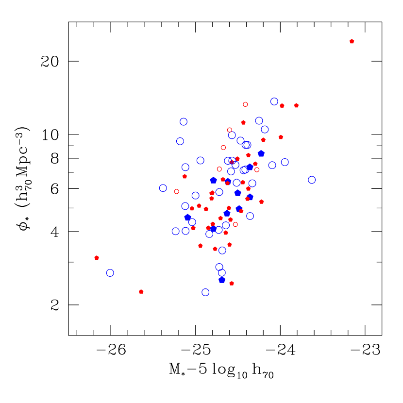
Figure A2: The LF parameters for individual clusters. Filled pentagons: clusters with $kT_{X}>3.8$ keV, open circles: those with $kT_{X}\leq 3.8$ keV. Larger symbols: clusters at $z\leq 0.043$, smaller symbols: those at $z>0.043$.

Because 2MASS is a flux-limited survey, only the brightest galaxies can be observed in more distant clusters. Therefore deriving the LF for these distant– approaching $z\sim 0.1$– clusters (especially when they are not massive) requires some extrapolation. We have examined the scaling relations by excluding those clusters whose estimated total light is more than 3 times the total observed light. The changes in the slopes of the scaling relations are within the statistical uncertainties. Finally, we consider a subsample of 49 clusters that are within HIFLUGCS (Reiprich & Böhringer 2002), which is a X–ray flux-limited sample. The scaling relations based on this subsample show slight increases in slope, but all within $1\sigma$ from those listed in Table 1.

Table 2: Derived Quantities of the Clusters

		$T_{X}$		$\phi_{*,500}$	$M_{*}-5\log h_{70}$	$L_{500}$		$L_{200}$
Name	$z$	(keV)	$N_{obs}$	($h_{70}^{3}\,$Mpc-3)	(mag)	($h_{70}^{-2}\,10^{12}L_{\odot}$)	$N_{500}$	($h_{70}^{-2}\,10^{12}L_{\odot}$)	$N_{200}$
(1)	(2)	(3)	(4)	(5)	(6)	(7)	(8)	(9)	(10)
a2319	0.0557	$11.8^{0.09}_{0.09}$	74	$4.54\pm 0.41$	$-24.70\pm 0.23$	$14.63\pm 0.04$	$267\pm 32$	$22.17\pm 0.03$	$399\pm 46$
trian	0.0510	$9.5^{0.42}_{0.42}$	62	$4.14\pm 0.43$	$-24.85\pm 0.26$	$12.01\pm 0.05$	$184\pm 25$	$18.01\pm 0.04$	$283\pm 35$
a2029	0.0773	$8.7^{0.18}_{0.18}$	14	$5.30\pm 1.38$	$-24.22\pm 0.55$	$8.12\pm 0.06$	$155\pm 44$	$13.14\pm 0.05$	$277\pm 76$
a2142	0.0899	$8.68^{0.12}_{0.12}$	12	$3.96\pm 1.01$	$-24.64\pm 0.58$	$7.20\pm 0.09$	$134\pm 38$	$13.38\pm 0.06$	$265\pm 70$
a0754	0.0542	$8.5^{0.3}_{0.3}$	47	$4.30\pm 0.50$	$-24.80\pm 0.30$	$9.28\pm 0.05$	$156\pm 24$	$12.79\pm 0.04$	$232\pm 35$
a1656	0.0232	$8.21^{0.16}_{0.16}$	122	$4.10\pm 0.38$	$-24.79\pm 0.26$	$8.94\pm 0.05$	$147\pm 18$	$12.58\pm 0.05$	$220\pm 25$
a2256	0.0601	$7.51^{0.11}_{0.11}$	45	$6.55\pm 0.69$	$-24.68\pm 0.29$	$10.11\pm 0.04$	$186\pm 26$	$14.27\pm 0.04$	$265\pm 38$
a3667	0.0560	$7^{0.36}_{0.36}$	41	$4.95\pm 0.60$	$-24.88\pm 0.31$	$8.65\pm 0.06$	$136\pm 22$	$12.76\pm 0.04$	$233\pm 34$
a2255	0.0806	$6.87^{1.7}_{1.1}$	21	$5.10\pm 0.74$	$-24.96\pm 0.41$	$8.70\pm 0.08$	$135\pm 26$	$12.28\pm 0.08$	$185\pm 36$
a0478	0.0881	$6.84^{0.13}_{0.13}$	11	$6.32\pm 1.36$	$-24.62\pm 0.58$	$7.96\pm 0.09$	$146\pm 35$	$12.95\pm 0.06$	$321\pm 117$
a1650	0.0845	$6.7^{0.5}_{0.5}$	5	$2.45\pm 1.21$	$-24.57\pm 1.01$	$3.09\pm 0.14$	$54\pm 29$	$6.97\pm 0.07$	$172\pm 86$
a0644	0.0704	$6.59^{0.1}_{0.1}$	19	$6.37\pm 1.08$	$-24.44\pm 0.45$	$6.34\pm 0.06$	$133\pm 28$	$9.05\pm 0.06$	$166\pm 37$
a0426	0.0183	$6.33^{0.21}_{0.18}$	120	$4.57\pm 0.44$	$-25.09\pm 0.29$	$8.63\pm 0.07$	$122\pm 15$	$12.12\pm 0.05$	$205\pm 21$
a1651	0.0860	$6.3^{0.3}_{0.3}$	10	$13.14\pm 4.28$	$-23.98\pm 0.64$	$7.82\pm 0.05$	$205\pm 63$	$12.05\pm 0.04$	$383\pm 197$
a3266	0.0594	$6.2^{0.5}_{0.4}$	32	$5.47\pm 0.72$	$-24.81\pm 0.35$	$7.79\pm 0.06$	$121\pm 21$	$11.71\pm 0.04$	$217\pm 34$
a0085	0.0551	$6.1^{0.12}_{0.12}$	27	$5.00\pm 0.76$	$-24.61\pm 0.39$	$5.99\pm 0.06$	$101\pm 20$	$8.02\pm 0.05$	$156\pm 32$
a2420	0.0846	$6^{2.3}_{1.2}$	8	$4.86\pm 1.61$	$-24.46\pm 0.75$	$4.71\pm 0.10$	$86\pm 32$	$8.40\pm 0.06$	$241\pm 140$
a0119	0.0440	$5.8^{0.36}_{0.36}$	40	$4.13\pm 0.56$	$-25.03\pm 0.34$	$6.46\pm 0.07$	$91\pm 16$	$10.10\pm 0.08$	$133\pm 21$
a3391	0.0531	$5.7^{0.42}_{0.42}$	23	$3.50\pm 0.61$	$-24.94\pm 0.44$	$5.84\pm 0.09$	$72\pm 16$	$9.29\pm 0.07$	$132\pm 25$
a3558	0.0480	$5.7^{0.12}_{0.12}$	60	$6.73\pm 0.68$	$-25.13\pm 0.26$	$11.10\pm 0.06$	$147\pm 20$	$17.98\pm 0.05$	$260\pm 28$
a3158	0.0590	$5.5^{0.3}_{0.4}$	31	$7.70\pm 0.98$	$-24.57\pm 0.35$	$6.76\pm 0.05$	$129\pm 22$	$9.13\pm 0.05$	$169\pm 30$
a1991	0.0590	$5.4^{5.9}_{2.2}$	17	$4.48\pm 0.90$	$-24.59\pm 0.50$	$4.06\pm 0.07$	$73\pm 19$	$5.47\pm 0.06$	$108\pm 32$
a2065	0.0726	$5.37^{0.206}_{0.181}$	23	$11.20\pm 1.41$	$-24.44\pm 0.38$	$7.33\pm 0.05$	$167\pm 28$	$12.40\pm 0.03$	$329\pm 60$
a1795	0.0631	$5.34^{0.07}_{0.07}$	17	$9.76\pm 1.90$	$-23.99\pm 0.48$	$4.80\pm 0.04$	$123\pm 29$	$6.25\pm 0.04$	$182\pm 58$
a3822	0.0760	$5.12^{0.26}_{0.187}$	16	$4.97\pm 0.86$	$-25.04\pm 0.48$	$5.38\pm 0.10$	$85\pm 19$	$9.36\pm 0.07$	$165\pm 34$
a2734	0.0620	$5.07^{0.36}_{0.42}$	11	$3.53\pm 0.94$	$-24.60\pm 0.64$	$3.13\pm 0.09$	$53\pm 17$	$4.11\pm 0.07$	$89\pm 36$
a3395sw	0.0510	$5^{0.3}_{0.3}$	30	$5.77\pm 0.81$	$-24.80\pm 0.37$	$5.61\pm 0.06$	$92\pm 17$	$7.98\pm 0.06$	$134\pm 24$
a0376	0.0484	$5^{2}_{1.1}$	29	$7.59\pm 1.10$	$-24.30\pm 0.37$	$4.57\pm 0.04$	$100\pm 19$	$6.49\pm 0.03$	$171\pm 33$
a1314	0.0335	$5^{4.5}_{1.8}$	22	$2.53\pm 0.64$	$-24.69\pm 0.58$	$2.48\pm 0.09$	$40\pm 13$	$2.60\pm 0.16$	$38\pm 20$
a2147	0.0351	$4.91^{0.18}_{0.18}$	42	$5.76\pm 0.80$	$-24.50\pm 0.35$	$4.15\pm 0.05$	$81\pm 15$	$7.58\pm 0.04$	$150\pm 22$
a3112	0.0750	$4.7^{0.24}_{0.24}$	8	$6.00\pm 1.73$	$-24.38\pm 0.71$	$4.11\pm 0.08$	$71\pm 24$	$6.44\pm 0.06$	$150\pm 57$
a1644	0.0474	$4.7^{0.9}_{0.7}$	34	$7.96\pm 1.03$	$-24.51\pm 0.34$	$5.82\pm 0.05$	$103\pm 18$	$7.91\pm 0.04$	$150\pm 25$
a2199	0.0303	$4.5^{0.2}_{0.1}$	52	$7.35\pm 0.93$	$-24.36\pm 0.32$	$4.43\pm 0.04$	$86\pm 15$	$6.88\pm 0.04$	$138\pm 20$
a2107	0.0421	$4.31^{0.57}_{0.35}$	23	$5.54\pm 1.03$	$-24.36\pm 0.46$	$3.26\pm 0.05$	$60\pm 15$	$4.38\pm 0.07$	$76\pm 19$
a0193	0.0486	$4.2^{1}_{0.5}$	17	$5.45\pm 1.13$	$-24.39\pm 0.52$	$3.16\pm 0.06$	$57\pm 15$	$4.05\pm 0.05$	$83\pm 24$
a2063	0.0355	$4.1^{0.6}_{0.6}$	38	$8.36\pm 1.16$	$-24.23\pm 0.35$	$3.50\pm 0.04$	$79\pm 15$	$4.53\pm 0.04$	$107\pm 21$
a4059	0.0475	$4.1^{0.18}_{0.18}$	14	$3.40\pm 0.83$	$-24.77\pm 0.60$	$3.12\pm 0.10$	$39\pm 12$	$4.71\pm 0.07$	$78\pm 20$
a1767	0.0701	$4.1^{1.8}_{0.9}$	11	$8.23\pm 1.77$	$-24.38\pm 0.58$	$4.20\pm 0.07$	$79\pm 21$	$5.36\pm 0.07$	$99\pm 31$
a0576	0.0389	$4.02^{0.07}_{0.07}$	35	$6.49\pm 0.92$	$-24.79\pm 0.36$	$4.62\pm 0.06$	$74\pm 14$	$7.55\pm 0.04$	$143\pm 21$
a3376	0.0456	$4^{0.4}_{0.4}$	27	$9.51\pm 1.41$	$-24.20\pm 0.39$	$3.81\pm 0.04$	$85\pm 17$	$5.02\pm 0.04$	$117\pm 25$

Table 2: Derived Quantities of the Clusters (Continued)

		$T_{X}$		$\phi_{*,500}$	$M_{*}-5\log h_{70}$	$L_{500}$		$L_{200}$
Name	$z$	(keV)	$N_{obs}$	($h_{70}^{3}\,$Mpc-3)	(mag)	($h_{70}^{-2}\,10^{12}L_{\odot}$)	$N_{500}$	($h_{70}^{-2}\,10^{12}L_{\odot}$)	$N_{200}$
(1)	(2)	(3)	(4)	(5)	(6)	(7)	(8)	(9)	(10)
a0133	0.0569	$3.97^{0.17}_{0.17}$	15	$13.16\pm 2.63$	$-23.81\pm 0.51$	$3.72\pm 0.04$	$96\pm 24$	$5.35\pm 0.03$	$150\pm 40$
a0496	0.0328	$3.91^{0.04}_{0.04}$	37	$6.42\pm 0.94$	$-24.62\pm 0.37$	$3.91\pm 0.05$	$66\pm 13$	$5.47\pm 0.04$	$106\pm 18$
a1185	0.0325	$3.9^{2}_{1.1}$	28	$4.74\pm 0.87$	$-24.63\pm 0.45$	$2.84\pm 0.07$	$49\pm 12$	$4.13\pm 0.06$	$76\pm 17$
awm7	0.0172	$3.9^{0.12}_{0.12}$	51	$4.96\pm 0.79$	$-24.49\pm 0.48$	$2.90\pm 0.06$	$50\pm 10$	$3.62\pm 0.06$	$74\pm 15$
a2440	0.0904	$3.88^{0.16}_{0.14}$	5	$2.26\pm 0.75$	$-25.64\pm 0.88$	$3.35\pm 0.33$	$30\pm 12$	$4.51\pm 0.27$	$45\pm 19$
a3560	0.0489	$3.87^{0.22}_{0.19}$	24	$3.12\pm 0.56$	$-26.17\pm 0.44$	$6.50\pm 0.27$	$50\pm 11$	$9.52\pm 0.18$	$82\pm 15$
a0780	0.0538	$3.8^{0.12}_{0.12}$	11	$24.14\pm 7.35$	$-23.16\pm 0.61$	$3.09\pm 0.02$	$117\pm 37$	$3.24\pm 0.04$	$90\pm 35$
a3562	0.0499	$3.8^{0.5}_{0.5}$	20	$5.74\pm 1.02$	$-24.81\pm 0.45$	$3.23\pm 0.08$	$59\pm 14$	$6.40\pm 0.05$	$118\pm 22$
a2670	0.0762	$3.73^{0.17}_{0.13}$	13	$13.31\pm 2.18$	$-24.41\pm 0.51$	$5.74\pm 0.06$	$111\pm 23$	$8.72\pm 0.05$	$174\pm 36$
a2657	0.0404	$3.7^{0.3}_{0.3}$	17	$4.07\pm 0.90$	$-24.73\pm 0.55$	$2.35\pm 0.09$	$40\pm 11$	$2.84\pm 0.09$	$52\pm 16$
a1142	0.0349	$3.7^{1.7}_{1.1}$	13	$2.25\pm 0.70$	$-24.88\pm 0.77$	$1.84\pm 0.14$	$24\pm 9$	$2.71\pm 0.16$	$37\pm 14$
a2634	0.0314	$3.7^{0.18}_{0.18}$	38	$5.62\pm 0.83$	$-25.00\pm 0.38$	$4.53\pm 0.08$	$61\pm 12$	$6.62\pm 0.06$	$104\pm 17$
2a0335	0.0349	$3.64^{0.054}_{0.048}$	28	$5.81\pm 0.95$	$-24.72\pm 0.41$	$3.44\pm 0.07$	$56\pm 12$	$5.29\pm 0.07$	$86\pm 16$
a3526	0.0114	$3.54^{0.08}_{0.08}$	59	$4.02\pm 0.71$	$-25.12\pm 0.67$	$3.66\pm 0.16$	$44\pm 10$	$5.24\pm 0.18$	$68\pm 14$
a1367	0.0216	$3.5^{0.11}_{0.11}$	60	$7.81\pm 0.99$	$-24.62\pm 0.34$	$3.81\pm 0.05$	$69\pm 12$	$5.46\pm 0.06$	$93\pm 15$
mkw03s	0.0434	$3.5^{0.12}_{0.12}$	13	$4.28\pm 1.08$	$-24.53\pm 0.62$	$1.96\pm 0.08$	$36\pm 12$	$2.76\pm 0.06$	$61\pm 19$
a1736	0.0458	$3.5^{0.4}_{0.4}$	27	$5.84\pm 0.93$	$-25.22\pm 0.40$	$5.28\pm 0.10$	$62\pm 13$	$10.97\pm 0.08$	$127\pm 18$
hcg094	0.0417	$3.45^{0.3}_{0.3}$	12	$3.35\pm 0.94$	$-24.68\pm 0.69$	$2.51\pm 0.11$	$29\pm 10$	$4.37\pm 0.12$	$53\pm 14$
a2589	0.0416	$3.38^{0.08}_{0.08}$	18	$6.31\pm 1.32$	$-24.33\pm 0.52$	$2.51\pm 0.06$	$46\pm 13$	$2.91\pm 0.05$	$65\pm 20$
mkw08	0.0270	$3.29^{0.23}_{0.22}$	24	$4.25\pm 0.91$	$-24.64\pm 0.56$	$2.13\pm 0.08$	$34\pm 9$	$2.69\pm 0.09$	$46\pm 13$
a4038	0.0283	$3.15^{0.06}_{0.06}$	34	$7.07\pm 1.13$	$-24.58\pm 0.41$	$2.85\pm 0.06$	$52\pm 11$	$3.55\pm 0.06$	$70\pm 15$
a1060	0.0114	$3.1^{0.15}_{0.15}$	69	$7.18\pm 1.07$	$-24.41\pm 0.52$	$2.39\pm 0.06$	$49\pm 10$	$3.17\pm 0.08$	$68\pm 14$
a2052	0.0348	$3.1^{0.2}_{0.2}$	30	$9.07\pm 1.39$	$-24.41\pm 0.39$	$3.22\pm 0.05$	$60\pm 12$	$4.43\pm 0.04$	$93\pm 18$
a0548e	0.0395	$3.1^{0.1}_{0.1}$	30	$7.83\pm 1.18$	$-24.94\pm 0.38$	$4.17\pm 0.08$	$63\pm 12$	$6.70\pm 0.06$	$107\pm 17$
a2593	0.0433	$3.1^{1.5}_{0.9}$	22	$7.22\pm 1.27$	$-24.72\pm 0.45$	$3.38\pm 0.07$	$53\pm 12$	$5.41\pm 0.06$	$90\pm 17$
a0539	0.0288	$3.04^{0.066}_{0.06}$	44	$9.95\pm 1.31$	$-24.57\pm 0.33$	$3.72\pm 0.05$	$68\pm 12$	$4.98\pm 0.04$	$101\pm 16$
as1101	0.0580	$3^{1.2}_{0.7}$	8	$7.18\pm 2.01$	$-24.28\pm 0.72$	$2.18\pm 0.08$	$41\pm 15$	$3.16\pm 0.05$	$75\pm 27$
a0779	0.0230	$2.97^{0.24}_{0.24}$	15	$2.71\pm 0.85$	$-24.69\pm 0.88$	$1.72\pm 0.14$	$19\pm 8$	$2.25\pm 0.19$	$27\pm 11$
awm4	0.0326	$2.92^{0.24}_{0.24}$	12	$6.52\pm 2.03$	$-23.63\pm 0.71$	$1.48\pm 0.04$	$28\pm 11$	$1.73\pm 0.04$	$39\pm 18$
exo0422	0.0390	$2.9^{0.5}_{0.4}$	11	$4.63\pm 1.35$	$-24.36\pm 0.71$	$1.63\pm 0.08$	$27\pm 10$	$2.04\pm 0.06$	$42\pm 16$
a2626	0.0553	$2.9^{2.5}_{1}$	15	$8.85\pm 1.61$	$-24.67\pm 0.50$	$3.57\pm 0.08$	$57\pm 14$	$4.49\pm 0.07$	$77\pm 20$
zw1615	0.0302	$2.9^{2.6}_{1.1}$	23	$7.49\pm 1.58$	$-24.09\pm 0.50$	$1.68\pm 0.05$	$40\pm 11$	$2.18\pm 0.05$	$53\pm 17$
mkw09	0.0397	$2.66^{0.57}_{0.57}$	12	$7.71\pm 2.08$	$-23.95\pm 0.65$	$1.48\pm 0.05$	$33\pm 12$	$2.27\pm 0.05$	$54\pm 17$
a0194	0.0180	$2.63^{0.15}_{0.15}$	24	$3.91\pm 0.97$	$-24.84\pm 0.73$	$1.97\pm 0.13$	$24\pm 8$	$2.85\pm 0.31$	$29\pm 10$
a0168	0.0450	$2.6^{1.1}_{0.6}$	21	$10.45\pm 1.74$	$-24.60\pm 0.44$	$3.17\pm 0.06$	$55\pm 13$	$4.25\pm 0.05$	$84\pm 18$
a0400	0.0240	$2.43^{0.078}_{0.072}$	29	$7.82\pm 1.40$	$-24.57\pm 0.46$	$2.34\pm 0.06$	$38\pm 9$	$3.46\pm 0.05$	$65\pm 13$
a0262	0.0161	$2.41^{0.03}_{0.03}$	39	$7.52\pm 1.33$	$-24.53\pm 0.51$	$2.07\pm 0.07$	$36\pm 8$	$3.03\pm 0.06$	$60\pm 12$
a2151	0.0369	$2.4^{0.06}_{0.06}$	21	$6.04\pm 1.18$	$-25.38\pm 0.48$	$3.44\pm 0.14$	$38\pm 9$	$5.17\pm 0.09$	$70\pm 13$
mkw04s	0.0283	$2.13^{0.4}_{0.4}$	8	$2.86\pm 1.21$	$-24.72\pm 1.08$	$1.36\pm 0.17$	$12\pm 6$	$1.59\pm 0.10$	$22\pm 10$
a3389	0.0265	$2.1^{0.9}_{0.6}$	25	$7.35\pm 1.42$	$-25.12\pm 0.48$	$2.81\pm 0.11$	$35\pm 8$	$4.09\pm 0.08$	$61\pm 12$
ivzw038	0.0170	$2.07^{0.56}_{0.42}$	20	$4.37\pm 1.20$	$-25.04\pm 0.79$	$1.76\pm 0.17$	$20\pm 7$	$2.34\pm 0.12$	$35\pm 10$
as0636	0.0116	$2.06^{0.07}_{0.06}$	31	$5.09\pm 1.23$	$-25.12\pm 0.83$	$1.89\pm 0.19$	$24\pm 7$	$2.40\pm 0.24$	$32\pm 10$
a3581	0.0230	$1.83^{0.04}_{0.04}$	15	$6.34\pm 1.71$	$-24.51\pm 0.70$	$1.22\pm 0.09$	$20\pm 7$	$1.52\pm 0.16$	$22\pm 8$
mkw04	0.0200	$1.71^{0.09}_{0.09}$	13	$4.01\pm 1.32$	$-25.23\pm 0.90$	$1.71\pm 0.23$	$15\pm 6$	$2.35\pm 0.26$	$22\pm 8$
ngc6338	0.0282	$1.69^{0.16}_{0.16}$	15	$9.07\pm 2.22$	$-24.39\pm 0.61$	$1.58\pm 0.07$	$23\pm 7$	$1.69\pm 0.07$	$29\pm 10$
a0076	0.0405	$1.5^{1.1}_{0.6}$	15	$11.29\pm 2.42$	$-25.14\pm 0.53$	$2.03\pm 0.13$	$30\pm 8$	$3.56\pm 0.06$	$58\pm 13$
ngc6329	0.0276	$1.45^{0.08}_{0.08}$	13	$9.46\pm 2.49$	$-24.47\pm 0.66$	$1.26\pm 0.08$	$20\pm 7$	$1.56\pm 0.09$	$26\pm 9$
as0805	0.0140	$1.4^{0.3}_{0.3}$	28	$13.67\pm 2.85$	$-24.07\pm 0.57$	$1.30\pm 0.05$	$23\pm 6$	$1.75\pm 0.09$	$30\pm 9$
ngc0507	0.0165	$1.26^{0.07}_{0.07}$	21	$9.39\pm 2.23$	$-25.18\pm 0.63$	$1.94\pm 0.16$	$21\pm 6$	$2.57\pm 0.18$	$28\pm 8$
ngc2563	0.0163	$1.06^{0.04}_{0.04}$	13	$10.50\pm 3.33$	$-24.18\pm 0.85$	$0.75\pm 0.08$	$12\pm 5$	$1.08\pm 0.08$	$21\pm 7$
wp23	0.0087	$1^{0.6}_{0.4}$	7	$2.71\pm 2.71$	$-26.01\pm 2.83$	$0.89\pm 0.89$	$6\pm 6$	$1.09\pm 0.93$	$10\pm 10$
ic4296	0.0133	$0.95^{0.09}_{0.09}$	14	$11.41\pm 3.66$	$-24.25\pm 0.90$	$1.25\pm 0.09$	$12\pm 5$	$1.63\pm 0.13$	$18\pm 7$
hcg062	0.0137	$0.87^{0.02}_{0.02}$	8	$7.15\pm 3.42$	$-24.43\pm 1.37$	$0.59\pm 0.17$	$7\pm 4$	$0.92\pm 0.23$	$12\pm 6$

References

- Abadi et al. (1999) Abadi, M. G., Moore, B., & Bower, R. G. 1999, MNRAS, 308, 947
- Adami et al. (1998) Adami, C., Mazure, A., Katgert, P., & Biviano, A. 1998, A&A, 336, 63
- Adami et al. (2001) Adami, C., Mazure, A., Ulmer, M. P., & Savine, C. 2001, A&A, 371, 11
- Andreon (2001) Andreon, S. 2001, ApJ, 547, 623
- Andreon (2003) —. 2003, A&A, accepted, astro-ph/0312120
- Andreon & Pelló (2000) Andreon, S. & Pelló, R. 2000, A&A, 353, 479
- Arabadjis et al. (2002) Arabadjis, J. S., Bautz, M. W., & Garmire, G. P. 2002, ApJ, 572, 66
- Böhringer et al. (2000) Böhringer, H., Voges, W., Huchra, J. P., McLean, B., Giacconi, R., Rosati, P., Burg, R., Mader, J., Schuecker, P., Simiç, D., Komossa, S., Reiprich, T. H., Retzlaff, J., & Trümper, J. 2000, ApJS, 129, 435
- Bahcall & Comerford (2002) Bahcall, N. A. & Comerford, J. M. 2002, ApJ, 565, L5
- Balogh et al. (2001) Balogh, M. L., Christlein, D., Zabludoff, A. I., & Zaritsky, D. 2001, ApJ, 557, 117
- Bartelmann (1996) Bartelmann, M. 1996, A&A, 313, 697
- Bell et al. (2003) Bell, E. F., McIntosh, D. H., Katz, N., & Weinberg, M. D. 2003, ApJS, 149, 289
- Bennett et al. (2003) Bennett, C. L., Halpern, M., Hinshaw, G., Jarosik, N., Kogut, A., Limon, M., Meyer, S. S., Page, L., Spergel, D. N., Tucker, G. S., Wollack, E., Wright, E. L., Barnes, C., Greason, M. R., Hill, R. S., Komatsu, E., Nolta, M. R., Odegard, N., Peiris, H. V., Verde, L., & Weiland, J. L. 2003, ApJS, 148, 1
- Benson et al. (2003) Benson, A. J., Bower, R. G., Frenk, C. S., Lacey, C. G., Baugh, C. M., & Cole, S. 2003, ApJ, 599, 38
- Benson et al. (2000) Benson, A. J., Cole, S., Frenk, C. S., Baugh, C. M., & Lacey, C. G. 2000, MNRAS, 311, 793
- Berlind & Weinberg (2002) Berlind, A. A. & Weinberg, D. H. 2002, ApJ, 575, 587
- Berlind et al. (2003) Berlind, A. A., Weinberg, D. H., Benson, A. J., Baugh, C. M., Cole, S., Davé, R., Frenk, C. S., Jenkins, A., Katz, N., & Lacey, C. G. 2003, ApJ, 593, 1
- Biviano & Girardi (2003) Biviano, A. & Girardi, M. 2003, ApJ, 585, 205
- Blake & Wall (2002) Blake, C. & Wall, J. 2002, MNRAS, 337, 993
- Bullock et al. (2001) Bullock, J. S., Kolatt, T. S., Sigad, Y., Somerville, R. S., Kravtsov, A. V., Klypin, A. A., Primack, J. R., & Dekel, A. 2001, MNRAS, 321, 559
- Carlberg et al. (1997) Carlberg, R. G., Yee, H. K. C., Ellingson, E., Morris, S. L., Abraham, R., Gravel, P., Pritchet, C. J., Smecker-Hane, T., Hartwick, F. D. A., Hesser, J. E., Hutchings, J. B., & Oke, J. B. 1997, ApJ, 485, L13
- Christlein & Zabludoff (2003) Christlein, D. & Zabludoff, A. I. 2003, ApJ, 591, 764
- Clowe & Schneider (2002) Clowe, D. & Schneider, P. 2002, A&A, 395, 385
- Cole et al. (2000) Cole, S., Lacey, C. G., Baugh, C. M., & Frenk, C. S. 2000, MNRAS, 319, 168
- David et al. (1993) David, L. P., Slyz, A., Jones, C., Forman, W., Vrtilek, S. D., & Arnaud, K. A. 1993, ApJ, 412, 479
- De Lucia et al. (2004) De Lucia, G., Kauffmann, G., Springel, V., White, S. D. M., Lanzoni, B., Stoehr, F., Tormen, G., & Yoshida, N. 2004, MNRAS, 348, 333
- De Propris et al. (2003) De Propris, R., Colless, M., Driver, S. P., Couch, W., Peacock, J. A., Baldry, I. K., Baugh, C. M., Bland-Hawthorn, J., Bridges, T., Cannon, R., Cole, S., Collins, C., Cross, N., Dalton, G. B., Efstathiou, G., Ellis, R. S., Frenk, C. S., Glazebrook, K., Hawkins, E., Jackson, C., Lahav, O., Lewis, I., Lumsden, S., Maddox, S., Madgwick, D. S., Norberg, P., Percival, W., Peterson, B., Sutherland, W., & Taylor, K. 2003, MNRAS, 342, 725
- De Propris et al. (1998) De Propris, R., Eisenhardt, P. R., Stanford, S. A., & Dickinson, M. 1998, ApJ, 503, L45
- De Propris et al. (1999) De Propris, R., Stanford, S. A., Eisenhardt, P. R., Dickinson, M., & Elston, R. 1999, AJ, 118, 719
- Diemand et al. (2004) Diemand, J., Moore, B., & Stadel, J. 2004, MNRAS, submitted, astro-ph/0402160
- Ebeling et al. (1998) Ebeling, H., Edge, A. C., Bohringer, H., Allen, S. W., Crawford, C. S., Fabian, A. C., Voges, W., & Huchra, J. P. 1998, MNRAS, 301, 881
- Ebeling et al. (1996) Ebeling, H., Voges, W., Bohringer, H., Edge, A. C., Huchra, J. P., & Briel, U. G. 1996, MNRAS, 281, 799
- Evrard et al. (1996) Evrard, A. E., Metzler, C. A., & Navarro, J. F. 1996, ApJ, 469, 494
- Feulner et al. (2003) Feulner, G., Bender, R., Drory, N., Hopp, U., Snigula, J., & Hill, G. J. 2003, MNRAS, 342, 605
- Finoguenov et al. (2001) Finoguenov, A., Reiprich, T. H., & Böhringer, H. 2001, A&A, 368, 749
- Geller et al. (1999) Geller, M. J., Diaferio, A., & Kurtz, M. J. 1999, ApJ, 517, L23
- Girardi et al. (2002) Girardi, M., Manzato, P., Mezzetti, M., Giuricin, G., & Limboz, F. 2002, ApJ, 569, 720
- Gnedin (2003) Gnedin, O. Y. 2003, ApJ, 589, 752
- Gonzalez et al. (2000) Gonzalez, A. H., Zabludoff, A. I., Zaritsky, D., & Dalcanton, J. J. 2000, ApJ, 536, 561
- Goto et al. (2002) Goto, T., Okamura, S., McKay, T. A., Bahcall, N. A., Annis, J., Bernard, M., Brinkmann, J., Gómez, P. L., Hansen, S., Kim, R. S. J., Sekiguchi, M., & Sheth, R. K. 2002, PASJ, 54, 515
- Hayashi et al. (2003) Hayashi, E., Navarro, J. F., Taylor, J. E., Stadel, J., & Quinn, T. 2003, ApJ, 584, 541
- Hu (2003) Hu, W. 2003, Phys. Rev. D, 67, 81304
- Jarrett et al. (2000) Jarrett, T. H., Chester, T., Cutri, R., Schneider, S., Skrutskie, M., & Huchra, J. P. 2000, AJ, 119, 2498
- Jenkins et al. (2001) Jenkins, A., Frenk, C. S., White, S. D. M., Colberg, J. M., Cole, S., Evrard, A. E., Couchman, H. M. P., & Yoshida, N. 2001, MNRAS, 321, 372
- Katgert et al. (2004) Katgert, P., Biviano, A., & Mazure, A. 2004, ApJ, 600, 657
- Kauffmann et al. (1999) Kauffmann, G., Colberg, J. M., Diaferio, A., & White, S. D. M. 1999, MNRAS, 303, 188
- Kauffmann et al. (1993) Kauffmann, G., White, S. D. M., & Guiderdoni, B. 1993, MNRAS, 264, 201
- Klypin et al. (1999) Klypin, A., Gottlöber, S., Kravtsov, A. V., & Khokhlov, A. M. 1999, ApJ, 516, 530
- Kochanek et al. (2001) Kochanek, C. S., Pahre, M. A., Falco, E. E., Huchra, J. P., Mader, J., Jarrett, T. H., Chester, T., Cutri, R., & Schneider, S. E. 2001, ApJ, 560, 566
- Kochanek et al. (2003) Kochanek, C. S., White, M., Huchra, J., Macri, L., Jarrett, T. H., Schneider, S. E., & Mader, J. 2003, ApJ, 585, 161
- Kravtsov et al. (2003) Kravtsov, A. V., Berlind, A. A., Wechsler, R. H., Klypin, A. A., Gottloeber, S., Allgood, B., & Primack, J. R. 2003, ApJ, submitted, astro-ph/0308519
- Lewis et al. (2003) Lewis, A. D., Buote, D. A., & Stocke, J. T. 2003, ApJ, 586, 135
- Lin et al. (2003) Lin, Y.-T., Mohr, J. J., & Stanford, S. A. 2003, ApJ, 591, 749
- Madau et al. (1998) Madau, P., Pozzetti, L., & Dickinson, M. 1998, ApJ, 498, 106
- Magliocchetti & Porciani (2003) Magliocchetti, M. & Porciani, C. 2003, MNRAS, 346, 186
- Majumdar & Mohr (2003) Majumdar, S. & Mohr, J. J. 2003, ApJ, submitted, astro-ph/0305341
- Maller et al. (2003) Maller, A. H., McIntosh, D. H., Katz, N., & Weinberg, M. D. 2003, ApJ, submitted (astro-ph/0304005)
- Malumuth & Richstone (1984) Malumuth, E. M. & Richstone, D. O. 1984, ApJ, 276, 413
- Marinoni & Hudson (2002) Marinoni, C. & Hudson, M. J. 2002, ApJ, 569, 101
- Merritt (1984) Merritt, D. 1984, ApJ, 276, 26
- Mo & White (1996) Mo, H. J. & White, S. D. M. 1996, MNRAS, 282, 347
- Mohr et al. (1999) Mohr, J. J., Mathiesen, B., & Evrard, A. E. 1999, ApJ, 517, 627
- Mohr et al. (2000) Mohr, J. J., Reese, E. D., Ellingson, E., Lewis, A. D., & Evrard, A. E. 2000, ApJ, 544, 109
- Moore et al. (1998) Moore, B., Governato, F., Quinn, T., Stadel, J., & Lake, G. 1998, ApJ, 499, L5
- Navarro et al. (1997) Navarro, J. F., Frenk, C. S., & White, S. D. M. 1997, ApJ, 490, 493
- Navarro et al. (2003) Navarro, J. F., Hayashi, E., Power, C., Jenkins, A., Frenk, C. S., White, S. D. M., Springel, V., Stadel, J., & Quinn, T. R. 2003, MNRAS, submitted, astro-ph/0311231
- Oemler (1976) Oemler, A. 1976, ApJ, 209, 693
- O’Hara et al. (2003) O’Hara, T. B., Mohr, J. J., & Guerrero, M. A. 2003, ApJ, accepted, astro-ph/0311402
- Ostriker et al. (2003) Ostriker, J. P., Nagamine, K., Cen, R., & Fukugita, M. 2003, ApJ, 597, 1
- Peacock & Smith (2000) Peacock, J. A. & Smith, R. E. 2000, MNRAS, 318, 1144
- Peebles (1980) Peebles, P. 1980, The Large Scale Structure of the Universe (Princeton: Princeton University Press)
- Pisani et al. (2003) Pisani, A., Ramella, M., & Geller, M. J. 2003, AJ, 126, 1677
- Poggianti et al. (1999) Poggianti, B. M., Smail, I., Dressler, A., Couch, W. J., Barger, A. J., Butcher, H., Ellis, R. S., & Oemler, A. J. 1999, ApJ, 518, 576
- Pratt & Arnaud (2002) Pratt, G. W. & Arnaud, M. 2002, A&A, 394, 375
- Press & Schechter (1974) Press, W. H. & Schechter, P. 1974, ApJ, 187, 425
- Reiprich & Böhringer (2002) Reiprich, T. H. & Böhringer, H. 2002, ApJ, 567, 716
- Rines et al. (2003) Rines, K., Geller, M. J., Kurtz, M. J., & Diaferio, A. 2003, AJ, 126, 2152
- Rines et al. (2001) Rines, K., Geller, M. J., Kurtz, M. J., Diaferio, A., Jarrett, T. H., & Huchra, J. P. 2001, ApJ, 561, L41
- Sanderson et al. (2003) Sanderson, A. J. R., Ponman, T. J., Finoguenov, A., Lloyd-Davies, E. J., & Markevitch, M. 2003, MNRAS, 340, 989
- Schechter (1976) Schechter, P. 1976, ApJ, 203, 297
- Scoccimarro et al. (2001) Scoccimarro, R., Sheth, R. K., Hui, L., & Jain, B. 2001, ApJ, 546, 20
- Seljak (2000) Seljak, U. 2000, MNRAS, 318, 203
- Sheth & Tormen (1999) Sheth, R. K. & Tormen, G. 1999, MNRAS, 308, 119
- Springel & Hernquist (2003) Springel, V. & Hernquist, L. 2003, MNRAS, 339, 312
- Springel et al. (2001) Springel, V., White, S. D. M., Tormen, G., & Kauffmann, G. 2001, MNRAS, 328, 726
- Stanford et al. (1998) Stanford, S. A., Eisenhardt, P. R., & Dickinson, M. 1998, ApJ, 492, 461
- Trentham & Mobasher (1998) Trentham, N. & Mobasher, B. 1998, MNRAS, 299, 488
- Treu et al. (2003) Treu, T., Ellis, R. S., Kneib, J., Dressler, A., Smail, I., Czoske, O., Oemler, A., & Natarajan, P. 2003, ApJ, 591, 53
- Tully (2003) Tully, R. B. 2003, ApJ, submitted, astro-ph/0312441
- Tustin et al. (2001) Tustin, A. W., Geller, M. J., Kenyon, S. J., & Diaferio, A. 2001, AJ, 122, 1289
- van der Marel et al. (2000) van der Marel, R. P., Magorrian, J., Carlberg, R. G., Yee, H. K. C., & Ellingson, E. 2000, AJ, 119, 2038
- van Dokkum et al. (2000) van Dokkum, P. G., Franx, M., Fabricant, D., Illingworth, G. D., & Kelson, D. D. 2000, ApJ, 541, 95
- White & Rees (1978) White, S. D. M. & Rees, M. J. 1978, MNRAS, 183, 341
- Yang et al. (2003) Yang, X., Mo, H. J., & van den Bosch, F. C. 2003, MNRAS, 339, 1057
- Zehavi et al. (2003) Zehavi, I., Weinberg, D. H., Zheng, Z., Berlind, A. A., Frieman, J. A., Scoccimarro, R., Sheth, R. K., Blanton, M. R., Tegmark, M., & Mo, H. J. 2003, ApJ, submitted, astro-ph/0301280