Constraining Warm Inflation with the Cosmic Microwave Background

Abstract

We discuss the spectrum of scalar density perturbations from warm inflation when the friction coefficient $\Gamma$ in the inflaton equation is dependent on the inflaton field. The spectral index of scalar fluctuations depends on a new slow-roll parameter constructed from $\Gamma$. A numerical integration of the perturbation equations is performed for a model of warm inflation and gives a good fit to the WMAP data for reasonable values of the model’s parameters.

The inflationary paradigm has proved to be the most successful idea for providing the seeds of large scale structure in the universe. A plethora of variants of the inflationary model exist today and in most of these models, radiation is red-shifted during the expansion, resulting in a vacuum-dominated Universe, giving the name supercooled inflation. A subsequent reheating period is invoked to end inflation and fill the universe with radiation Guth (1981); Linde (1982); Albrecht and Steinhart (1982); Hawking and Moss (1982). In an alternative picture, termed warm inflation, dissipative effects, arising from inflaton interactions, are important during the inflation period, so that radiation production occurs concurrently with inflationary expansion Moss (1985); Yokoyama and Maeda (1988); Berera and Fang (1995); Berera (1995, 1996, 1997).

In this letter we shall demonstrate how it is possible to constrain a particular type of warm inflationary model using Cosmic Microwave Background observations. The model which we consider is based on broken supersymmetry and has the property that the inflaton has a two stage decay chain $\phi\to\chi\to\psi$ Berera and Ramos (2003a, b). This two stage decay occurs for a wide range of inflationary models and provides a robust realisation of warm inflation. In these models the friction coefficient $\Gamma$ in the inflaton equation is a function of the inflaton field and this feature leads to some new effects on the perturbation spectrum, which we describe here.

The development of cosmological perturbations in warm inflation has been investigated previously by several authors. Taylor and Berera Taylor and Berera (2000) have analysed the perturbation spectra by identifying the small scale thermal fluctuations with cosmological perturbations when the fluctuations cross the horizon. This technique is good for order of magnitude estimates. For a more accurate treatment of the density perturbations it is necessary to use the cosmological perturbation equations, which can be found in Lee and Fang (1999); de Oliveira and Joras (2001); chan Hwang and Noh (2002). A numerical code has recently been developed which can solve the perturbation equations for any form of friction coefficient Hall et al. (2003).

We shall consider the case where the radiation produced by the inflaton field consists of low mass particles $\psi$ which are approximately thermalised. In this case the density fluctuations arise from thermal, rather than vacuum, fluctuations Moss (1985); Berera and Fang (1995); Berera (1995, 1996, 2000); Hall et al. (2003). The intermediate particle $\chi$ is not in a thermal state and thermal corrections to the inflaton potential are suppressed. This allows us to use the zero-temperature potential during inflation. The effects of thermal corrections will be discussed in future work.

Assuming the early universe to be in homogeneous expansion with expansion rate $H(t)$, the evolution of the inflaton field $\phi$ is described by the equation

$$\ddot{\phi}+(3H+\Gamma)\dot{\phi}+V_{,\phi}=0$$ (1)

where $\Gamma(\phi)$ is the damping term and $V(\phi)$ is the inflaton potentialHosoya and aki Sakagami (1984); Moss (1985); Berera (1995). The relative strength of the thermal damping compared to the expansion damping can be expressed by a parameter $r$,

$$r={\Gamma\over 3H}$$ (2)

The strong dissipation form of warm inflation occurs for large values of $r$, as opposed to supercooled inflation in which $r$ can be neglected.

The dissipation of the inflaton’s motion is associated with the production of entropy. Energy-momentum conservation implies that

$$T(\dot{s}+3Hs)=\Gamma\dot{\phi}^{2}.$$ (3)

where $s$ is the entropy density. For the situation under discussion, the entropy density is related to the energy density in the radiation $\rho_{r}$ by $\rho_{r}=\frac{3}{4}Ts$, where $T$ is the temperature, $s=\frac{\pi^{2}}{30}g_{*}T^{3}$ and $g_{*}$ is the effective number of degrees of freedom in the radiation. In more general situations, using the entropy density is preferable to using the radiation energy density Hall et al. (2003).

The zero curvature Friedman equation completes the set of differential equations for $\phi$, $T$ and the scale factor $a$,

$$3H^{2}=8\pi G({\textstyle\frac{1}{2}}\dot{\phi}^{2}+V+{\textstyle\frac{3}{4}}Ts).$$ (4)

The slow-roll approximation consists of neglecting terms in the preceding equations with the highest order in time derivatives,

$$\dot{\phi} = {-V_{,\phi}\over 3H(1+r)}$$ (5)

$$Ts = r\dot{\phi}^{2}$$ (6)

$$3H^{2} = 8\pi GV.$$ (7)

Slow-roll automatically implies inflation, $\ddot{a}>0$.

The consistency of the slow-roll approximation is governed by a set of slow-roll parameters. Warm inflation has extra slow-roll parameters in addition to the usual set for supercooled inflation due to the presence of the damping term $\Gamma$. The ‘leading order’ slow-roll parameters are,

$$\epsilon={1\over 16\pi G}\left({V_{,\phi}\over V}\right)^{2},\quad\eta={1\over 8\pi G}\left({V_{,\phi\phi}\over V}\right),\quad\beta={1\over 8\pi G}\left({\Gamma_{,\phi}V_{,\phi}\over\Gamma V}\right)$$ (8)

The first two parameters are the standard ones introduced for supercooled inflation Liddle et al. (1994); Stewart (2002); Habib et al. (2002); Martin and Schwarz (2003). A new parameter is required when there is $\phi$ dependence in the damping term. A further slow-roll parameter is required when the potential has thermal corrections Hall et al. (2003). The slow-roll approximation is valid when all of these parameters are smaller than $1+r$. In supercooled inflation, the condition is tighter and the slow roll parameters have to be smaller than 1.

In the warm inflationary regime where $r\gg 1$, the rate of change of various slowly varying parameters are given by differentiating equations (5-7),

$${1\over H}{d\ln H\over dt} = -{1\over r}\epsilon$$ (9)

$${1\over H}{d\ln\dot{\phi}\over dt} = -{1\over r}(\eta-\beta)$$ (10)

$${1\over H}{d\ln Ts\over dt} = -{1\over r}(2\eta-\beta-\epsilon)$$ (11)

Inflation ends at the time when $\epsilon=r$, since then $\ddot{a}=\dot{H}+H^{2}=0$.

Cosmological perturbations are best described in terms of gauge invariant quantities, the curvature perturbation ${\cal R}$ Lukash (1980), and the entropy perturbation $e$ Kodama and Sasaki (1984). An analytic approximation to the density perturbation amplitude for wave number $k$ can be obtained by matching the classical perturbations to the thermal fluctuation amplitude at the crossing time $k=aH$,

$${\cal P}_{\cal R}\sim\left({\pi\over 4}\right)^{1/2}{H^{5/2}\Gamma^{1/2}T\over\dot{\phi}^{2}}.$$ (12)

This result is analogous to the result ${\cal P}_{\cal R}=H^{4}/\dot{\phi}^{2}$ for supercooled inflation.

The spectral index $n_{s}$ is defined by

$$n_{s}-1={\partial\ln{\cal P}_{\cal R}\over\partial\ln k}.$$ (13)

The slow-roll equations (9-11) enable us to express the spectral index for the amplitude (12) in terms of slow-roll parameters,

$$n_{s}-1={1\over r}\left(-{9\over 4}\epsilon+{3\over 2}\eta-{9\over 4}\beta\right).$$ (14)

The first two terms agree with reference Berera (2000). The $\beta$ term shows the dependence of the spectrum on the gradient of the damping term. For comparison, the spectral index for standard, or supercooled inflation, is $n_{s}=1-6\epsilon+2\eta$ Liddle and Lyth (1992).

There are two second-order slow-roll parameters

$$\zeta^{2}={1\over(8\pi G)^{2}}\left({V_{,\phi}V_{,\phi\phi\phi}\over V^{2}}\right),\quad\gamma={1\over 8\pi G}\left({\Gamma_{,\phi\phi}\over\Gamma}\right).$$ (15)

With these we can obtain an expression for the slope of the spectral index,

$${dn_{s}\over d\ln k}={1\over r^{2}}\left(-\frac{9}{2}\beta^{2}-\frac{27}{4}\epsilon^{2}-\frac{9}{2}\epsilon\beta+\frac{15}{4}\eta\beta+6\epsilon\eta-\frac{3}{2}\zeta^{2}+\frac{9}{2}\gamma\epsilon\right).$$ (16)

The first three terms form a negative definite combination, but other terms, including $-\zeta^{2}$, can be positive.

The effect of $\beta$ in combination with ‘new inflation’ potentials is particularly interesting. Such potentials have a maximum at $\phi=0$ and a minimum at $\phi=\phi_{0}$ Linde (1982); Albrecht and Steinhart (1982); Hawking and Moss (1982). If we take $\Gamma\propto\phi^{b}$, then the behaviour of $n_{s}$ in the vicinity of the two extrema can be determined

$$n_{s}-1\to\cases{-|\eta|(2-3b)&$\phi\to 0$\cr-\infty&$\phi\to\phi_{0}$\cr}.$$ (17)

Therefore, if $b>2/3$, there will be a value $\phi_{m}$ at which $n_{s}=1$ and $n_{s}$ is decreasing. The density perturbation amplitude has a maximum at the wave number which crossed the horizon when $\phi=\phi_{m}$, and the spectrum runs from blue to red as the wave number increases. The possibility of a spectrum which runs from blue to red is particularly interesting because it is not commonly seen in inflationary models, which typically predict red spectra. (For examples of inflation with blue spectra, see Copeland et al. (1994); Linde and Riotto (1997)).

Now consider the spectrum of density perturbations for a model with interaction Lagrangians $\frac{1}{2}g^{2}\phi^{2}\chi^{2}$ and $h\chi\bar{\psi}\psi$. The friction term can be approximated by Berera and Ramos (2003a, b)

$$\Gamma\approx{g^{3}h^{2}\phi\over 256\pi^{2}}.$$ (18)

Warm inflation occurs when $g\approx h\approx 0.1$. For coupling constants of this magnitude, quantum loop corrections to the inflaton must be suppressed by an underlying supersymmetry to prevent them violating the slow-roll conditions. The supersymmetry is broken during inflation, either spontaneously, or by soft supersymmetry breaking masses. (These soft terms are not necessarily the same soft terms which occur at the TeV scale).

We take the soft supersymmetry breaking option, with inflaton potential,

$$V(\phi)=\frac{1}{2}\mu_{0}^{2}\left(\phi^{2}\log\left({\phi^{2}\over\phi_{0}^{2}}\right)+\phi_{0}^{2}-\phi^{2}\right).$$ (19)

The damping term $\Gamma$, will be parameterised by

$$\Gamma=\Gamma_{0}{\phi\over\phi_{0}}.$$ (20)

With this combination, prolonged inflation (sixty e-folds or more)can occur for values of $\phi_{0}$ smaller than the Planck scale $m_{p}$. The running of the spectral index (16) is always negative. By contrast, in the supercooled limit $\Gamma_{0}=0$, a prolonged period of inflation requires $\phi_{0}$ to be at least $2m_{p}$ and it may not be consistent to ignore the effects of quantum gravity. The density fluctuation amplitude for supercooled inflation requires $\mu_{0}$ to be around $10^{13}$ GeV.

Our numerical code solves the homogeneous background and perturbation equations simultaneously, with no assumption of slow-roll. The reader is referred to Hall et al. (2003) for further details. The code solves for the primordial power spectrum with the input parameters $\mu_{0}$, $\phi_{0}$ and $\Gamma_{0}$ defined above. In order to compare to WMAP data, power law behaviour of the spectrum is assumed about a scale $k_{0}=0.002Mpc^{-1}$. The power spectrum is then characterised by the index, $n_{s}$ and spectral running $dn/d\ln k$.

We compute the microwave anisotropies using the CAMB code Lewis et al. (2000) and run the WMAP likelihood code Verde et al. (2003) in order to compute the likelihood fit of the model to WMAP data. Since at present we are interested in isolating the behaviour of the above warm inflationary parameters, $\mu_{0}$, $\phi_{0}$ and $\Gamma_{0}$, we assume priors for the cosmological parameters ($\Omega_{\Lambda}$, $\Omega_{b}$, $\Omega_{m}$ etc.). The assumed parameter values are given in table 1 and are taken from Bennett et al.Bennett et al. (2003). The tensor components are assumed to be negligible.

Table 1: Cosmological parameters taken from BennettBennett et al. (2003). These priors are used as inputs into the CAMB code.

Parameter	Symbol	Value
Dark energy density	$\Omega_{\Lambda}$	0.73
Baryon density	$\Omega_{b}$	0.0044
Matter density	$\Omega_{m}$	0.27
Light neutrino density	$\Omega_{\nu}$	0
Spatial curvature density	$\Omega_{k}$	0
Hubble constant	h	0.71

For given values of $\mu_{0}$ and $\Gamma_{0}$, the value of $\phi_{0}$ is chosen to normalise the amplitude of the power spectrum to the WMAP value $A_{WMAP}$ at $k=k_{0}$. (In practice, we save some computation time by fixing the value of $\phi_{0}$ and using renormalisation to rescale the model to the correct amplitude.) We have restricted the range of $\phi_{0}$ to be less than the Planck scale.

Two inflationary parameters remain to be investigated, namely $\mu_{0}$ and $\Gamma_{0}$. The $1\sigma$, $2\sigma$ and $3\sigma$ bounds for this parameter space are displayed in figure 1. Note that there is no supercooled inflationary limit ($\Gamma_{0}\rightarrow 0$) in figure 1 because the density fluctuation amplitude for supercooled inflation is too small in the parameter range shown.

The $3\sigma$ limit extends well beyond the upper edge of the figure $\Gamma_{0}>1.5\times 10^{13}GeV$. Consideration of the friction term (18) shows that a value of $\Gamma_{0}=1.5\times 10^{13}GeV$ corresponds to couplings, $g\approx h\approx 0.2$. As $g$ and $h$ increase further still ($\Gamma_{0}$ increasing), we go beyond the perturbative regime in which the potential which we are using is valid. We also expect thermal corrections to the potential to be important when the coupling constants reach this magnitude, and we shall return to this issue in future work.

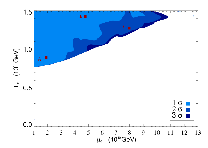
Figure 1: The $1\sigma$, $2\sigma$ and $3\sigma$ bounds on the parameters for the potential and friction term, $\mu_{0}$ and $\Gamma_{0}$ as calculated with CAMB in conjunction with the WMAP likelihood code. Values for the spectral index and spectral running at the points marked A, B and C are given in table 2.

Table 2: Spectral index and running for points A, B and C in figure 1

	$n_{s}$	$dn_{s}~{}/~{}d\ln k$
A	0.995	$-2.1\times 10^{-4}$
B	0.994	$-3.7\times 10^{-5}$
C	1.004	$-3.2\times 10^{-4}$

At points A, B and C in figure 1, the spectral index comes out very close to $n_{s}=1$ with a very small amount of spectral running (see table 2). The running of the spectrum is negative, as we predicted above, but rather small compared to some values which have been discussed in connection with the WMAP data.

Figure 2: These points represent the spectra produced for a uniformly distributed selection of parameter values $\mu_{0}$ and $\Gamma_{0}$. Note that the vertical axis is in units of $10^{-3}$.

Typical properties of the spectrum can be understood by analysing the spectra produced by a uniformly distributed set of parameter values as in figure 2. The parameter values are only included if inflation lasts long enough to affect the large scale structure. The spectra produced by these uniform parameter points are all within a small range around $n_{s}=1$ at a scale $k_{0}=0.002Mpc^{-1}$, with small spectral running. In contrast, the WMAP data can accommodate large spectral running if there are relatively large departures from $n_{s}=1$ H.V.Peiris et al. (2003), and the observations are not yet accurate enough to provide very strong restrictions on the parameter values.

We conclude by summing up the main results. For warm inflation, a third slow-roll parameter is introduced due to the dependence of the spectrum on the dissipation term, $\Gamma$. For inflation with new inflation potentials, it has been shown that, in warm inflation, one expects the spectral index to run from blue to red as the wavenumber increases. This behaviour is particularly interesting in the light of the first year WMAP data, in which such a running is hinted at. For a specific potential, representative of supersymmetry breaking, warm inflation has been compared to the WMAP data and a good fit was found for a large range of parameter values. The model produces spectra with $n_{s}$ close to one and a very small negative running of the index. Future observations of the Cosmic Microwave Background are needed to detect such small slopes in the spectrum and produce stronger constraints on the parameters.