Spectroscopic Studies of Extremely Metal-Poor Stars with Subaru/HDS:
I. Observational Data.

Abstract

We have obtained high-resolution (R $\simeq$ 50,000 or 90,000), high-quality (S/N $\gtrsim$ 100) spectra of 22 very metal-poor stars ([Fe/H] $\lesssim$ –2.5) with the High Dispersion Spectrograph fabricated for the 8.2m Subaru Telescope. The spectra cover the wavelength range from 3500 to 5100 Å; equivalent widths are measured for isolated lines of numerous elemental species, including the $\alpha$ elements, the iron-peak elements, and the light and heavy neutron-capture elements. Errors in the measurements and comparisons with previous studies are discussed. These data will be used to perform detailed abundance analyses in the following papers of this series. Radial velocities are also reported, and are compared with previous studies. At least one moderately r-process-enhanced metal-poor star, HD 186478, exhibits evidence of a small-amplitude radial velocity variation, confirming the binary status noted previously. During the course of this initial program, we have discovered a new moderately r-process-enhanced, very metal-poor star, CS 30306–132 ([Fe/H] $=-2.4$; [Eu/Fe] $=+0.85$), which is discussed in detail in the companion paper.

1 Introduction

Very metal-poor stars ([Fe/H] $\lesssim-2.5$) are believed to have been born in the early Galaxy; their chemical compositions are living records of the nucleosynthesis processes that preceded their formation. As a result of considerable efforts by many astronomers, a large list of candidate stars with [Fe/H] $<-2.5$ have been provided by wide-field objective-prism surveys in the past two decades (e.g., the HK survey: Beers et al. 1985, 1992; Beers 1999, and the Hamburg/ESO Survey: Christlieb & Beers 2000; Christlieb et al. 2001; Christlieb 2003). Over the past several years, high-resolution spectroscopic studies have enabled the measurement of elemental abundances for many of the metal-poor stars found by these surveys (e.g., McWilliam et al. 1995b; Ryan, Norris, $\&$ Beers 1996; Burris et al. 2000; Carretta et al. 2002; Cayrel et al. 2004), including detailed studies of the lowest metallicity stars yet identified (e.g., Norris, Ryan, & Beers 2001; Christlieb et al. 2002). These observational studies, which continue at present, are providing strong constraints on models of the dominant nucleosynthesis processes in the earliest epochs of star formation in our Galaxy, in particular those associated with massive stars and Type II supernovae.

Remarkable progress has been made, in particular, through studies of the neutron-capture elements in very metal-poor stars. High-resolution spectroscopic studies of very metal-poor stars have revealed, for example, that a small fraction (presently estimated to be on the order of 2%–3%, Beers, private communication) of giants with [Fe/H] $<-2.5$ exhibit large overabundances (e.g., [r-process/Fe] $>+1.0$) of neutron-capture elements associated with the r-process (e.g., [r-process/Fe] $>+1.0$ ;McWilliam et al. 1995b; Sneden et al. 2000, 2003; Cayrel et al. 2001; Hill et al. 2002). These, along with a handful of other metal-poor stars with moderately enhanced r-process elements ($+0.5\leq$ [r-process/Fe] $\leq+1.0$, e.g., Westin et al. 2000; Johnson & Bolte 2001; Cowan et al. 2002), display remarkably similar abundance patterns in the range 56 $\leq Z<$ 76, all apparently in good agreement with the solar-system r-process component. In addition, some of the neutron-capture-enhanced, metal-poor stars exhibit abundance patterns associated with s-process nucleosynthesis (e.g., Norris et al. 1997; Van Eck et al. 2001; Aoki et al. 2002; Lucatello et al. 2003).

These efforts are having a large collective impact on studies on the origin of the neutron-capture elements in the Galaxy (e.g., Ishimaru & Wanajo, 1999; Fields, Truran, & Cowan, 2002; Qian & Wasserburg, 2002), and on the underlying physics and astrophysical sites of the r- and s- processes (e.g., Gallino et al., 1998; Wanajo et al., 2002, 2003; Schatz et al., 2002; Truran et al., 2002). Furthermore, detailed studies of the r-process-enhanced, very metal-poor stars have provided new, potentially quite powerful, methods for obtaining hard lower limits on the age of the Galaxy and the universe, from the application of cosmo-chronometry based on the observed (present-day) abundance ratios of radioactive nuclei (Th and U), as compared with one another, and with stable elements originating in the r-process, (e.g., Eu, Sneden et al., 1996; Westin et al., 2000; Cayrel et al., 2001; Schatz et al., 2002; Wanajo et al., 2002, 2003; Sneden et al., 2003).

In order to develop a more clear understanding of the individual nucleosynthetic processes that were operating in the early Galaxy, further abundance studies are required, based on high-quality spectra, for much larger samples of very metal-poor stars than have been examined to date. We have initiated such a set of investigations with the Subaru Telescope High Dispersion Spectrograph (HDS, Noguchi et al. 2002). In this paper we present observations of 22 very metal-poor stars observed during the commissioning phase of this instrument. In §2 we discuss the selection of targets and details of the observations that have been carried out. Our spectra cover the wavelength range from 3500 to 5100 Å with high spectral resolution (a resolving power of $R=50,000$ or $R=90,000$) and high signal-to-noise (S/N$\gtrsim$ 100 per resolution element). We report the equivalent widths measured for the spectra in §3, where we also discuss the random errors of our measurements, and make comparisons with previous studies of stars in common. Radial velocity measurements for our program stars are presented in §4, along with a comparison with previous measurements for a number of stars. These data will be used in the detailed abundance analyses that will follow in additional papers of this series.

2 Observations

2.1 Selection of Targets

The present work is focused primarily on the observed abundance patterns of r-process elements in very metal-poor stars. Accordingly, our sample was selected to include stars that fall into one of several categories: (1) Very metal-poor stars that were previously known to exhibit extremely large enhancements of their r-process elements (CS 22892–052 and CS 31082–001: Sneden et al. 1996; Cayrel et al. 2001); (2) Bright metal-poor stars that were studied by previous authors (e.g., McWilliam et al. 1995b; Burris et al. 2000), and shown to be moderately r-process-element-rich; (3) Candidate very metal-poor giants discovered in the course of the HK survey of Beers and colleagues (Beers, Preston, & Shectman, 1992; Bonifacio, Monai, & Beers, 2000; Allende Prieto et al., 2000). For the majority of these stars, no elemental abundance results based on high-resolution spectroscopy has been previously obtained. Due to the selection criteria employed, it should be noted that our sample emphasizes stars that are either definite, or suspected, r-process-enhanced, metal-poor stars, which will impact the discussion of the distribution of the observed abundances of neutron-capture elements for these stars presented in Honda et al. (2003; Paper II).

Since our primary purpose is to investigate the neutron-capture elements, we selected giants, whose metal lines are generally stronger than metal-poor dwarfs near the main-sequence turnoff due to their lower effective temperatures. Exceptions are HD 140283 and BS 17583–100, which were observed for comparison purposes. A rather large fraction of very metal-poor stars exhibit enhancements of carbon (e.g., Beers et al. 1992, Rossi et al. 1999), up to 25% by some recent estimates. However, strongly carbon-enhanced stars ([C/Fe] $\gtrsim$ +1.0) are excluded from our sample, because contamination arising from molecular lines (CH and CN) makes the analysis of lines of neutron-capture elements difficult, and causes particular problems with regard to features of Th and U. An exception is the star CS 22892–052, which is known to exhibit an extremely large excess of r-process elements, and a large carbon enhancement, on the order of [C/Fe] $\approx+1.1$ (see Norris, Ryan, & Beers 1997 for a discussion of the impact on studies of Th in such stars).

The 22 stars selected for our program are listed in Table 1. In this table we also list the apparent $V$ magnitudes and $B-V$ colors, taken from the list of Beers et al. (2003 in preparation) and the SIMBAD database. As can be seen, most of our targets fall in the range $0.7\leq B-V\leq 1.2$, and are likely to be giant-branch stars.

2.2 Subaru/HDS Observations

High-resolution spectra of our program stars were obtained during the commissioning phase of HDS between July 2000 and July 2001 – a detailed log is provided in Table 1 and Table 2. The HDS detector is a mosaic system of two EEV-CCDs, each with 2048 $\times$ 4100 pixels. HDS is designed to achieve high spectral resolving power, high sensitivity, and (almost) complete wavelength in the blue region. These are essential characteristics for our program, since the weak absorption lines of neutron-capture elements fall primarily in the near UV–blue range. Details of the design of the spectrograph and its performance are provided by Noguchi et al. (2002).

For the observations reported herein, the slit width of the spectrograph was set to 0.4 arcsec (200 $\mu$m) or 0.72 arcsec (360 $\mu$m), which corresponds to a spectral resolving power of R $\simeq$ 90,000 or 50,000, respectively (Table 1). An exception is HD 186478, which was observed with a 0.36 arcsec (180 $\mu$m) slit. The high resolving power and oversampling of the spectra (roughly six pixels per resolution element for 0.72 arcsec slit width) obtained by HDS are particularly valuable for the study of lines affected by hyperfine splitting and isotope shifts, and/or from blending with other atomic and molecular lines. Our observations covered the wavelength from 3500 Å (3400 Å for a few objects) to 5200 Å (5100 Å for a few stars), with a lack of data between 4350 Å and 4400 Å (4230 Å and 4280 Å) due to the gap between the two CCDs.

Since our observations were made in the early phase of HDS commissioning, there were some limitations of various components in the pre-slit unit, especially the image rotators and the atmospheric differential dispersion corrector (ADC). The ADC was installed at the end of 2000, and has been applied from the January 2001 run forward. An image rotator was needed for target acquisition and guiding in the observing run conducted in 2000. In the July 2000 run, the blue spectra of HD 115444, HD 122563, and HD 140283 were obtained using the image rotator optimized for the red, as the blue one was unavailable at that time. In addition, the slit was fixed to the north/south direction, instead of being aligned along the parallactic angle, due to limitations in guiding. For this reason, significant light loss occurred in the short-wavelength region where the effect of atmospheric differential dispersion is quite large, degrading the spectral quality at the shortest wavelengths. We note that these three objects were re-observed in later observing runs so that sufficient quality could be achieved.

In most cases, the spectra of fainter stars in our program were obtained by combining several 1800 sec exposures. This choice was motivated by the desire to limit the degradation of the spectra due to cosmic ray events. The total exposure time for each object ranges from 900 sec (for the brightest star) to 9751 sec (for the faintest star). The signal-to-noise ratios at $\sim$ 4000 Å are 40 $<$S/N$<$ 450 per pixel (100 $<$S/N$<$ 900 per resolution element), as shown in Table 1. There was no need, in general, for the use of on-chip CCD binning, because the read-out noise was not an important source of noise in this study. The exception is CS 31082–001, for which 2$\times$2 binning mode was used, because this object was observed during another observing program in which the binning mode was employed.

For reduction of the spectral data, we obtained bias frames, halogen lamp frames for flat-fielding, and Th-Ar spectra for wavelength calibration. Though dark frames were obtained in each run to check the dark current of the CCD, it turned out to be very small, hence no dark correction was made during data reduction.

The echelle data were processed using the IRAF software package in a standard manner. Here we summarize the flow of the data reduction. We first corrected the fluctuation of the bias level by subtracting the average of the counts in the over-scan region from each frame. The median of the bias frame was then subtracted from all frames. We then divided the object frames by the average of the flatfield frames. The scattered light level was estimated by obtaining surface fits of the inter-order regions, and then was subtracted from each object frame. One-dimensional spectra were extracted after removing cosmic ray events. Since the wavelength ranges covered by the CCD are much wider than the free spectral range in the near UV-Blue region, we trimmed the spectral orders when the count level fell below a useful level. In practice, this meant that roughly 1000 pixels were trimmed from the blue portions of each order, and 500 pixels were trimmed from the red portions of each order, respectively.

The S/N ratios of the spectra were evaluated from the peak count in echelle order 149 ($\sim$4000 Å). The S/N ratios per pixel (0.012 Å) and per resolution element are given in Table 1. It should be noted that the sampling rate of HDS is quite high in the $R\simeq 50,000$ spectra (six pixels per resolution element), hence the S/N ratios per pixel may seem rather low in some cases.

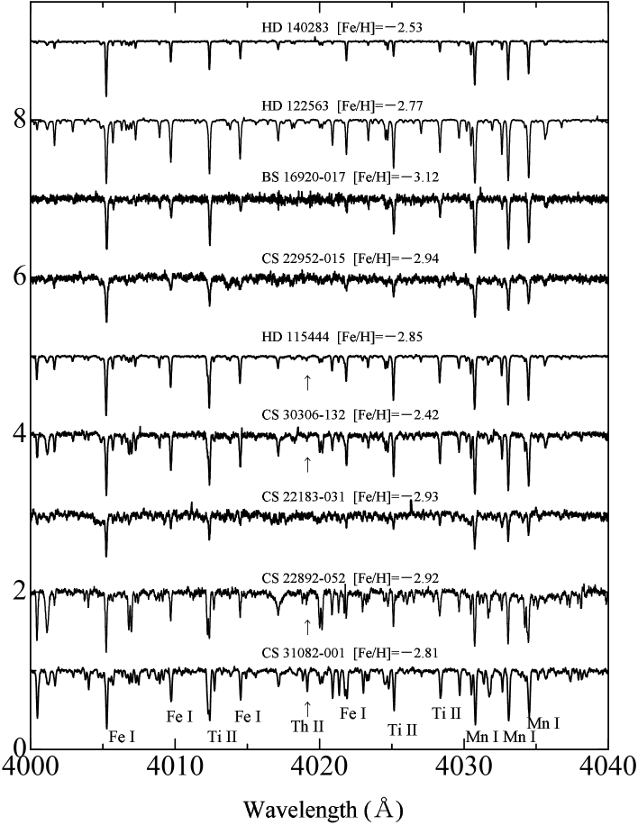
Figure 1: Examples of spectra for nine stars in our sample over the wavelength range 4000–4040Å. The star names and [Fe/H] values reported in Paper II are presented in the figure. This spectral region includes the line of Th II at 4019 Å; detections are indicated with a vertical arrow. The apparent emission lines seen in some of the spectra result from imperfect cosmic-ray cleaning.

Sample spectra for nine of our program stars in the regions near 4000 Å (which includes the Th II 4019 Å line) and 4100 Å (which includes the Eu II 4129 Å line) are shown in Figures 1 and  2, respectively. HD 140283 and HD 122563 are familiar, well-studied metal-poor stars. BS 16920–017 is the star with the lowest metallicity in our study, with [Fe/H] $=-3.1$. CS 22952–015 has been studied by previous authors (McWilliam et al., 1995b; Ryan et al., 1996). In the spectrum of CS 22183–031, the Eu II 4129 Å feature is detected, but it is quite weak. Given the paucity of information on the Eu abundances of stars with [Fe/H] $\sim-3.0$, this object should be re-observed at higher S/N in order to obtain a better measurement. The other four objects in these figures show enhancements of the r-process elements. CS 22892–052 and CS 31082–001 are well-known, extremely r-process-enhanced, very metal-poor giants (Sneden et al., 1996; Cayrel et al., 2001). These two objects clearly show the Th II 4019 Å line, as well as very strong Eu II 4129 Å features. HD 115444 is the object shown by Westin et al. (2000) to exhibit a moderate excess of r-process elements. CS 30306–132 turned out to exhibit excesses of the neutron-capture elements, as discovered during the present work. The Th II 4019 Å line was clearly detected in this object (see Paper II for details).

3 Equivalent Width Measurements

We identified Fe absorption lines between 3700 Å and 5100 Å, which will be used to determine the atmospheric parameters for the abundance analysis using model atmospheres. Identification of these lines was mostly made on the basis of the line list provided by Westin et al. (2000). Equivalent widths were measured for clear, unblended lines of Fe I and Fe II by fitting gaussian profiles to the observations using the spectral analysis software SPTOOL, developed by Y. Takeda (private communication). We excluded lines from our analysis that may be significantly blended with other absorption lines. The blending with other atomic lines was checked by using the atomic line list by Kurucz & Bell (1995).

Gaussian fitting may not well reproduce the wings of strong lines. However, for weak lines, the difference in derived equivalent widths from evaluations based on gaussian fitting and those based on direct integration over the observed line profile is very small. Since our analysis relies exclusively on weak lines, we measured all equivalent widths by the gaussian fitting procedure.

In addition to Fe lines, we also identified absorption lines of other elements, using the line lists provided by Westin et al. (2000) and Sneden et al. (1996). For Ba lines, we adopt the list of McWilliam et al. (1998). For La, Eu, and Tb lines, we take from the list of Lawler et al. (2001a,b,c). We use the newest data also for Nd and Yb which are derived by Den Hartog et al. (2003) and C. Sneden (private communication). Equivalent widths of these lines were also measured in the same manner as applied to the Fe lines. The measured equivalent widths are given in Table 3. The line data (lower excitation potentials, L.E.P., and the $gf$-values) are also listed in Table 3.

3.1 Estimates of Internal Errors

We estimate the random (internal) errors of our derived line strengths by determining the differences in measured equivalent widths from two measurements of each spectrum obtained with different individual exposures.

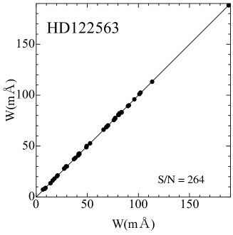
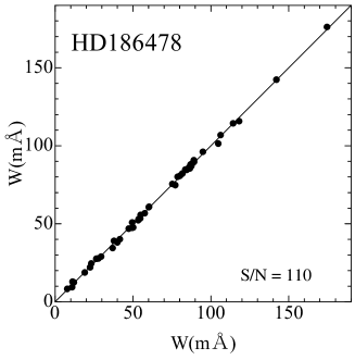
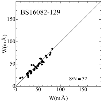
Figure 3: Comparison of equivalent width (W) measurements for spectra obtained by individual HDS exposures for HD 122563 (top), HD 186478 (middle), and BS 16082–129 (bottom). The S/N ratio of the final summed spectra are given in the individual panels. See text for details.

We selected three objects, HD 122563, HD 186478, and BS 16082–129, as representive of stars observed with high, moderate, and rather low S/N ratios, respectively. The number of photons collected by each exposure is about 70000, 12000, and 1000 at 4000 Å for HD 122563, HD 186478, and BS 16082–129, respectively. Comparisons between the two measurements of weak Fe lines for these three objects are shown in Figure 3. No systematic differences between the individual measurements are evident. The standard deviations in the differences of the two measurements for HD 122563, HD 186478, and BS 16082–129 are 0.39, 1.26, and 4.98 mÅ, respectively.

The uncertainly in the measured equivalent widths may also be roughly estimated, based on the S/N ratio of the spectrum, as (line width) $\times$ (S/N)^-1. The typical line widths for giant stars in our sample is 7.5 km s^-1 (100 mÅ at 4000 Å). The uncertainty expected from the S/N ratio of each spectrum, which is taken to be the square-root of the number of detected photons, is 0.38, 0.90, and 3.2 mÅ for HD 122563, HD 186478, and BS 16082–129, respectively. The random errors measured above show a reasonable agreement with these values, though the measured ones are slightly higher than those predicted from the S/N ratios. This small discrepancy may arise because the Fe lines used in our analysis are randomly distributed across individual orders, which have a blaze function variation in their S/N levels, while the number of photons was measured at the center of the echelle blaze profile.

3.2 Comparisons with Previous Studies

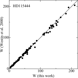
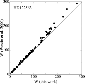
Figure 4: Comparison of equivalent width (W) measurements (mÅ) by Westin et al. (2000) and this work.

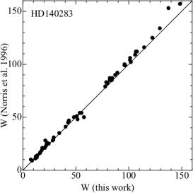
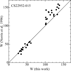
Figure 5: Comparison of equivalent width (W) measurements (mÅ) by Norris et al. (1996) and this work.

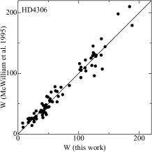
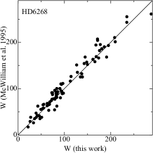
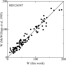
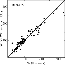
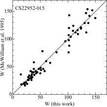
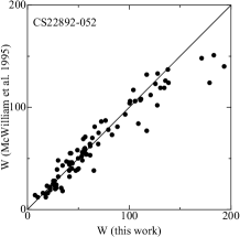
Figure 6: Comparison of equivalent width (W) measurements (mÅ) by McWilliam et al. (1995a) and this work.

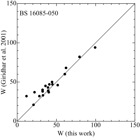
Figure 7: Comparison of equivalent width (W) measurements (mÅ) by Giridhar et al. (2001) and this work.

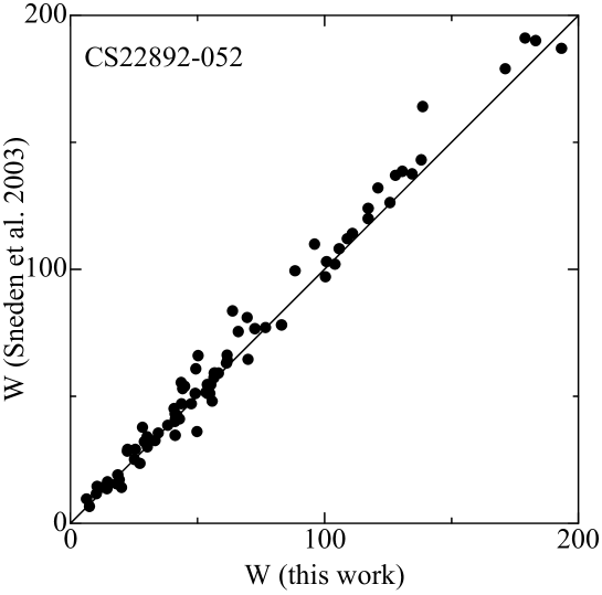
Figure 8: Comparison of equivalent width (W) measurements (mÅ) by Sneden et al. (2003) and this work.

Several stars in our sample have also been investigated by previous authors conducting high-resolution abundance studies. In Figures 4-8, the equivalent widths estimated from the present data are compared with those reported by others.

Westin et al. (2000) analyzed high-resolution ($R\sim 60,000$) and high S/N ($\sim$ 200 at 4000 Å) spectra of the two bright objects HD 122563 and HD 115444, obtained with the “2d-coud” cross-dispersed echelle spectrograph at the McDonald Observatory 2.7m telescope; their results are compared with ours in Figure 4. An excellent agreement is found, with a very small scatter ($\sim$ 2$\%$) in the range of equivalent width less than 150 mÅ. There is a small ($\sim 10$%) difference in the range of equivalent widths larger than 150 mÅ for HD 122563. The reason for this difference is not clear, but this difference does not have a significant influence on the abundance analysis because we are primarily concerned with weak lines.

Norris et al. (1996) obtained high-resolution spectra for two of the very metal-poor stars included in our sample, using the coude spectrograph (UCLES) at the Anglo-Australian Telescope. They studied spectra with $R\sim$ 40,000 of CS 22952–015 (S/N $\sim$ 50) and HD 140283 (S/N $\sim$ 200). In Figure 5, the equivalent widths measured for our spectra are compared with theirs for these two objects. The agreement is very good for HD 140283; there is no systematic difference, and the dispersion is quite small ($\sim$ 2$\%$). On the other hand, the scatter in the comparison for CS 22952–015 is larger, and our equivalent widths are systematically smaller than those of Norris et al. (1996) ($\sim$ 10$\%$) for lines with large equivalent widths ($>100$ m Å). The large scatter is presumably due to the lower S/N ratios in the CS 22952–015 spectra than those of HD 140283 in both studies. Most of the lines with equivalent widths stronger than 100 mÅ come from the portions of the spectra at wavelengths blueward of 4000 Å. We suspect that the discrepancy found for these strong lines is due to errors in the measurements by Norris et al. (1996), which were based on spectra of rather low S/N in this wavelength region.

In Figure 6, equivalent widths for HD 4306, HD 6268, HD 126587, HD 186478, CS 22952–015, and CS 22892–052, reported by McWilliam et al. (1995a), are compared with ours. Their spectra were obtained with the 2D-Frutti photon-counting imager at the Las Campanas 2.5m telescope. The typical S/N of the observations obtained by McWilliam et al. (1995a) is S/N $\sim 40$ with R $\sim$ 22,000 at 4800 Å. Their wavelength coverage extends from 3600 Å to 7600 Å. In spite of the large dispersion in the equivalent widths between these two set of measurements, which is surely due to the low S/N ratios in the spectra of McWilliam et al. (1995a), the equivalent widths of McWilliam et al. (1995a) exhibit no systematic difference with respect to ours. One exception is the comparison with four strong lines in CS 22892–052. We suspect that this deviation is due to errors in the data of McWilliam et al. (1995a), because these lines exist in the shortest wavelength regions, where the quality of the McWilliam et al. data is quite low.

In Figure 7, equivalent widths for BS 16085–050, reported by Giridhar et al. (2001), are compared with ours. Their spectra were obtained with the Apache Point Observatory’s 3.5m telescope and vacuum-sealed echelle spectrograph. Though the comparison shows a rather large dispersion, which is likely due to the low S/N of the spectrum reported by Giridhar et al. (2001), there is no systematic difference between the two measurements. Although they also reported the equivalent widths of CS 22169–035, there are only four iron lines which were observed by both studies. Therefore we do not show the comparison for this object.

Recently, Sneden et al. (2003) reported the results of a new detailed analysis of CS 22892–052. Their optical spectrum was obtained with Keck I/HIRES, McDonald 2.7m/2d-coude, and VLT/UVES. In Figure 8, we compare our measured equivalent widths for CS 22892–052 with theirs. There exists no systematic difference between the two measurements, and the agreement is better than that found in the comparison with McWilliam et al. (1995a) for the same star.

4 Measurements of Radial Velocities

Information on radial velocities and (where proper motions are available) on the space motion of stars of the halo is required to understand the structure and formation of the Galaxy. Precise radial velocity measurements are of particular importance for the moderately and highly r-process-enhanced, metal-poor stars, in order to check on their possible binarity, as this may impact the likely astrophysical site(s) of the r-process. For example, Qian & Wasserburg (2001) have suggested that the r-process-enhanced, metal-poor stars were produced by contamination from companions that underwent Type II SN explosions.

Measurements of radial velocities were made for selected clean iron lines used in the equivalent width measurements. The wavelengths of the lines were measured, then compared with the rest (laboratory) values. For the objects observed at two different epochs, measurements were obtained for each spectrum. The measured heliocentric radial velocities, and their estimated standard deviations, are listed in Table 2.

Measurements of radial velocities have been previously obtained by a number of authors for several stars in our sample. However, most of them were based on low- or medium-resolution spectroscopy (e.g., Bond 1980; Norris, Bessell, & Pickles 1985). We choose to compare our measurements with only the results of high-dispersion spectroscopy from recent studies. The comparisons are given in Table 3. No significant variation in radial velocity is found for most objects. HD 4306 and HD 186478 show changes of radial velocity of about 6 km s^-1 and 2 km s^-1, respectively, suggesting that both stars may be members of binary systems. Indeed, Carney et al.(2003) have obtained an orbital solution for HD 186478, showing it to be a long-period binary ($P\approx 550$ days) with a low amplitude, on the order of 3 km s^-1. No definitive conclusion can yet be achieved for HD 4306, hence further radial velocity monitoring is required to confirm its possible binarity. We note that HD 186478 is a moderately r-process-enhanced star, with [Eu/Fe] $\approx+0.5$ (Johnson & Bolte 2001). Preston & Sneden (2001) investigated the variations of radial velocity for the extremely r-process-enhanced star CS 22892-052 in detail. However, there is still no clear evidence of binarity, as the suspected amplitude of the variation is quite small. We did not find evidence of binarity for any of our other r-process-enhanced stars.

5 Summary

We have obtained high-resolution, high-S/N ratio, spectra for 22 very metal-poor stars with Subaru/HDS, taken during the commissioning phase of this instrument. These stars were selected so as to include as many objects with known (or suspected) enhancement of r-process elements as possible. In this paper we have reported the measurements of equivalent widths for isolated absorption lines in the reduced spectra, and also precision radial velocities (in some cases, at several epochs), for each star. Comparisons of our measured equivalent widths with previous work demonstrates that there exists no systematic differences, except in the cases of stronger lines in a few objects for which the S/N ratios of the previous work was rather low. In the following papers of this series (Paper II, others in preparation), the results of the detailed abundance analysis for these data will be presented.

Table 1: PROGRAM STARS AND OBSERVATION LOG

No	Star	$V$	$B-V$	$R$	S/Na	S/Nb	Exp.(sec)
1	HD 4306	9.08	0.63	90000	272	497	1800
2	HD 6268	8.10	0.79	90000	158	288	1800
3	HD 88609	8.59	0.93	90000	62	113	2110
4	HD 110184	8.31	1.17	90000	221	403	900
5	HD 115444	8.97	0.78	90000	255	466	3900
6	HD 122563	6.20	0.91	90000	374	683	1200
7	HD 126587	9.15	0.73	90000	187	341	4500
8	HD 140283	7.21	0.49	90000	458	836	3600
9	HD 186478	9.18	0.90	100000	158	274	2400
10	BS 16082–129	13.55	0.67	50000	55	135	5400
11	BS 16085–050	12.15	0.74	50000	100	245	5100
12	BS 16469–075	13.42	0.77	50000	59	145	5400
13	BS 16920–017	13.88	0.76	50000	41	100	5400
14	BS 16928–053	13.47	0.85	50000	49	120	5400
15	BS 16929–005	13.61	0.62	50000	56	137	5400
16	BS 17583–100	12.37	0.51	50000	79	194	3600
17	CS 22169–035	12.88	0.92	50000	49	120	5400
18	CS 22183–031	13.62	0.65	50000	47	115	9751
19	CS 22892–052	13.18	0.78	90000	60	147	7200
20	CS 22952–015	13.27	0.78	50000	59	145	9000
21	CS 30306–132	12.81	0.80	50000	85	208	4493
22	CS 31082–001	11.67	0.77	50000	100	122	1200

^a S/N ratio per pixel at 4000 Å.

^b S/N ratio per resolution element at 4000 Å.

Table 2: COORDINATES AND RADIAL VELOCITY

No	Star	R.A. (J2000.0)	Dec. (J2000.0)	Obs.Date	Vr a
1	HD 4306	00 45 27.2	$-$09 32 40	19 Aug, 2000	–69.69$\pm$0.29
2	HD 6268	01 03 18.2	$-$27 52 50	18 Aug, 2000	39.20$\pm$0.27
3	HD 88609	10 14 29.0	+53 33 39	11 nov, 2000	–37.28$\pm$0.43
4	HD 110184	12 40 14.1	+08 31 38	29 Jan, 2001	138.89$\pm$0.27
5	HD 115444	13 16 42.5	+36 22 53	4 July, 2000	–27.30$\pm$0.34
5	HD 115444			28 Jan, 2001	–27.58$\pm$0.25
6	HD 122563	14 02 31.9	+09 41 10	4 July, 2000	–27.20$\pm$0.33
6	HD 122563			29 Jan, 2001	–26.52$\pm$0.34
7	HD 126587	14 27 00.4	$-$22 14 39	27 Jan, 2001	148.72$\pm$0.72
7	HD 126587			31 Jan, 2001	149.10$\pm$0.24
8	HD 140283	15 43 03.1	$-$10 56 01	4 July, 2000	–171.17$\pm$0.29
8	HD 140283			17 Aug, 2000	–170.23$\pm$0.19
9	HD 186478	19 45 14.1	$-$17 29 27	20 Aug, 2000	30.52$\pm$0.31
10	BS 16082–129	13 47 11.5	+28 57 46	30 Jan, 2001	–92.16$\pm$0.30
11	BS 16085–050	12 37 46.7	+19 22 44	31 Jan, 2001	–75.06$\pm$0.28
12	BS 16469–075	10 15 10.1	+42 53 19	28 Jan, 2001	332.88$\pm$0.74
13	BS 16920–017	12 07 17.1	+41 39 35	27 Jan, 2001	–206.53$\pm$0.84
14	BS 16928–053	12 22 28.1	+34 11 24	28 Jan, 2001	–81.00$\pm$0.35
15	BS 16929–005	13 03 29.4	+33 51 06	30 Jan, 2001	–51.29$\pm$0.43
16	BS 17583–100	21 42 27.8	+26 40 34	19 Aug, 2000	–107.96$\pm$0.32
16	BS 17583–100			20 Aug, 2000	–108.76$\pm$0.42
17	CS 22169–035	04 12 13.9	$-$12 05 05	11 Nov, 2000	17.72$\pm$0.73
18	CS 22183–031	01 09 04.9	$-$04 43 25	10 Nov, 2000	11.67$\pm$0.67
18	CS 22183–031			11 Nov, 2000	11.97$\pm$0.56
19	CS 22892–052	22 17 01.5	$-$16 39 26	22 July, 2001	12.72$\pm$0.49
20	CS 22952–015	23 37 28.6	$-$05 47 56	11 Nov, 2000	–20.07$\pm$0.71
21	CS 30306–132	15 14 18.6	+07 27 02	26 July, 2001	109.01$\pm$0.31
22	CS 31082–001	01 29 31.2	$-$16 00 48	30 July, 2001	138.91$\pm$0.30

^a Heliocentric radial velocity (km s^-1).

Table 3: EQUIVALENT WIDTHS FOR PROGRAM STARS: FIRST SAMPLE

Wavelength	Species	L.E.P.	$\log gf$	Equivalent width (mÅ)a
(Å)		(eV)		1	2	3	4	5	6	7	8	9	10	11	12	13	14	15	16	17	18	19	20	21	22
3829.35	Mg I	2.71	–0.480	157.6	198.5	156.4					125.3		131.5	158	131.2	110.3	151.6	109.4	125.2	154	131.5	140.6	96.5	172.5
3832.31	Mg I	2.71	0.145	190.1	213.5	160.4	263.1	181.6	230	174.9	153.2	231.7	143.4	177	137.9	103.6	142.5	120	142.2	124.4	122.6	158.7	103.9	208.8	191
3838.30	Mg I	2.72	0.414	237.7	261.9	194.9		205.4	262	202	173.5	288.8	166.2	198	163.7	137.1	171	127.9	164.7	156.6	143.7	176.2	120.5	265.3
4571.10	Mg I	0.00	–5.569	45.5	77.4	76.5	132.6	51.7	85	43.8	7.7	95.7	32.2	42.2	24.1	17.5	49	15.4	10.9	49.7	21.6	27.4	17.1	59.2	55.3
4703.00	Mg I	4.35	–0.377					54.6	72	52.6	41	90.7	45	56.5					39.9		38.2	41.5	23.7	74.3	61.9
5172.70	Mg I	2.71	–0.381						209	168.4			150.4	176.8		131.6						154.5		193	187.3
5183.62	Mg I	2.72	–0.158						232	187.1			169.6	192.4		149.7						177.4		231.7
3961.53	Al I	0.01	–0.336	106.9	139.5	118.1	174.3	112.4	146	104.6	68.4	145.3	88	105	85.5	85.1	97.5	64.2	67.1	101.6	81.4	107	93.2	119.1	110.2
4102.94	Si I	1.91	–3.100	63	91.4	76.6	114.5	57.4	82	60.5	19.4	89	46.8	73.2	40	22.9	56.1	18.2	15.5	68.3	40.1	44.6	45.6	68.5	66.9
4226.73	Ca I	0.00	0.240																134.9			syn
4283.01	Ca I	1.89	–0.220					46.5	65.6	52.2	29.6	84		39.5	35.5	12.8	44.2	30	28		16.5		18.3
4318.66	Ca I	1.90	–0.210	47.4	64.1	43.9	81.4	40.9	55.4	40.6	27.2	69.9	37.2	36.8	24.9	25.2	40.1	18.8	26.7		19.3	32	26.8	54.4	48.7
4425.44	Ca I	1.88	–0.358	42.7	55	39.9	71.6	34.4	49.1	35.7	22.2	63.5	33.9	31.4	29.2	11.2	41.8	20.7	22.4		19	35.2		52
4454.79	Ca I	1.90	0.260	70.3	95.4	69.5		64.9	79.9	64.6	48.5	97.1	57.9	60.7	42.6	30.8	61.7	35.1	43.9		49.9			81
4455.89	Ca I	1.90	–0.510			35.4							24.2						17.5			25
4400.40	Sc II	0.60	–0.540	56.2	86.6	67		58.2	78.3		17.5	79.6							13.5		30.5		32.3
4415.56	Sc II	0.59	–0.670	48.9	78.1	61.7	103	52.2	76	47.7	14.7	80.9	37.4	51.4	29.1	29.2	41.1	3.7	13.1	46.6	22.8	41.4	23.5	50.7
5031.02	Sc II	1.36	–0.400	20.3	46	30.2	64.7	22.3	42	18.5	4.8	47	17.3	27.1	12.3	8.4	21.9			20.3		15.3		26.2	21.8
3998.64	Ti I	0.05	–0.056	54.8			108.8	56.5	70.2	52.3	24.2	81.5	43.3	38.3	28		53	26.2	23.3		32.8	37.7	33.2	59.4	59.2
4533.25	Ti I	0.85	0.476	38.6			84.6	40.9	52.2	35.5	14.4	63.4	29.1	24.8	20.6	30	36				54.3	25.3	23	47.5	104.4
4534.78	Ti I	0.84	0.280			36.5	71.8	31.1	42.6	95.5		54.7	23.4	17.6	16.1	19.3	30.9	14.1	10.6	36		21.6		38.1	32
4535.58	Ti I	0.83	0.130					24.2	35.6	21.2		49	18.8	12.4		14.7	29.9	10.5				15.1		30.7	27.2
4981.74	Ti I	0.85	0.504	44.5	66.7	51	97.5	47.2	61.6	39.8	19.1	73.3	36.9	31	25	39.2		16.7	19.4	36.7	22.5	31.5	15.9	54.7	48.9
4991.07	Ti I	0.84	0.380	40.7				42.1	57.8	37.7	16.4	71	34.1	24.5	22.4	17.8	39.7	16		36.6	16.1	29.1		49.5	44.8
4999.51	Ti I	0.83	0.250	35.8	57.3	40.4	86.1	36.3	49.1	31.6	12	64.3	23.2	21.7	16.4	25.3	31	13.6	15.1		16.7		12.8	42.2	47.3
5039.96	Ti I	0.02	–1.130	17.3		22.7	72.1	18.9	30.2	15.9	3.3	45.3	13.8	10.5	10.5	12.8	14.9					9.7		20	20.6
5064.66	Ti I	0.05	–0.991	20.5		29.9	78.9	22.5	35.9	18	5	49.3	10.8	11.1	11.3		22.3					12.4		27.9
5173.75	Ti I	0.00	–1.118				76.3		34	16.6				8.8	8.1	14.8	20.2							22.1
5192.98	Ti I	0.02	–1.006						39.2	19.7			17.9	11.5	10.7	15.5	18.7	7						28.8
4028.35	Ti II	1.89	–1.000	38.4			82.2	42.1	52.5	35.4	13.4	70.9	27.7	25.2	21.8	26.8	33.5	12	11.3		16.8		22.4	45.8
4337.93	Ti II	1.08	–1.130	84.5	119	80.4	145.1	92.8		78	40.9	110.1				70.2			37.4	69.6	47.5		50	81
4394.07	Ti II	1.22	–1.590	42.3	70	55		48.1			11.5	74.9							12.2
4395.85	Ti II	1.24	–2.170	30.6	57.8	122.6		36.2	46.6		6.7	58.1								103.4	64.8
4399.78	Ti II	1.24	–1.270	74.5	96.6	81.4		75.4	89		30.5	102.5							29	53.7	42.4		35.9
4417.72	Ti II	1.17	–1.430	73.9	105	88.6	129.5	81.1	95.1	70.6	32.3	104.1	62.2	60.2	52.6	63.4	69.4	29.4	28.8	67.6	34.4	65.7	41.4	86.5
4443.81	Ti II	1.08	–0.700	96.8	128.2	116	160.1	104	119.3	95.7	60.8	126.7	85.4	90.2	76.3	87.7	100.8	55.3	57.7	91.6	61.1	84.7	73.3	100.6	101.9
4450.49	Ti II	1.08	–1.450	64.7	96.6	75.6	124.7	71.5	87.4	63.8	23.8	92.5		54.3	43.2	58.1	65.8	23.8	21.6	52.3	34.7	50.9	33.9	68.5	68.9
4464.46	Ti II	1.16	–2.080	44.8				50.2	67	42.9	11.7	76.5	35.9	32.6	22.7	38.5	45.8	18.3	12.7			30.5		50.5	47.1
4468.50	Ti II	1.13	–0.600	98.4	132.5	112.8	163.8	107.1	121.4	98.1	63.1	130.6	83.7	90.6	78.3	89.3	101	59.6	60.3	88.6	57.8	93.3	70.9	102.4
4470.86	Ti II	1.17	–2.280	28.1	56.8	38.1	74.9	34.1	48.6	26.6	5.4	59.3	22.4	18.9	16.6	24.5	27.3							34.6
4501.28	Ti II	1.12	–0.750	93.9		109.8	156.1	101.7	117.2	93.1	57.2	125.3	82.7	86.3	70.7	83	95	55.6	54.2	92.5	60.7	83.2	69.9	97.9	98.5
4571.98	Ti II	1.57	–0.530	85.8			154.6	92.6	109.9	84.5	52.6	117	74	80.5	64.4	76.8	87.9	44.7	49.2	85	49.1	77.2	62.1	92.2	92.3
4589.95	Ti II	1.24	–1.790	48.4		61.5	102.4	54.3	71.7	46.4	13.9	78.9	40	34.3	26.2	41.6	48.5	10.2	12.5	47.9	18.4	34		52.4	55.4
4865.62	Ti II	1.12	–2.610	11.3	29.7	20.9	51.8	15.1	25.2	11.5	2	32.3	12	9.8			22					11.1		14.7
5129.16	Ti II	1.89	–1.390				72.6		45.1	22.8			23.2	17.2	12.9	20.6	24.9					18.4		31.6
5185.91	Ti II	1.89	–1.350				65.6		37.1	19			16.5	15.4	11.1	17.9	22.6					11.8		27.1	22
5188.70	Ti II	1.58	–1.210						90	59.8					34	49		19.2
4379.24	V I	0.30	0.565	14.2	28.9			14	28		4.9	38.6											11.6
4389.99	V I	0.28	0.235					8.7	21.7
3951.96	V II	1.48	–0.784	17.7	44.6	34.9		21.6	35.4	17.4	5.2	42.5	36.1	18.2	11.6		16.2		6.2		17.1	15.7		23.3	29.4
4005.71	V II	1.82	–0.522	18.1	46	38.6		19.3	36.3	18.4	5.2	43.5	16.9	17.6	7.1	17.6	21.1							23.2	33.5
4254.35	Cr I	0.00	–0.114						113.7	88	66.3		84.2	83.7	70.7	82.9	95.6	52.4	60.1			87.4		96.8	95.7
4274.81	Cr I	0.00	–0.231						112.8	88.1	63.5		82.2	79.4	69.1	79.6	92.5	52.9	53.6		51.3				96.7
4289.73	Cr I	0.00	–0.361	85.9	109.8	92.1	135.1	86	109.1	82	57.2		76.8	72.6	67.2	72.9	88.3	47.6	49.6	88.1	53.1		66.4	96.1
4554.99	Cr II	4.07	–1.380					2.8	4.8	4.8	1.5
4558.65	Cr II	4.07	–0.660	10.2	30.2	13.4		11.1	20.7	20.7	8.7	28.2	9.8	11.2		8.9	12.2							17.9
4588.20	Cr II	4.07	–0.630	8.4	19.8	6.8	23.5	7.1	13.3	13.3	5	18.6	5.2	5		4.1	7.9							9
4030.76	Mn I	0.00	–0.470	91	138.2	105.5		97.2	140.8	97.2	66.8	138.8	84.8	106.1	75.5	98.7	97.1	39.5	50.4	130.3	65.1	93.6	91.6	109.8	109
4033.07	Mn I	0.00	–0.618	77.4	124.4	95.8	179.3	83.6	125.2	83.6	55.2	124.9	75.1	91.6	61.3	86.7	91.9	35.6	38.9	112.2	46.3	92.2	73.2	97.8	96.2
4034.49	Mn I	0.00	–0.811	79.1	105.8	89.3	164.8	75.2	119.8	75.2	45.9	121.3	77.1	80.9	57.7	80.8	86.7		33		36.4		57.4	108.1	91.8
4041.37	Mn I	2.11	0.285	16.6	45.7	37.2	67.7	15.7	43.9	15.7	13.3	47.1	23.2	26.6	7.7	31.8	26.6					18.7		30.8	19.8
4754.04	Mn I	2.28	–0.086	6.3	18.1	11.6	40.6	5.9	19.9	5.9	5.2	21	6.5	9.7		13.5	13.2					5.5		12.3	7.3
4823.51	Mn I	2.32	0.144	8.8	26.2	12.8		8.6	25.7	8.6	7.3	28.4	11.3	14.9		13.3	14.3							20.1
3763.80	Fe I	0.99	–0.221	139	209.9			152.4	171.7	138.7	107.8	217.1	113.9	131.3	116.6	98	137.2		103		102.5	134.5	53.9	155	140.4
3767.20	Fe I	1.01	–0.382	125.9	175.7			137.6	151.7	127.3	96.9	180.3	106.1	120.7	110.8	90.8	128.9	83.8	86.4		84.4	127.6	109.2	137.8
3787.89	Fe I	1.01	–0.838	112	148.2	116	222.8	131.1	129.7	110.3	84.5	145.9	89.4	108.4	100.5	85.3	115.7	72	80.9	130.3	63.7	109	51.2	114.8	109
3805.35	Fe I	3.30	0.313	46.8	78.8		81.6	58.1	59.3	48.9	40.4	76.9	52.1	42.3	42.7		47.8	19.2	34.3		31.2	65.3	47.4	63.6
3815.85	Fe I	1.49	0.237	137.2	191.1			150.9	165.6	138.1	114.6	195.1	119.6	131.5	121.5	96.9	138.2	91.8	109		111.1	138.7	102.5	156.6	164
3820.44	Fe I	0.86	0.157	188.2	287.4	252.6		210.3	279.7	193.3	148.5	331.7	168.2	172.2	159.9	149.9	210.2	122	134.8		143.3	183.2	149.6	234	210
3825.89	Fe I	0.92	–0.024	165.1	234.8	198.3		182.3	222.2	165.8	129.4	272.9	151.6	152.4	134.5	131	180	107	119		125.5	171.2	135.5	193.3
3827.83	Fe I	1.56	0.094	124.3	177.5	117		136	159	124.5	102	185.9	112.5	122.1	97.8	107.9	137.8	84.4			89.7	127.6	101.5	140
3840.45	Fe I	0.99	–0.497	123.9	171.5	138.8		136.6	154.4	126.7	96.1	182.8	109.9	121.7	111.7	92.1	130	82.2	91.7		88.9	121.1	109.8	139	129.4
3849.98	Fe I	1.01	–0.863	110.6	149.7			125.2	142.2	111.9	87.3	156.4	103.7	111.7	101.2	99.5	124.7	82.3	80.3		78.6	117.3	105.2	119.1	119.9
3856.38	Fe I	0.05	–1.280	137.6	180.7	160.6		155.8	173.6	140.3	106.1	189.3	117.6	139.6	117.5	123.1	148.7	96	98	155.9	101.5	138.1	138.9	146.4	149
3859.92	Fe I	0.00	–0.698	184	234.7	203.7		190.7	238.2	185.3	137.5	292.4	151.9	168.5	156	142.5	195.6	116.1	126.6	182.3	121	179	144.1	215.2	191.1
3865.53	Fe I	1.01	–0.950	111.2	144.8	115.9	194.6	119.6	136.1	111.7	84.1	148.2	100.7	110.3	100.9	90.4	117.7	72.5	78.7	128.6	82.2	111.1	102	115.8	118.7
3886.29	Fe I	0.05	–1.055	115.4	208.5	161.7		165.3	184.7	156	109	221.3	127.6	141.4	144.7	125.8	150.4	103.5	105.5	174.1	104.8	193.4	132.8	179.6	173.3
3899.72	Fe I	0.09	–1.515	127.7	165.9	150.1		140.5	162.5	129.6	96.7	168.2	121	133.8	122.7	118	140.5	93.8	93.3	158.4	91	130.7	133.3	132.7	139.3
3902.96	Fe I	1.56	–0.442	103.8	138.9	118.5		112.1	131.4	105.5	82.2	123.5	98.2	103.5	89.1	92.4	111.8	68.8			76.3	105.9	11.3	111.3	108.1
3920.27	Fe I	0.12	–1.734	121.8	161.7	142.5		137	157.7	123.1	89.3	161.7	119.8	122.6	115.9	114.1	137.1	88.4	84.6		99.5	125.8	118.2	121.8	126.2
3922.92	Fe I	0.05	–1.626	128.9	171.7	148.1	253.8	142.5	168.4	132	96.1	173.5	124.2	132.4	120.6	114.2	148.2	95.1	91.4	164.3	93.6	128	130.3	135.7	133.5
3949.96	Fe I	2.18	–1.251	45.5	68.5	61	95	47.7	66.9	44.9	28.3	73.8	37.2	36.1	30.8	26.8	48.1	16.5	23.2	59.4	36.9	42.9	30.1	55.9	50.7
4005.25	Fe I	1.56	–0.583	101.5	142.7	110.1		110.4	131.7	103.1	78.8	142.4	98.8	99.4	87	85	112	67.2	71.5		81.8	100.4	102.5	104.7	107.5
4063.61	Fe I	1.56	0.062	128.4	186.3	147.7		139.4	166.3	129.6	106.7	179.9	118.6	127.5	115.9	110.3	137.6	88.3	96.5		110.1	135.7	123.7	144.9
4071.75	Fe I	1.61	–0.008	120.6	168.7	150		130.1	153.7	120.8		171.2	109.6	117.3	107.4	72.6	115.7	80.9	91.7		76.9	117.3	113.8	130.9	128.7
4076.64	Fe I	3.21	–0.528	26.7		25.8		29.4	45.1	27.2	18.5	59.8		21.9				16	15.5			34.6		39.4
4114.45	Fe I	2.83	–1.303	12.8	33.3	16.8	52.8	14.3	28.8	13	8.7	38.9	19.6	10.7			16.7					10.2	17.4	18.8	16.6
4132.91	Fe I	2.85	–1.005	23.1	47.2	119.5	184.4	22.7	42.2	102.7	15.3	143.8	90.2		87.2		24.7		17.3		67.3	101.6	95.4	33.8
4134.69	Fe I	2.83	–0.649	36.3	66	48		43.8	58.3	38	28.2	68.6	37.1		21.4		37.8	15.7	21.3		18.5	34.6	33.8	53.6	48.9
4143.88	Fe I	1.56	–0.511	104	134.7	123.9		113.2	134.5	104.8	83.7	135.3	100.1	105.5	94.4	102.3	117.5	75.9	81.9		72.5	104.2	101.3	111.1	50.4
4147.68	Fe I	1.49	–2.071	47.5	82.1	64	112.5	57.5	78.7	49.5	22.5	85.5	46.6	40	35.3		59.9	18	15.2		15.7	49.2	35.6	58.7	57.9
4154.51	Fe I	2.83	–0.688	38.1	49.4	36.9		32.1	52.4	23	21.3	64.7	27.2	24			36.2		21.5					51.9
4156.81	Fe I	2.83	–0.808	39.6	63	37.5		34.5	59.3	33.6	22.5	69.2	29	27.1	17.9		37					28.5		46.1
4157.79	Fe I	3.42	–0.403	27.8	38.8	24	58.2	22.2		22.7	13.9	57.7	19.7	15.6	17							29.2		35.6
4174.92	Fe I	0.92	–2.938	41.9	76.2	70.2	130.4	58.1	78.6	44.7	14.3	84.6		31.9	25.7	30.9				66.9		45	33.8	57.3	53.8
4175.64	Fe I	2.85	–0.827	30.1	66.2	41.8	78.9	42.4	52.5	31.1	20.9	64.5		20.9				14.8	17.7			41.3	20.1	45.6
4181.76	Fe I	2.83	–0.371	53.2	79.5	57.2			69.8	50.5	38.7	84.2	47.1	41.2	38.8		53.5	25.2				56.5		59.6	57.2
4182.39	Fe I	3.02	–1.180	8.6	25.9	10.2	40.9		18.9	10.2	5.7	27.5												15.6
4187.05	Fe I	2.45	–0.514	64.7	91.4	77.4	123.5	82.7		64	51.7	94.1	53.6	55.9	51.5	44.4	74.2	31.8	38.7	86.7	35.3	61.8	55.4	74.1	71.8
4187.81	Fe I	2.42	–0.510	66.5	97.9	77.1		70.4		69	57.8	103.1	63.7	59.6	55	54.6	73.5	38.3	40.6		31.7	69.6	57.8	80.6	75.7
4191.44	Fe I	2.47	–0.666	54.7	90.3	61.6		59.2	79.5	56.8		84.8	51.7	50.8	41.3	41.8	62.1	22.7	32.9			55.3		69.2	68.8
4195.34	Fe I	3.33	–0.492	30.5	39.3	25.5	73.7	30.3	43	27.7	16.6	56.4	28.7	17.3	17.3		28.3		16					41.4	32.3
4199.10	Fe I	3.05	0.156	61	85.3	74.3		63.7	80.9	60.4	48.3	90.2	56.2	53.6	47.5	38	63.7	32.2	43.1	78.1	28.3	72.7	51.3	70.6	74.2
4202.04	Fe I	1.49	–0.689	102.3	137.5	113.1		110	132.1	104.6	80.2	126.2	99.4	101.3	90.3	94.2	112.2	72.4	76.3	140.3	73.7	100.9		106.7	115
4222.22	Fe I	2.45	–0.914	45.6	74.4		101.9	48.6	73.4	47.3		78.6	46.6	40.3	32.7	29.9	58.1	20.1		66.2	25.9	40.8	30.1	59.2	60.1
4227.44	Fe I	3.33	0.266		93.7	88.3		64	96	59.6	42.8		53.8	49.4	39.7	40.2	67.7	28.8				54	38.4	76.9	68.8
4233.61	Fe I	2.48	–0.579				119.7		85.9	60.5	43.5		57.2	54.6	45.3	58.9	66.7	29.5				58.3		73.4	68.3
4250.13	Fe I	2.47	–0.380				123.3		96.3	70.1	53.8		61.7	62.3	53.8	46.7	74.7	34.5				63.8		78.2	83.5
4250.80	Fe I	1.56	–0.713				166.2		129.9	100.6	77.8		98.8	98.1	89.8	87.6	108.5	62				96.1		105	109.8
4260.49	Fe I	2.40	0.077						122.6	95	77.9		88.2	91	79.1	79.9	98.3	55.7				88.5		100.7	99.4
4271.16	Fe I	2.45	–0.337						106.9	82.8	55.4			70.5	64.8	118.9	84.3	54.8						101.2
4325.77	Fe I	1.61	0.006	125.6	173.9	150.7		134	163.3	130.9	101.3	180.7		124		123.8	140.8	89	97.4		97.5		123.7	146.3
4337.06	Fe I	1.56	–1.704	62.1	94.1	74.1	136.2	69.4	88.9	65.5	32.8	93.5			49.6				32.7		40.1		44.6	76.3
4383.56	Fe I	1.49	0.208	143.6	195.1	175.6		151.5	188.2		122.4	199.3							111.8	178.7			136.9
4404.76	Fe I	1.56	–0.147	123.3	168.1	146.1		130			101.2	171.2							94.5	161.5	90.3		117.5
4415.14	Fe I	1.61	–0.621	104	126.4	126.5		109	134.8	108	82.2	136.7		102.2	94	100.3		69.6	76.7	135.6	82.3	111.7	101.7
4430.62	Fe I	2.22	–1.728	26.7	55.7	39.1	86.5	31.3	54.7	27	13.8	61.8	28		19.2		39.1					26.9	22.4	40.1
4442.35	Fe I	2.20	–1.228	49.3	82.2	66.7	118.1	52.7	78.8	51.8	29.2	88.7	52.8	41	36.6	32.8	59.7	19	22.4		32.8	61.7	34.8	68.1	66.2
4443.20	Fe I	2.86	–1.043	18.9	41.3	33.7		18.7	37.4	19.2	12.3	47	19.9	14.3	13		25.2		9.1			15.3	18.2	29.4
4447.73	Fe I	2.22	–1.339	44.7	74.2	62.4	104.6	45.6	72.6	44	24.5	80.4	42.1	35.6	27.6	23	53.5	17.1	16.8		21.2	44.2	33.9	57.8	52.9
4466.56	Fe I	2.83	–0.600	49.3	83.6	71.8		54.7	84.5	50.7	28.9	90.3	48.8	41	36.2	28.6	63.7	19.3	23.4		29.9			65.1	62.4
4489.75	Fe I	0.12	–3.899	40.3	82.1	82.8	136.2	52.8	84.9	46.1	11.6	85.9	44.1	35.1	32.5	5.6	64.3		9			43.6	26.2	56.4	55.3
4494.57	Fe I	2.20	–1.143	54.9	85.8	70.2	120.5	60.3	82.9	55.7	34.5	88	51.4	44.5	43.9	41.6	64.9		27.4	68.8	31.5	50.3	35.2	65.8	65.9
4528.63	Fe I	2.18	–0.887	71	112.9	90.6	153.3	77.4	103.3	73.4	51	114.9	65.9	63.5	55.1	57.2	76.4	32.6	42.8	90.8	40.7	79.5	60.7	89.6
4531.16	Fe I	1.49	–2.101	48.9	82.4	68	127	55.8	82.6	50.6	21.9	87.6	47.5	39.3	37.4	31.7				70.1	25.3	49.4	38.3	63.1	60.7
4602.95	Fe I	1.49	–2.208	46.3	81.2	71.6	121.1	53.1	80.1	48.4	20.2	27.2	44	39.1	32.8	30.8	60.7	22.3	19.8	65.9		43.7	32.7	59.8	57
4736.78	Fe I	3.21	–0.752	23.1	45.6	32.7	72.6	23.4	43.1	22.5	14.2	53.9	24.4	16.8	16	12.2	24.6	14.4		38.8		22.5		33.2	29
4871.32	Fe I	2.87	–0.362	51.2	82.5	64.5	107.9	55.7	79	52.3	36.3	86.5	54.6	44.4		37.6	59.5	23.5	33.2	69.2	33.1	54.9	39.2	65.2	63.8
4872.14	Fe I	2.88	–0.567	41.5	71.9	55.6	99.8	45.6	67.7	42.8	27.1	75.8	44	32.9		29.7	46.3	21.7	27.4	56	21.3	41.3	29.1	53.6	54.3
4890.76	Fe I	2.88	–0.394	51	84.5	62.3	109.2	54.9	77.8	50.6	35.7	86.7	50.5	44.3	33.1	32.3	60.4	19.4	30	69.8		56.9	37.6	65.2
4891.50	Fe I	2.85	–0.111	64.5	93.2	79	121.4	67.8	91.6	64	49.5	97.7	66.6	58.7	46.5	48.8	71.4	30.8	43.7	80.5	42.3	61.5	50	76.8	74.1
4903.32	Fe I	2.88	–0.926	25.6	55	37.4	80.7	28.4	50.4	26.8	15.9	57.2	27.3	20	17.4	15.3	29.8		15	41.6	18	25.2	21.9	40.8	35.3
4919.00	Fe I	2.87	–0.342	52.7	83.7	66.9	110.7	56.4	78.9	53	38.2	86.9	54	44.9	39.5	37.1	62.6	28.7	33.2	65.1	30.8	55.8	42.5	68.3	64.2
4924.77	Fe I	2.28	–2.200	10.1	29.1	23.6	60.3	14.5	29.7	11.8	4.1	36.2			7.6					19.8		10.6		19	19.3
4938.82	Fe I	2.88	–1.077	18.5	45.6	32.1	72.3	22.4	42.8	21.8	11.7	51.8	22.8	16	9.9	12.3	31.9	5.9				20.1	16.5	35.2	26.4
4939.69	Fe I	0.86	–3.252	30	67.8	63.1	117.4	37.9	70.7	33.6	8.6	77.1	32.4	26.6	17.8	20.8	50			55.9			21.2	47.1	39.8
4946.39	Fe I	3.37	–1.010	7.2	19.6		35.3	6.8	16.5	7.4	3.9	21.4												15.9
4966.09	Fe I	3.33	–0.840	13.9	34.5	21.7	56.2	15.4	31.1	14.5	8.2	39	14	10.8		8.7	20.8					12	11.2	23.9	17
4973.01	Fe I	3.96	–0.850	3.8	9.3	3.2	16.8	4.6	9.7	3.3	2.7	9.8
4994.14	Fe I	0.92	–2.969	39.8	79.4	70.5	127	50.1	81.9	43	13	83.3	42	31.8	27.8	31	59.9	17.4		60.3	18.8	41.4	32.3	50.7	56
5001.87	Fe I	3.88	0.050	16.6	35.7	24.2	51.1	15.4	30.3	16.3	13.2	40.3	17.3	6.1	10.8	10.6	23.9	9.1	14.3	29.3		18.1		28.8	20.2
5006.12	Fe I	2.83	–0.615	42.5	73	58.6	101.7	45.2	70	43.1	27.2	78.8	39.3	33.5	28.8	28.4	49.8	15.5	23.4		23.6	41.1	27.5	57.6	51.4
5014.94	Fe I	3.94	–0.270	10.2	23.7	12.2	37.5	13	22.5	10.1	8	26.7		11.1			13					6.4		16.2	13.3
5022.24	Fe I	3.98	–0.490	6.4	16.3	9.8	26.5	8.5	14.4	7.4	5.6	18.9												14.5	6.2
5041.76	Fe I	1.49	–2.203	52.1	95.3	82.4	141.9	56.1	91.7	53.8	22.1	101.4	53.5	47.1	36.4	33.2	61.7	19.7	22.8		25.7	49.8	30.6	67.6
5044.21	Fe I	2.85	–2.040	3.8	11.4	6.7	23.1	5.1	9.9	3.5	1.7	11.2
5049.83	Fe I	2.28	–1.355	39.5	73.2	62	109	43	72.3	42.2	21.5	79.4	40.4	32.5	25.3	27	49.8	13.3	20.4	54.9	21.9	38.3	24	56.4	51.8
5051.64	Fe I	0.92	–2.764	56.9	96.7	90.5	145.8	67.1	97.6	61.4	23.9	101.8	57	51.7	41.5	44	76.7	21.3	21.7	83	32.2	56.6	41.6	71.4	71.6
5068.77	Fe I	2.94	–1.041	17.1	42.7	26.2	68.1	21.7	39.3	19.7	11.7	48.3		15.7	17.5	14.2	25.6			39.1		19.2		29.1	27.9
5074.75	Fe I	4.22	–0.160	8	21.7	12	31.7	9.5	18	8.5	7.9	23.7										7.5		17
5083.35	Fe I	0.96	–2.842	44.1	83.5	76.6	129.7	53.7	84.7	48.3	15.5	89.8	43.3	39.6	29.8	31.3	63.3	14.4	13.2	67.6		41.9	28.2	58.5	59.1
5090.77	Fe I	4.26	–0.360	4.5	8.5		15	4	7.2	3.8	2.4	9.7												6.6
5123.73	Fe I	1.01	–3.057				126.7		77.5	38.6			35.7	30.8	22.6	26.6	54.3					47.6		53.6
5125.12	Fe I	4.22	–0.080				35.4		19.5	8.3														16.2
5127.37	Fe I	0.92	–3.249				117.4		70.5	32.8				26.5	19.7	17.6	47.7					30.3		40.4
5133.69	Fe I	4.18	0.200				51.5		31.8	17.4				12.8			20.2					18.7		27.2	19.9
5150.85	Fe I	0.99	–3.037				118.3		73.5	34.7			30.7	25.6	22	20.2	50.1	9.7				33.3		47.3	45.6
5151.92	Fe I	1.01	–3.321				110.5		61.5	25.4			23.3	20.6	15.1	16.8	40.3					27.4		35.4	30.8
5162.28	Fe I	4.18	0.020				43.5		27.6	14.8				14.4	11.6	10.1	22.3							26.1	19.7
5171.61	Fe I	1.49	–1.721				147.3		107.4	75.4			69.8	68.9	57.2	58.3	86.3					69.9		80.1	87
5191.47	Fe I	3.04	–0.551				100.5		60.2	34			31.2	24.7	21.6	19.7	37.8	10.4						48.9
5192.35	Fe I	3.00	–0.421				99.7		70.3	41.7			41.1	34.1	26.2	26	48.1	17						53.9	51.7
5194.95	Fe I	1.56	–2.021				13.1		89.6	54.5			51.6	44.6	39.7	37.8	67.7	17.1				53.3		65.2	67.7
5198.71	Fe I	2.22	–2.140				130.1		38	14.4			16.7	11.1	11.7							14.4		23.7
4178.86	Fe II	2.58	–2.489	41.2	63.9	47.7		35.2	56.1	34	18	56.5	34.3	32.4	20.7		43					30.2		43.5	39.7
4233.17	Fe II	2.58	–1.900						88.3	62.9	43.2			60.8	50.7	70.4	76.2					66.1		73.4	75.4
4416.83	Fe II	2.78	–2.580	21.2	53.9	30.3	64.8	26.6	41.4	20.8	12	51.6		15.8	16.4				13.6			26.8	16.4	35.4
4491.41	Fe II	2.85	–2.590	15.8	35.5	24.2	46.6	18.2	30.9	13.8	7.6	36.1	17.2	11.9		8.6	26.9		4.3			14.6	14.4	24.2	16.3
4508.29	Fe II	2.86	–2.318	26.6	62.9	40.7	71.9	32.1	51.2	29	16.1	57.7	29.9	28.3	20.4	18.4	42.2	12	14.2	50.5	13.2	28.4	22	42.7	37.7
4515.34	Fe II	2.84	–2.422	22.3	53.5	34.8		25.7	43.9	23	12.6	51.3	25.1	22.1	13.6	16	32.5		9.7	37.9	9.5	22.4	15.8	31.7	28.3
4520.23	Fe II	2.81	–2.590	21.3	51	28.8		25.3	42.8	22.1	13.2	48.5	24.3	19.6	15.9	12.3	27.7		9.3	39.7		22.2	14.8	27.8
4522.64	Fe II	2.84	–2.050					51.4	65.6	42.7	22.8		42.3	38.9			54.8	18.7	17.9		22.3	57.4	34.1	56.3
4541.52	Fe II	2.86	–3.030	7.7	27.3	18.8		11.8	21.9	10.7		28.8										17.8		14.3
4555.89	Fe II	2.83	–2.304	26.7		39.7		31.9	53.1	30.7		59.7							15.1			25.6		37.8	35.8
4576.34	Fe II	2.84	–2.920	9	28.6	17.4	39.9	12.6	23.3	11.5		29.4		10.9										18.9	16.2
4583.84	Fe II	2.81	–1.890	53.2	92.4	73.8	104.8	58.9	16.9	56.1		86.2	52.8	55	40.5	41.9	67.3	22.5	32.6	76.6	29.5	53.9	50.8	66.2	64.6
4923.93	Fe II	2.89	–1.307	73.7	114.4	93.7	126.4	82.3	104.2	76.7	56.9	106.7	73.3	79.5	63.2	70	84.8	39.1	49.1	92.2	46.2	76.8	67.9	86	86.9
4993.35	Fe II	2.81	–3.670	1.8	8.4	4.7	14.3	4.2	8.8	3.4	1	9.4												3.1
5018.45	Fe II	2.89	–1.292	84.8	128.1	106.3	143.6	88.4	115.1	86.1	67.5	117.5	80.2	89.2	71.5	77.3	92.8	47	57.5	106.4	54.5	83.2	79.5	93.9	95.9
5197.58	Fe II	3.23	–2.167				54.8		39.4	19.3				17.2	12.2		28.3							29.3
3845.47	Co I	0.92	0.010	64.8	91.7	58.7	108.1	69.3	92	67.6	39.6	87.5	66.1	64.4	59.3	48.2	68.3	36.4	37.1	73	39.3	63.6	54.5	70.9	73.4
3995.32	Co I	0.92	–0.220					61.7	80.4	59.6	32.8		54.2	52.2	48.6	49.3	58	32.7	29.1	51.3	37.2	57		66.6	68
4118.78	Co I	1.05	–0.490								18										20.5
4121.32	Co I	0.92	–0.320	62.9	88.3	72.6	121	65.9	90	64.1	30.4	91.5	61.3	56.6	50.7	54.9	63.4	26.5	27.8	56.8	38.3	syn	41.6	71.4	73.3
3807.15	Ni I	0.42	–1.180	85.3	111.9	111	145	91.3	116.3	86.3	64.3	113.4	83.3	93.1	71.7	83.1	85.6	52.3	59.1	114.9	70.3	81.5	72.9	90
3858.30	Ni I	0.42	–0.970	93	123.3	91.4	178.7	97.6	125.6	95.5	72.1	121.4	78.7	97.9	84.3	89.5	87	61.9	63.8	78.5	61.7	90.7	85.3	93.9	106.9
5105.55	Cu I	1.39	–1.520			1.8	19.5		3.3			5.2
4722.16	Zn I	4.03	–0.390	7.8	21.3	10.5	29.8	8.8	15.1	7.3	3.1	20.6	11.6	7.6	7.3	20.5	10.1					14.1	11.2	13.6	8.3
4810.54	Zn I	4.08	–0.170	11.6	23.4	14.2	35.6	11.7	20.5	11	5	25.6	8.9	8	11.9		14.5					9.2	8.5		12.2
4077.72	Sr II	0.00	0.150	121	syn	158.2	syn					syn						94.4	89.9			syn	100	syn	syn
4161.82	Sr II	2.94	–0.600		7.4			1.6												134.8
4215.54	Sr II	0.00	–0.170		172	147	240.1	129.6	159.6	124.7	66.1	172.6	84.1	46.1	105.1	86	118	81.5		93.7	78.8	146.4	73.9	141.3	163.1
3774.33	Y II	0.13	0.210	47.7	88.6		120.3	64.1				89							20.6			82.7		68.8	89.5
3788.70	Y II	0.10	–0.070	40.2	82.7	85.8	111.5	58.3	61.7	47	6.3	79.6	17.7		37.4		50.8	31.8	19.8		35.1	72.3		59.4	88.6
3818.34	Y II	0.13	–0.980		syn			20.5	29.4	14.6			8		8.2		18.5					32.4		30	54.2
3950.36	Y II	0.10	–0.490	22.1	67.1	41.3	88.7	39.3	47.4	30.2	4.8	65.1	10.9		22.3		25.3	8.2	9.4		12.8	57.3		44.7	71.8
4177.54	Y II	0.41	–0.160		syn																	81.1
4398.01	Y II	0.13	–1.000	10.8	40.9	26.2		19.7	30.3
4883.69	Y II	1.08	0.070	7	38.6	22.3	59.4	16.2	25	11.3	1	41.4	7.3		9		14.4					34.6		24.6	41.3
5087.43	Y II	1.08	–0.170	4.2	24.4	13.7	44.2	9	13.8	6		26.7					10.5					22.6		13.8	32
3836.77	Zr II	0.56	–0.060	25.4	52.6	50.6		34.7	47.3		3.9	57.7	13.2		26.2		25.6	8.5				50.5		45.3	47.1
4161.21	Zr II	0.71	–0.720		syn		syn	15.9		12.2			5.9				14.5					30.3		24	43.2
4208.99	Zr II	0.71	–0.460	12.6	41.2	27.8	60.7	19.5	27		1.4	45.4	7.3		12.5		12					31.3		28.3	42.9
4317.32	Zr II	0.71	–1.380		10.5	7.1	25.6	5.1	5.3	2.1		12.7	3.8											3.7	14.7
3799.35	Ru I	0.00	–0.070																			8.5
3404.58	Pd I	0.81	0.320		syn			syn				syn
4554.04	Ba II	0.00	0.170	syn	syn	syn	syn	syn	syn	syn	syn	syn	syn	syn	syn	syn	syn	syn	syn	syn	syn	syn	syn	syn	syn
4934.10	Ba II	0.00	–0.150	syn	syn	syn	syn	syn	syn	syn	syn	syn	syn	syn	syn	syn	syn	syn	syn	syn	syn	syn	syn	syn	syn
3988.52	La II	0.40	0.210		syn		syn	syn	syn	syn		syn										syn		syn	syn
3995.75	La II	0.17	–0.060		syn		syn	syn	syn	syn		syn										syn		syn	syn
4086.71	La II	0.00	–0.070	syn	syn		syn	syn	syn	syn		syn										syn		syn	syn
4123.23	La II	0.32	0.130		syn		syn	syn	syn	syn		syn										syn		syn	syn
4333.76	La II	0.17	–0.060		syn			syn	syn			syn													syn
5123.01	La II	0.32	–0.850				syn															syn			syn
4073.47	Ce II	0.48	0.320		15.7		12.4	6.2		2.7		10												6.4	26.5
4083.23	Ce II	0.70	0.240		13.6		8.1	4		1.7		7.7										13.8			20.5
4127.38	Ce II	0.68	0.240		syn			3.6				9.8										11.5			20.4
4222.60	Ce II	0.12	–0.180		17.7		18.6	6.1		3		15.5										22.5		11.6	33.4
4418.79	Ce II	0.86	0.310		6.4		4.5	3.4				6.1										12.9		10
4486.91	Ce II	0.30	–0.360		10.7		12.6	4.5		2.1		7.9										15.3		6	21.5
4562.37	Ce II	0.48	0.330		19.3		17.8	8.1		3.1		12.5										26.3		10.5	35.8
4628.16	Ce II	0.52	0.260		14.5		13.6	4.7				9.9										21.7		5.2	30.6
3964.81	Pr II	0.05	0.090																			20.1
4062.80	Pr II	0.42	0.660				12.7
4143.14	Pr II	0.37	0.370		syn			12		6.6														14.7	syn
4408.84	Pr II	0.00	–0.010		18.3			9.3				11.9
3973.27	Nd II	0.63	0.360		19.9			8.9				14.2										25.6		12.1	36.2
4018.81	Nd II	0.06	–0.850		8.1			syn														11.2			13.9
4021.34	Nd II	0.32	–0.100		17.7		14.5	7.8		3.4		13.9										26.8		7.2	35.1
4061.09	Nd II	0.47	0.550		42.3		40.4	20.3	6.1	9.3	1.4	34										51.5		20	63.9
4069.27	Nd II	0.06	–0.570		13.6		15.6					9.9										22		9.1	34.3
4109.46	Nd II	0.32	0.350		49.9		50.8	23.9		10.6		38.8										61.1		27.2	71.4
4232.38	Nd II	0.06	–0.470				24.1			2.8												24.8		10.9	37.4
4446.39	Nd II	0.20	–0.350		17		17.4	7.6		2.8		14.4										21.8		6	35.8
4462.99	Nd II	0.56	–0.004		17.5		19.9	7.1		5		16.4										27.3		9.6	33.9
3896.97	Sm II	0.04	–0.580		6.6		8.5	3.7				5.8										10.5		3	23.9
4318.94	Sm II	0.28	–0.270		14.6		18.5	8.6		3		13.3										21.5		6.7	34
4519.63	Sm II	0.54	–0.430				8.2	4.1				6.1										11			20
4577.69	Sm II	0.25	–0.770		6.4		8.7	3.6		1.3		6.3										11.4			18.4
3819.67	Eu II	0.00	0.510	syn	syn		syn	syn		syn		syn										syn	syn	syn
4129.70	Eu II	0.00	0.220		syn		syn	syn	syn	syn		syn										syn	syn	syn
4205.05	Eu II	0.00	0.210	syn	syn		syn	syn		syn		syn										syn	syn	syn
3768.40	Gd II	0.08	0.250		36.9		36.4	18.3	4.3	9.3		30.9										66		25.9	57.9
3796.39	Gd II	0.03	0.030					27.8														syn		27.8
3844.58	Gd II	0.14	–0.510		15.2			5.9				10.5										19.5			32.2
3702.86	Tb II	0.13	0.440		syn		9.5															26.3
3848.74	Tb II	0.00	0.280					syn																	syn
4002.57	Tb II	0.64	0.100				syn															6.7
4005.47	Tb II	0.13	–0.020																			5.1			syn
3788.44	Dy II	0.10	–0.520		13			10.8		3.3		17.2										33.5		8.1	45.2
3869.86	Dy II	0.00	–0.940		10.5		12.5	5.6				10.1										25.7			32.9
3996.69	Dy II	0.59	–0.190		11.7		7.5	4.9				10.2										20.4			29.6
4077.96	Dy II	0.10	–0.030		syn		syn	syn														syn		syn	syn
4103.31	Dy II	0.10	–0.370		31.3		40.8	18.1		5.8		24.9										53.1		17.3	62.5
3692.65	Er II	0.05	0.130		48.5		38	31.6				41.5										63.6		35.3	75.7
3786.84	Er II	0.00	–0.640		syn			syn				syn										syn			syn
3830.48	Er II	0.00	–0.360																			43.8		14.9
3896.23	Er II	0.05	–0.240				syn	syn				syn										syn		27.5	syn
3938.63	Er II	0.00	–0.520		17		syn	9.9				10.1										29.2		7.1	31.2
3700.26	Tm II	0.03	–0.290																			18.7			23
3701.36	Tm II	0.00	–0.420		6.4		syn					4.3										13.9			13.6
3795.76	Tm II	0.03	–0.170		7.5		5.4	5.6				11.4										22.1		8.5	36.3
3848.02	Tm II	0.00	–0.130		10.9			syn				10.7										22.2		9.1
3694.19	Yb II	0.00	–0.299		syn		syn	syn				syn										syn		syn	syn
4135.77	Os I	0.52	–1.260																						syn
3513.65	Ir I	0.00	–1.260		syn			syn
4019.12	Th II	0.00	–0.270		syn		syn	syn				syn										syn		syn	syn

^a Identification of objects is given in Table 1.
“syn” denote that the abundance derived by spectral synthesis technique.

Table 4: RADIAL VELOCITIES COMPARED WITH PREVIOUS STUDIES

No	Object	Radial velocity	References
1	HD 4306	–69.69$\pm$0.29	This work (19 Aug, 2000)
1	HD 4306	–63.3$\pm$0.2	McWilliam et al. 1995
2	HD 6268	39.20$\pm$0.27	This work (18 Aug, 2000)
2	HD 6268	38.9$\pm$0.3	McWilliam et al. 1995
6	HD 122563	–27.20$\pm$0.33	This work (4 July, 2000)
6	HD 122563	–26.52$\pm$0.34	This work (29 Jan, 2001)
6	HD 122563	–27.0$\pm$0.34	Norris et al. 1996
7	HD 126587	148.72$\pm$0.72	This work (27 Jan, 2001)
7	HD 126587	149.10$\pm$0.24	This work (31 Jan, 2001)
7	HD 126587	150.0$\pm$0.3	McWilliam et al. 1995
7	HD 126587	149.40$\pm$0.17	Carney et al. 2003
8	HD 140283	–171.17$\pm$0.29	This work (4 July, 2000)
8	HD 140283	–170.23$\pm$0.19	This work (17 Aug, 2000)
8	HD 140283	–171.9$\pm$0.19	Norris et al. 1996
9	HD 186478	30.52$\pm$0.31	This work (20 Aug, 2000)
9	HD 186478	32.7$\pm$0.3	McWilliam et al. 1995
9	HD 186478	30.43$\pm$0.12*	Carney et al. 2003
19	CS 22892–052	12.72$\pm$0.49	This work (22 July, 2001)
19	CS 22892–052	13.1$\pm$0.3	McWilliam et al. 1995
19	CS 22892–052	13.6$\pm$0.3	Norris et al. 1996
19	CS 22892–052	12.48$\pm$0.61*	Preston & Sneden 2001
20	CS 22952–015	–20.07$\pm$0.71	This work (11 Nov, 2000)
20	CS 22952–015	–18.8$\pm$0.4	McWilliam et al. 1995
20	CS 22952–015	–19.2$\pm$1	Norris et al. 1996
22	CS 31082–001	138.91$\pm$0.30	This work (30 July, 2001)
22	CS 31082–001	139.05$\pm$0.05	Hill et al. 2001

* Mean value of their measurements

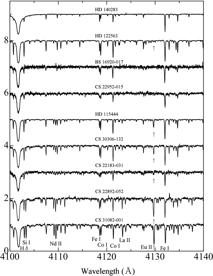
Figure 2: The same as Figure 1, but for the spectral range 4100–4140Å. This region includes lines of H$\delta$ (from which one ascertain that the effective temperatures of these stars are quite similar to one another) and the Eu II 4129 Å line; detections are indicated with a vertical arrow.

References

- Allende Prieto et al. (2000) Allende Prieto, C., Rebolo, R.,Garca Lpez, R, Serra-Ricart, M., Beers, T. C., Rossi, S., Bonifacio, P., Molaro, P. 2000, AJ, 120, 1516
- Aoki et al. (2002) Aoki, W., Norris, J. E., Ryan, S. G., Beers, T. C., Ando, H., & Tsangarides, S. 2002, ApJ, 580, 1149
- Beers, Preston, & Shectman (1985) Beers, T. C., Preston, G. W., & Shectman, S. A. 1985, AJ, 90, 2089
- Beers, Preston, & Shectman (1992) Beers, T. C., Preston, G. W., & Shectman, S. A. 1992, AJ, 103, 1987
- Beers (1999) Beers, T.C. 1999, Ap&SS 265, 547
- Bond (1980) Bond, H. E. 1980, ApJS, 44, 517
- Bonifacio, Monai, & Beers (2000) Bonifacio, P., Monai, S., & Beers, T. C. 2000, AJ, 120, 2065
- Burris et al. (2000) Burris, D. L., Pilachowski, C. A., Armandroff, T. E., Sneden, C., Cowan, J. J., & Roe, H 2000, ApJ, 544, 302
- Carretta et al. (2002) Carretta, E., Gratton, R. G., Cohen, J. G., Beers, T. C., & Christlieb, N. 2002, AJ, 124, 481
- Carney et al. (2003) Carney, B.W., Latham, D.W., Stefanik, R.P., Laird, J.B., & Morse, J.A. 2003, AJ, 125, 293
- Cayrel et al. (2001) Cayrel, R., et al. 2001, Nature, 409, 691
- Cayrel et al. (2004) Cayrel, R., et al. 2004, A&A, in press
- Christlieb (2003) Christlieb, N. 2003, Rev. Mod. Astron. 16, 191 (astro-ph/0308016)
- Christlieb & Beers (2000) Christlieb, N., & Beers, T.C. 2000, Subaru HDS Workshop on stars and galaxies: Decipherment of cosmic history with spectroscopy, NAOJ, Tokyo
- Christlieb et al. (2001) Christlieb, N., Wisotzki, L., Reimers, D., Homeier, D., Koester, D., & Heber, U. 2001, A&A, 366, 898
- Christlieb et al. (2002) Christlieb, N., et al. 2002, Nature, 419, 904
- Cowan et al. (2002) Cowan, J. J., et al. 2002, ApJ, 572, 861
- Den Hartog et al. (2003) Den Hartog, E. A., Lawler, J. E., Sneden, C. & Cowan, J. J. 2003, ApJS, 148, 543
- Fields, Truran, & Cowan (2002) Fields, B. D., Truran, J. W., Cowan, J. J. 2002, ApJ, 575, 845
- Giridhar et al. (2001) Giridhar, S., Lambert, D. L., Gonzales, G., & Pandey, G. 2001, PASP, 113, 519
- Gallino et al. (1998) Gallino, R., Arlandini, C., Busso, M., Lugaro, M., Travaglio, C., Straniero, O., Chieffi, A., & Limongi, M. 1998, ApJ, 497, 388
- Hill et al. (2002) Hill, V., et al. 2002, A&A, 387, 560
- Honda et al. (2003) Honda, S., Aoki, W., Kajino, T., Ando, H., Beers, T. C., Izumiura, H., Sadakane, K., & Takada-Hidai, M. 2003, ApJ, submitted
- Ishimaru & Wanajo (1999) Ishimaru, Y., & Wanajo, S. 1999, ApJ, 511, L33
- Johnson & Bolte (2001) Johnson, J. A., & Bolte, M. 2001, ApJ, 554, 888
- Kurucz et al. (1993) Kurucz, R. L., & Bell, B 1995, Kurucz CD-ROM,No.23 (Harvard-Smithonian Center for Astrophysics)
- Lawler, Bonvallet, & Sneden (2001a) Lawler, J. E., Bonvallet, G., & Sneden, C. 2001a, ApJ, 556, 452
- Lawler et al. (2001b) Lawler, J. E., Wickliffe, M. E., Den Hartog, E. A., & Sneden, C. 2001b, ApJ, 563, 1075
- Lawler et al. (2001c) Lawler, J. E., Wickliffe, M. E., Cowley, C. R., & Sneden, C. 2001c, ApJS, 137, 341
- Lucatello et al. (2003) Lucatello, S., Gratton, R., Cohen, J. G., Beers, T. C., Christlieb, N., Carretta, E., Ramírez, S. 2003 AJ, 125, 875
- McWilliam et al. (1995a) McWilliam, A., Preston, G. W., Sneden, C., & Shectman, S. 1995a, AJ, 109, 2736
- McWilliam et al. (1995b) McWilliam, A., Preston, G. W., Sneden, C., & Searle, L. 1995b, AJ, 109, 2757
- McWilliam (1998) McWilliam, A 1998, AJ, 115, 1640
- Noguchi et al. (2002) Noguchi, K., et al. 2002, PASJ 54, 855
- Norris, Bessell, & Pickles (1985) Norris, J. E., Bessell, M. S., & Pickles, A. J. 1985, ApJS, 58, 463
- Norris et al. (1996) Norris, J. E., Ryan, S. G., & Beers, T. C. 1996, ApJS, 107, 391
- Norris et al. (1997) Norris, J. E., Ryan, S. G., & Beers, T. C. 1997, ApJL, 489, 169
- Norris et al. (2001) Norris, J. E., Ryan, S. G., & Beers, T. C. 2001, ApJ, 561, 1034
- Preston & Sneden (2001) Preston, G. W., & Sneden, C. 2001, AJ, 122, 1545
- Qian & Wasserburg (2001) Qian, Y-Z. & Wasserburg, G. J. 2001, ApJ, 552, L55
- Qian & Wasserburg (2002) Qian, Y-Z. & Wasserburg, G. J. 2002, ApJ, 567, 515
- Rossi et al. (1999) Rossi, S., Beers, T. C., Sneden, C. 1999, in ASP Conf. Ser. 165, The Third Stromlo Symp., The Galactic Halo, ed. B. K. Gibson, T. S. Axelrod, M. E. Putman (San Francisco: ASP), 268
- Ryan et al. (1996) Ryan, S. G., Norris, J. E., & Beers, T. C. 1996, ApJ, 471, 254
- Schatz et al. (2002) Schatz, H., Toenjes, R., Pfeiffer, B., Beers, T. C., Cowan, J. J., Hill, V., & Kratz, K.-L. 2002, ApJ, 579, 626
- Sneden et al. (1996) Sneden, C., McWilliam, A., Preston, G. W., Cowan, J. J., Burris, D. L., & Armosky, B. J. 1996, ApJ, 467, 819
- Sneden et al. (2000) Sneden, C., Cowan, J. J., Ivans, I. I., Fuller, G. M., Burles, S., Beers, T. C. & Lawler, J. E. 2000, ApJL, 533, 139
- Sneden & Cowan (2003) Sneden, C., & Cowan, J. J. 2003, Science, 299, 70
- Sneden et al. (2003) Sneden, C., et al. 2003, ApJ, 591, 936
- Truran et al. (2002) Truran, J. W., Cowan, J. J., Pilachowski, C. A., & Sneden, C. PASP, 114, 1293
- Van Eck et al. (2001) Van Eck, S., Goriely, S., Jorissen, A., Plez, B. 2001, Nature, 412, 793
- Wanajo et al. (2002) Wanajo, S., Itoh, N., Ishimaru, Y., Nozawa, S. & Beers, T.C. 2002, ApJ, 577, 853
- Wanajo et al. (2003) Wanajo, S., Tamamura, M., Itoh, N., Nomoto, K., Ishimaru, Beers, T.C., Nozawa, S. 2003, ApJ, 593, 968
- Westin et al. (2000) Westin, J., Sneden, C., Gustafsson, B., & Cowan, J. J. 2000, ApJ, 530, 783