Convergence and scatter of cluster density profiles

Abstract

We present new results from a series of $\Lambda$CDM simulations of cluster mass halos resolved with high force and mass resolution. These results are compared with recently published simulations from groups using various codes including PKDGRAV, ART, TPM, GRAPE and GADGET. Careful resolution tests show that with 25 million particles within the high resolution region we can resolve to about 0.3% of the virial radius and that convergence in radius is proportional to the mean interparticle separation. The density profiles of 26 high resolution clusters obtained with the different codes and from different initial conditions agree very well. The average logarithmic slope at one percent of the virial radius is $\gamma=1.26$ with a scatter of $\pm 0.17$. Over the entire resolved regions the density profiles are well fitted by a smooth function that asymptotes to a central cusp $\rho\propto r^{-\gamma}$, where we find $\gamma=1.16\pm 0.14$ from the mean of the fits to our six highest resolution clusters.

1 Introduction

A highly motivated and well defined problem in computational astrophysics is to compute the non-linear structure of dark matter halos. This is especially timely given the abundance of new high resolution data that probe the central structure of galaxies (e.g. de Blok et al. 2001a; de Blok, McGaugh & Rubin 2001b; McGaugh, Rubin & de Blok 2001; Swaters et al. 2003; de Blok & Bosma 2002; Gentile et al. 2004) and clusters (e.g. Sand et al. 2004). Furthermore, a standard cosmological paradigm has been defined that gives a well defined framework within which to perform numerical calculations of structure formation (e.g. Spergel et al. 2003). This subject has developed rapidly over the past few years, building upon the pioneering results obtained in the early 1990’s by Dubinski & Carlberg (1991) and Warren et. al (1992). More recently, the systematic study of many halos at a low resolution led to the proposal that the profile of an ‘average’ cold dark matter halo in dynamical equilibrium could be fit by an universal two parameter function (Navarro, Frenk & White, 1996), with a slope of that asymptotically approaches $-1$ as $r\to 0$. At the same time, the study of a few halos at high resolution questioned these results (Fukushige & Makino 1997; Moore et al. 1998; Moore et al. 1999; Jing & Suto 2000; Ghigna et al. 2000). These latter authors claimed that of the order a million particles within the virialised region where necessary to resolve the halo structure to 1% and the slopes at that radius could be significantly steeper. Just within the last few months, we have seen several groups publish reasonably large samples of halos simulated with the necessary resolution that we can finally determine the scatter in the density profiles across a range of mass scales (Fukushige, Kawai & Makino 2004; Tasitsiomi et al. 2004; Wambsganss, Bode & Ostriker 2004; Hayashi et al. 2003; Navarro et al. 2003; Reed et. al 2003).

Much of the recent controversy in the literature has been due to limited statistics and the lack of agreement over what is a reliable radius to trust a given simulation with a given set of parameters. Several studies have attempted to address this issue (Moore et al. 1998; Knebe et al. 2000; Klypin et al. 2001; Power et al. 2003; Diemand et al. 2004). Integration and force accuracy can be understood using controlled test simulations. However, discreteness is probably the most important and least understood numerical effect that can influence our numerical results which is exacerbated due to the lack of an analytic solution with which to compare simulations. Our particle sampling of the nearly collisionless fluid we attempt to simulate can lead to energy transfer and mass redistribution, particularly in the central regions that we are often most interested in.

Collisional effects in the final object or in the early hierarchy of objects can be reduced by increasing the number of particles $N$ in a simulation (Diemand et al., 2004). The limitation to the phase space densities that can be resolved due to discreteness in the initial conditions can also be overcome by increasing the resolution (Binney, 2003). As we increase the resolution within a particular non-linear structure, we find that the global properties of the resolved structure is retained, including shape, density profile, substructure mass functions and even the positions of the infalling substructures. This gives us confidence that our $N$-body calculations are not biased by using finite $N$ (, Baertschiger et al.2002). The fact that increasing the resolution allows us to resolve smaller radii is important since the baryons often probe just the central few percent of a dark matter structure - the latest observations of galaxy and clusters probe the mass distribution within one percent of the virial radius, which until recently was unresolved by numerical simulations. Forthcoming experiments, such as VERITAS (Weekes et. al, 2002) and MAGIC (Flix, Martinez & Prada, 2004) will probe the structure of dark matter halos on even smaller scales by attempting to detect gamma-rays from dark matter annihilation within the central hundred parsecs ($\sim 0.1\%R_{virial}$) of the Galactic halo (e.g. Calcaneo-Roldan & Moore 2000). These scales are still below the resolution limit of todays cosmological simulations, the estimates of the dark matter densities in these regions are still based on extrapolations which introduce large uncertainties

A simple estimate of the scaling of $N$ with time shows remarkable progress over and above that predicted by Moore’s law. The first computer simulations used of the order $10^{2}$ particles and force resolution of the order of the half mass radii (Peebles, 1970). Today we can follow up to $10^{8}$ particles with a resolution of $10^{-3}$ of the final structure. The increase in resolution is significantly faster than predicted by Moore’s law since equally impressive gains in performance have been due to advances in software.

We are finally at the stage whereaby the dark matter clustering is understood at a level where the uncertainties are dominated by the influence of the baryonic component. It is therefore a good time to review and compare existing results from different groups together with a set of new simulations that we have carried out that are the state of the art in this subject and represent what is achievable with several months of dedicated supercomputer time. For certain problems, such as predicting the annihilation flux discussed earlier, it would be necessary to significantly increase the resolution. This is not possible with existing resources and new techniques should be explored. We begin by presenting our new simulations in Section 2. Section 3 discusses convergence tests and the asymptotic best fit density profiles. In Section 4 we compare our results with recently published results from four other groups mentioned above.

2 Numerical Experiments

Table 1 gives an overview of the simulations we present in this paper. With up to $25\times 10^{6}$ particles inside the virial radius of a cluster and an effective $10^{5}$ timesteps, they are among the highest resolution $\Lambda$CDM simulations performed so far. They represent a major investment of computing time, the largest run was completed in about $10^{5}$ CPU hours on the zBox supercomputer .

Table 1: Parameters of simulated cluster halos

Run	$z_{i}$	$\epsilon_{0}$	$\epsilon_{\rm max}$	$N_{\rm vir}$	$M_{\rm vir}$	$r_{\rm vir}$	$Vc_{\rm max}$	$r_{\rm max}$	$r_{\rm resolved}$
		[kpc]	[kpc]		$10^{15}[{\rm M_{\odot}}]$	[kpc]	[km s1]	[kpc]	[kpc]
$A9$	40.27	2.4	24	24’987’606	1.29	2850	1428	1853	9.0
$B9$	40.27	4.8	48	11’400’727	0.59	2166	1120	1321	14.4
$C9$	40.27	2.4	2.4	9’729’082	0.50	2055	1090	904	9.0
$D3h$	29.44	1.8	18	205’061	0.28	1704	944	834	27
$D6h$	36.13	1.8	18	1’756’313	0.31	1743	975	784	13.5
$D6$	36.13	3.6	36	1’776’849	0.31	1749	981	840	13.5
$D9$	40.27	2.4	24	6’046’638	0.31	1752	983	876	9.0
$D9lt$	40.27	2.4	24	6’036’701	0.31	1752	984	841	9.0
$D12$	43.31	1.8	18	14’066’458	0.31	1743	958	645	6.8
$E9$	40.27	2.4	24	5’005’907	0.26	1647	891	889	9.0
$F9$	40.27	2.4	24	4’567’075	0.24	1598	897	655	9.0
$F9cm$	40.27	2.4	2.4	4’566’800	0.24	1598	898	655	9.0
$F9ft$	40.27	2.4	99.06	4’593’407	0.24	1601	905	464	9.0

2.1 N-body code and numerical parameters

The simulations have been performed using a new version of PKDGRAV, written by Joachim Stadel and Thomas Quinn (Stadel, 2001). The code was optimised to reduce the computational cost of the very high resolution runs we present in this paper. We tested the new version of the code by rerunning the “Virgo cluster” initial conditions (Moore et al., 1998). We confirmed that density profile, shape of the cluster and the amount of substructure it contains is identical to that obtained with the original code presented in Ghigna et al. (1998).

Individual time steps are chosen for each particle proportional to the square root of the softening length over the acceleration, $\Delta t_{i}=\eta\sqrt{\epsilon/a_{i}}$. We use $\eta=0.2$ for most runs, only in run $D9lt$ we used larger timesteps $\eta=0.3$ for comparison. The node-opening angle is set to $\theta=0.55$ initially, and after $z=2$ to $\theta=0.7$. This allows higher force accuracy when the mass distribution is nearly smooth and the relative force errors can be large in the treecode. Cell moments are expanded to fourth order in PKDGRAV, other treecodes typically use just second or first order expansion. The code uses a spline softening length $\epsilon$, forces are completely Newtonian at $2\epsilon$. In Table 1 $\epsilon_{0}$ is the softening length at $z=0$, $\epsilon_{max}$ is the maximal softening in comoving coordinates. In most runs the softening is constant in physical coordinates from $z=9$ to the present and is constant in comoving coordinates before, i.e. $\epsilon_{\rm max}=10\epsilon_{0}$. In runs $C9$ and $F9cm$ the softening is constant in comoving coordinates for the entire run, in run $F9ft$ the softening has a constant physical length for the entire run.

2.2 Initial conditions and cosmological parameters

We adopt a $\Lambda$CDM cosmological model with parameters from the first year WMAP results: $\Omega_{\Lambda}=0.732$, $\Omega_{m}=0.268$, $\sigma_{8}=0.9$, $h=0.71$, (Spergel et al., 2003). The initial conditions are generated with the GRAFIC2 package (Bertschinger, 2001). The starting redshifts $z_{i}$ are set to the time when the standard deviation of the density fluctuations in the refined region reaches $0.2$.

First we run a parent simulation: a $300^{3}$ particle cubic grid with a comoving cube size of $300$ Mpc (particle mass $m_{\rm p}=3.7\times 10^{10}{\rm M_{\odot}}$, force resolution $\epsilon_{0}=100kpc$, $\epsilon_{\rm max}=1Mpc$). Then we use the friends-of-friends (FoF) algorithm (Davis et al., 1985) with a linking length of $0.164$ mean interparticle separations to identify clusters. We found 39 objects with virial masses above $2.3\times 10^{14}{\rm M_{\odot}}$. We selected six of these clusters for resimulation, discarding objects close to the periodic boundaries and objects that show clear signs of recent major mergers at $z=0$. We label the six cluster with letters $A$ to $F$ according to their mass. It turned out that two of the clusters selected in this way (runs $A$ and $C$) have ongoing major mergers at $z=0$ (i.e. two clearly distinguishable central cores), which is not evident from the parent simulation due to lack of resolution. These clusters were evolved slightly into the future to obtain a sample of six ’relaxed’ clusters.

For re-simulation we mark and trace back the particles within a cluster’s virial radius to the initial conditions. All particles which lie within a $4$ Mpc (comoving) thick region surrounding the marked particles in the initial conditions are also added to the refinement region. This ensures that there is no pollution of heavier particles within the virial radius of the resimulated cluster. Typically one third or one quarter of the refinement particles ends up within the virial radius. To reduce the mass differences at the border of the refinement region we define a $5$ Mpc thick ’buffer region’ around the high resolution region, there an intermediate refinement factor of 3 or 4 in length is used. The final refinement factors are $6$, $9$ and $12$ in length, i.e., $216$, $729$ and $1728$ in mass, so that the mass resolution is $m_{\rm p}=2.14\times 10^{7}{\rm M_{\odot}}$ in the highest resolution run. We label each run with a letter indicating the object and number that gives the refinement factor in length. To reduce the mass differences at the border of the refinement region we define a $5$ Mpc thick ’buffer region’ around the high resolution region, there an intermediate refinement factor of 3 or 4 in length is used.

2.3 Measuring density profiles

We define the virial radius $r_{\rm vir}$ such that the mean density within $r_{\rm vir}$ is $178\Omega_{M}^{0.45}\rho_{\rm crit}=98.4\rho_{\rm crit}$ for the adopted model (Eke, Cole & Frenk, 1996). We use 30 spherical bins of equal logarithmic width, centered on the densest region of each cluster using TIPSY . We confirmed that using triaxial bins adapted to the shape of the isodensity surfaces (at some given radius, we tried $0.1$, $0.5$ and $1r_{\rm vir}$) does not change the form of the density profile, in agreement with Jing & Suto (2002). For simplicity and easier comparison to other results we will present only profiles obtained using spherical bins. Data points are plotted at the arithmetic mean of the corresponding bin boundaries; the first bin ends at $1.5$ kpc, the last bin at the virial radius.

3 $\Lambda$CDM Cluster Profiles

3.1 Profile Convergence Tests

Numerical convergence tests show that with sufficient timesteps, force accuracy and force resolution the radius a CDM simulation can resolve is limited by the mass resolution (Moore et al. 1998; Ghigna et al. 2000; Knebe et al. 2000; Klypin et al. 2001; Power et al. 2003; Hayashi et al. 2003; Fukushige et al. 2004; Reed et. al 2003). These tests compare different mass resolution simulations of the same object to determine the resolved radius. The resulting radii scale with $N^{-0.45}$ according to Power et al. (2003), Hayashi et al. (2003) and Fukushige et al. (2004), but only with $N^{-1/3}$ in the tests in Moore et al. (1998),Ghigna et al. (2000) and Reed et. al (2003).

Figure 1: Numerical convergence tests for the cluster profiles: Panel (a): Density profiles of cluster $D$ resolved with $N_{\rm vir}=205k,1.8M,6M$ and $14M$ particles. Panel (b): Logarithmic slope for the profiles from (a). Panel (c): Density profiles of cluster $F$ simulated with different numerical parameters: $F9ft$ used 4096 fixed timesteps and constant $\epsilon$ in physical coordinates as in Fukushige et al. (2004). $F9cm$ and $F9$ used adaptive timesteps $0.2\sqrt{\epsilon(z)/a}$ with comoving softening in $F9$ and mixed comoving/physical softening in $F9$ ($\epsilon_{\rm max}=10\epsilon_{0}$). Panel (d): Logarithmic slope for the profiles from (c).

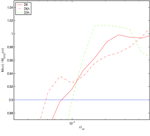
Figure 2: Ratios of the mass enclosed in low resolution runs to mass enclosed in the high resolution run $D12$. By comparing runs with equal softening (smaller than one third of the convergence scale) like $D3h$ and $D6h$ one finds that the resolved radii scale like $r\propto N^{-1/3}$. A larger softening (see run $D6$) can increase the converged scales and change this scaling.

3.1.1 Mass resolution

The finite mass resolution of N body simulations always leads to two body relaxation effects, i.e. heat is transported into the cold halo cores and they expand. It is not obvious that better mass resolution reduces the effects of two body relaxation, since in hierarchical models the first resolved objects always contain just a few particles and with higher resolution these first objects form earlier, i.e. they are denser and more affected by relaxation effects (Moore et al. 2001; Binney & Knebe 2002). Estimates of relaxation based on following the local phase-space density in simulations show that the amount of relaxation can be reduced with better mass resolution, but the average degree of relaxation scales roughly like $N^{-0.3}$ much slower than $N^{-1}$ expected from the relaxation time of the final structure (Diemand et al., 2004). This confirms the validity of performing convergence tests in $N$, but one has to bear in mind that convergence can be quite slow.

Table 2: Convergence radii measured by comparing with run $D12$. The numbers in the run labels are $\propto N^{1/3}$, at fixed force resolution we get $r\propto N^{-1/3}$ (bold values). Question marks indicate that a run with much better mass resolution than $D12$ would be needed to measure this convergence radii reliably. Stars indicate estimated radii assuming a convergence rate of $r\propto N^{-1/3}$.

Run	$\epsilon_{0}$	$N_{\rm vir}$	$r_{\rm 10\%vc}$	$r_{\rm 10\%M}$	$r_{\rm 10\%\rho}$
	[kpc]		[kpc]	[kpc]	[kpc]
$D3h$	1.8	205’061	17.2	21.9	9.5
$D6h$	1.8	1’756’313	8.4	10.7	4.6
$D6$	3.6	1’776’849	8.4	17.3	12.1
$D9$	2.4	6’046’638	3.2 ?	5.2 ?	2.2 ?
$D9lt$	2.4	6’036’701	5.2 ?	6.6 ?	2.8 ?
$D9$	2.4	6’046’638	5.7 *	7.3 *	3.2 *
$D12$	1.8	14’066’458	4.2 *	5.3 *	2.4 *

We checked a series of resimulations of the same cluster (D) for convergence in circular velocity, mass enclosed and density. Outside of the converged radii the values must be within 10% of the reference run D12. Table 2 shows the measured converged radii.

1. Convergence is slow, roughly $\propto N^{-1/3}$. Therefore a high resolution reference run should have at least 8 times as many particles. Between run D9 and D12 the factor is only 2.37. Using D12 to determine the converged radii of D9 gives radii that are about a factor two too small (Table 2). Fukushige et al. (2004) compare runs with $N_{\rm vir}=14\times 10^{6}$ and $N_{\rm vir}=29\times 10^{6}$. At radii where both runs have similar densities it is still not clear if the simulations have converged, even higher resolution studies are needed to demonstrate this.

2. If one sets the force resolution to one half of expected resolved radius, then it is not surprising to measure a resolved radius close to the expected value. With this method one can demonstrate almost arbitrary convergence criteria, as long as they overestimate $r_{conv}$. Therefore convergence tests in $N$ should be performed with small softenings (high force resolution). Runs D3h, D6h and D12 all have $\epsilon_{0}=1.8$ kpc, their converged radii scale like the mean interparticle separation $N^{-1/3}$. In run D6 $\epsilon_{0}=3.2$ kpc is close to the ’optimal value’ from Power et al. (2003), and the converged radii are larger than in D6h (see Figure 2).

3. Different small scale noise in the initial conditions leads to different formation histories. Therefore the shape and the density profile can differ even at radii were all runs have converged. For example between r=10 kpc and 320 kpc the densities in run D9 are about 7% higher than in run D12. Therefore the densities in D9 are within 10% from those of D12 quite early. If one rescales $\rho$ in this range $r_{\rm 10\%\rho}$ of D9 grows from 2.2 kpc to 4.6 kpc.

Extrapolating $r_{\rm conv}\propto N^{-1/3}$ to our highest resolution runs gives the values on the last two lines of Table 2. Note that this is just an extrapolation, it is not clear that this scaling is valid down to this level, only larger simulations could verify this. To be conservative we assume the limit due to mass resolution to be $9$ kpc for the ’9-series’ of runs, and $6.8$ kpc for run D12. The force resolution sets another limit at about $3\epsilon_{0}$ (Moore et al. 1998,Ghigna et al. 2000). We give the larger of the two limits as the trusted radius in Table 1.

3.1.2 Force and time resolution

Finite timesteps and force resolution also sets a limiting radius/density that a run can resolve. We use multistepping, individual timesteps for the particles that are obtained by dividing the main timestep (usually $t_{0}/200$) by two until it is smaller than $\eta\sqrt{\epsilon(z)/a}$, where $a$ is the local acceleration. Our standard choice is $\eta=0.2$ and $\epsilon(z=0)$ between $0.001r_{\rm vir}$ and $0.0022r_{\rm vir}$, which is chosen to be less than one third of the resolution limit expected from the finite mass resolution. $\epsilon$ is constant in physical length units since $z=9$ and comoving before that epoch. Here we argue that the resolution limit imposed by this choice of multistepping lie well below the scale affected by finite mass resolution.

In run $D9lt$ the number of timesteps was reduced by using $\eta=0.3$, at equal force resolution as in $D9$. Run $F9cm$ had a constant comoving softening during the entire simulation, in run $F9ft$ the softening is physical and the timesteps are fixed $\Delta t=t_{0}/4096$ and equal for all particles (i.e. the same numerical parameters as in Fukushige et al. (2004)). The density profiles are very similar (Figure 1, Panel c), there is no significant difference above the mass resolution scale of $9$ kpc. There is a small difference in the inner profile of $F9$ compared to $F9ft$ and $F9cm$, at large $z$ this run has larger $\epsilon$ and therefore larger timesteps than $F9cm$. So it is possible that runs with our standard parameters have slightly shallower density profiles at the resolution limit than runs with entirely comoving softening, or runs with a sufficiently large number of fixed timesteps. However run $F9cm$ takes twice as much CPU time as run $F9$ and run $F9ft$ three times more, therefore we accept this compromise.

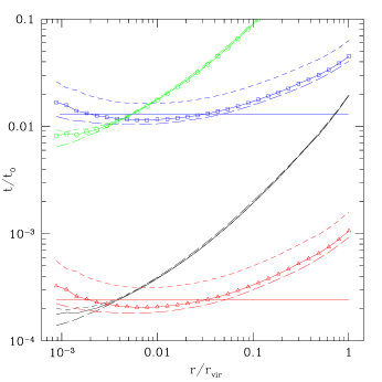
Figure 3: The triangles show the timestep criterium $\eta\sqrt{\epsilon(z)/a}$ as a function of radius for run $D9$ at $z=0$. The dashed line is for run $D9lt$, which has $\eta=0.3$, and the long dashed line for run $D12$. The open squares give $15(\Delta t/t_{0})^{5/6}t_{\rm circ}(r_{vir})$ form Power et al. (2003), the circles are the circular orbit timescale $2\pi r/v_{\rm circ}(r)$. Lines without symbols show $t_{\rm dyn}/15=1/(\sqrt{G\rho(<r)}15)$. The two horizontal lines are the timesteps and $15(\Delta t/t_{0})^{5/6}t_{\rm circ}(r_{vir})$ for run $F9ft$.

Figure 3 shows the timestep criterion $\eta\sqrt{\epsilon(z)/a}$ as a function of radius at $z=0$ for runs $D9$ (triangles, solid line), $D9lt$ (dashed) $D12$ (long dashed) and for $F9ft$ (horizontal line). Particles near the cluster centre must take timesteps below $2\times 10^{-4}t_{0}$, i.e. their timesteps are $t_{0}/200\times 2^{-5}=t_{0}/6400$. According to Power et al. (2003) the resolution limit due to finite timesteps $t_{\rm ts}$ is where the circular velocity (circles) equals $15(\Delta t/t_{0})^{5/6}t_{\rm circ}(r_{vir})$ (open squares). This radius is indeed close to that where the circular velocities and densities start to differ, however for run $D9lt$ this estimate is even a bit too conservative, since the density (and also $v_{\rm circ}$) profiles of $D9lt$ and $D9$ agree down to at least $0.005r_{\rm vir}$. This suggest that about $15$ timesteps per local dynamical time are sufficient for the simulations presented here. Note that this is probably not a general condition for all cosmological simulations: Other codes seem to require different convergence conditions than those we present in this paper. For example, Fukushige et al. (2004) found that their runs converge down to $0.003r_{\rm vir}$ even with only $2048$ fixed timesteps, which corresponds to only eight timesteps per dynamical time at this radius.

3.2 Density Profiles

In this section we present the profiles of the six high resolution runs: $A9$,$B9$,$C9$,$D12$,$E9$,$F9cm$. The output at $z=0$ was used, except for clusters $A9$ and $C9$ which had a recent major merger and the core of the infalling cluster is at about $0.02r_{\rm vir}$ in $A9$ and at $0.1r_{\rm vir}$ in $C9$. These cores spiral in due to dynamical friction and in the ’near’ future both clusters have a regular, ’relaxed’ central region again. Therefore we use outputs at $z=-0.137$ ($+2.1$ Gyr) for run $A9$ and $z=-0.167$ ($+2.6$ Gyr) for $C9$.

3.3 Two parameter fits

Figure 4 shows the density profiles of the six different clusters. We also show best fits to functions previously proposed in the literature that have asymptotic central slopes of -1 (Navarro, Frenk & White 1996;NFW) and -1.5 (Moore et al. 1999;M99). The fits are carried out over the resolved region by minimising the mean square of the relative density differences. These two profiles have two free parameters, namely the scale radius $r_{s}$ and the density at this radius $\rho_{s}=\rho(r_{s})$. The scale radii $r_{s}$ of these best fits give the concentrations $c=r_{\rm vir}/r_{s}$ listed in Table 3. The residuals are plotted in the top and bottom panels of Figure 4 and the rms of the residual are given in Table 3 as $\Delta_{\rm NFW}$ and $\Delta_{\rm M99}$. The residuals are quite large and show that neither profile is a good fit to all the simulations which lie somewhere in between these two extremes.

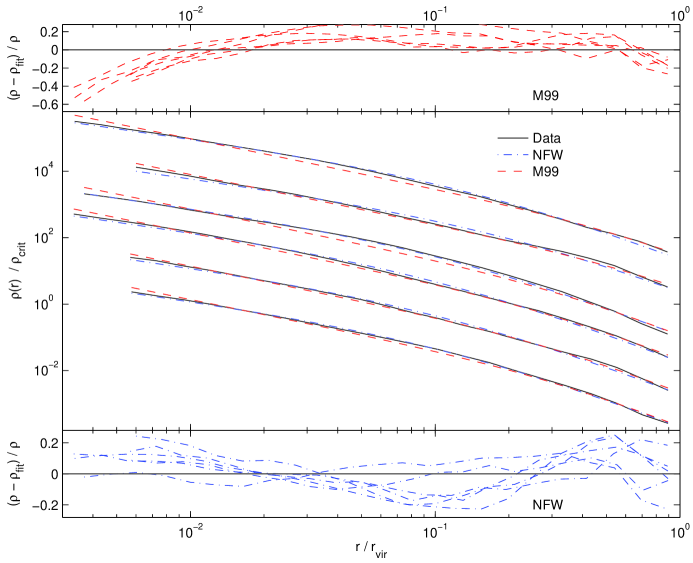
Figure 4: Density profiles of the six clusters in our sample, clusters $B$ to $F$ are shifted downwards for clarity. Clusters are ordered by mass form top to bottom. Profiles of cluster $A$ and $C$ are shown at redshifts $-0.14$ and $-0.17$, i.e. when they have reached a ’relaxed’ state with one well defined centre. Best fit NFW and M99 profiles and residual are shown, obtained by minimising the squares of the relative density differences.

Table 3: Density profile parameters. $\Delta$ is the root mean square of $(\rho-\rho_{\rm fit})/\rho$ for the four fitting functions used.

Run	$c_{\rm NFW}$	$\Delta_{\rm NFW}$	$c_{\rm M99}$	$\Delta_{\rm M99}$	$\gamma_{\rm G}$	$c_{\rm G}$	$\Delta_{\rm G}$	$\alpha_{\rm N}$	$c_{\rm N}$	$\Delta_{\rm N}$
$A9$	5.7	0.10	1.7	0.21	1.16	3.9	0.057	0.167	4.2	0.033
$B9$	4.2	0.16	1.5	0.13	1.29	2.1	0.083	0.141	2.6	0.093
$C9$	7.6	0.09	3.0	0.26	0.92	8.7	0.081	0.247	7.2	0.068
$D3h$	7.4	0.17	3.9	0.13	1.42	4.0	0.103	0.175	7.3	0.101
$D6h$	7.9	0.11	3.8	0.13	1.17	4.6	0.089	0.206	7.2	0.081
$D6$	7.9	0.12	3.8	0.16	1.25	5.4	0.101	0.193	7.2	0.097
$D9$	8.8	0.12	3.9	0.12	1.21	6.2	0.096	0.190	7.8	0.087
$D9lt$	8.7	0.12	3.8	0.12	1.20	6.2	0.098	0.191	7.7	0.087
$D12$	8.4	0.12	3.1	0.14	1.25	4.5	0.066	0.174	6.9	0.051
$E9$	7.4	0.12	3.0	0.10	1.25	4.5	0.072	0.176	6.2	0.069
$F9$	6.9	0.06	3.0	0.14	1.02	6.7	0.054	0.224	6.5	0.048
$F9cm$	7.3	0.06	3.1	0.14	1.10	6.2	0.055	0.212	6.6	0.057
$F9ft$	7.2	0.05	3.1	0.16	1.05	6.6	0.043	0.218	6.5	0.045

3.4 Three parameter fits

Navarro et al. (2003) argue the large residuals of NFW and M99 fits are evidence against any constant asymptotic central slope and propose a profile which curves smoothly over to a constant density at very small radii:

$$\ln(\rho_{\rm N}(r)/\rho_{s})=(-2/\alpha_{\rm N})\left[(r/r_{s})^{\alpha_{\rm N}}-1\right]\,$$ (1)

This function gives a much better fit to the simulations, see the dashed dotted lines in Figure 5, but this should be expected since there is an additional third free parameter $\alpha_{\rm N}$, while the NFW and M99 profiles only have two free parameters. $\alpha_{\rm N}$ determines how fast the profile (1) turns away from an power law near the centre. Navarro et al. (2003) found that $\alpha_{\rm N}$ is independent of halo mass and $\alpha_{\rm N}=0.172\pm 0.032$ for all their simulations, including galaxies and dwarfs. The mean and scatter of our six high resolution clusters is $\alpha_{\rm N}=0.186\pm 0.037$. (Excluding cluster $C9$ yields $\alpha_{\rm N}=0.174\pm 0.025$).

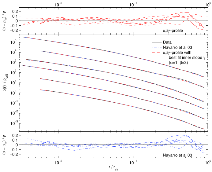
Figure 5: Same as Figure 4, but with fitting functions that have one additional free parameter. The dashed dotted lines show the profile (1) proposed by (Navarro et al., 2003). The dashed lines show a general $\alpha\beta\gamma$-profile (2). We fitted the inner slope $\gamma$ to the data and used fixed values for the outer slope $\beta=3$ and turning parameter $\alpha=1$. $\gamma=1$ corresponds to the NFW profile. The fit parameters and rms of the residuals are given in Table 3.

We also show fits to a general $\alpha\beta\gamma$-profile (Zhao, 1996) ($\rho_{\rm G}$, subscript ’G’ stands for ’general’) that asymptotes to a central cusp $\rho(r)\propto r^{-\gamma}$:

$$\rho_{\rm G}(r)=\frac{\rho_{s}}{(r/r_{s})^{\gamma}(1+(r/r_{s})^{\alpha})^{(\beta-\gamma)/\alpha}}\,.$$ (2)

We fix the outer slope $\beta=3$ and the turnover parameter $\alpha=1$. For comparison the NFW profile has $(\alpha,\beta,\gamma)=(1,3,1)$, the M99 profile has $(\alpha,\beta,\gamma)=(1.5,3,1.5)$. We fit the three parameters $\gamma$, $r_{s}$ and $\rho_{s}$ to the data and find that this cuspy profile also provides a very good fit to the data. The best fit values and rms residual are listed in Table 3 and we find a mean slope of $\gamma=1.16\pm 0.14$.

Using a sharper turnover $\alpha=1.5$ makes the fits slightly worse (the average of $\Delta_{G}$ is about 20 percent larger) and the best fit inner slopes are somewhat steeper $\gamma=1.31\pm 0.11$. We also made some attempts with fitting procedures where $\alpha$ or $\beta$ or both $\alpha$ and $\beta$ are also free parameters. Like Klypin et al. (2001) we found strong degeneracies, i.e. very different combinations of parameter values can fit a typical density profile equally well. Therefore we only present results from the fits with fixed $\alpha$ and $\beta$ parameters in this paper.

The fitting functions (1) and (2) fit the measured density profiles very well over the whole resolved range. Function (1) is even a relatively good approximation below the resolved scale: For example if one is extremely optimistic about $r_{\rm resolved}$ in run $D6$ and uses $r_{\rm resolved}=2.8$ kpc instead of 13.5 kpc one gets $\alpha_{\rm N}=0.0203$, $c_{\rm N}=7.1$ and $\Delta_{\rm N}=0.127$, while the generalised fit is now clearly worse: $\gamma_{\rm G}=0.99$, $c_{\rm G}=3.6$ and $\Delta_{\rm G}=0.216$. Also note that the residuals near $r_{\rm resolved}$ are very small or positive for (1), i.e. the measured density is as large as the fitted value. But at $r_{\rm resolved}$ it is possible that the measured density is slightly too low since in this region the numerical limitations start to play a role. If extrapolation beyond the converged radius is necessary it is not clear which profile is a safer choice. We agree with Navarro et al. (2003) that all simple fitting formula have their drawbacks, that direct comparison with simulations should be attempted whenever possible and that much higher resolution simulations are needed to establish (or exclude) that CDM halos have divergent inner density cusps (as predicted in Binney 2003).

3.5 Maximum inner slope

The results from the last section suggest that profiles with a central cusp in the range $\gamma=1.16\pm 0.14$ provide a good approximation to the inner density profiles of $\Lambda$CDM halos. But Figure 4 in Navarro et al. (2003) seems to exclude our mean value for more than half of their cluster profiles. This is not totally inconsistent, but a hint for a mild discrepancy that we will try to explain: In principle the mass inside the converged radius limits the inner slope: $\gamma_{\rm max}=3(1-\rho(r)/\overline{\rho(,r)})$. This is true if both the density and the cumulative density are correct down to the resolved scale. But up to now the central density of a simulated profile always increased with better numerical resolution, so it is likely that also todays highest resolution simulations underestimate the dark matter density near the centre. This means that cumulative quantities like $v_{\rm circ}(r),\overline{M(<r)}$ and $\overline{\rho(<r)}$ tend to be too low even at radii where the density has converged. The converged radii used in Navarro et al. (2003) are close to the radius where the circular velocity is within 10 percent of a higher resolution run, while the density converges further in at about $0.6r_{\rm conv}$ (Hayashi et al., 2003). If we assume that this is also true for their highest resolution runs then $\overline{\rho(<r)}\propto v_{\rm circ}(r)^{2}$ is up to 20 percent too low, while the error in $\rho(r)$ is much smaller. This raises the values for $\gamma_{\rm max}$ by about $0.2\sim 0.3$ and our mean value $\gamma=1.16$ is not excluded by any of their clusters anymore. If the convergence with mass resolution is not as fast as $r_{\rm conv}\propto N^{-0.45}$ but rather $r_{\rm conv}\propto N^{-1/3}$, see Section 3.1, then the maximum inner slopes could have even larger errors.

4 Comparison with other groups

Recently, several groups have published simulations of dark matter clusters in the concordance cosmological model. These authors kindly supplied their density profiles and we show the comparison here. Fukushige et al. (2004)(’F03’) simulated four $\Lambda$CDM clusters with 7 to 26 million particles using a Treecode and the GRAPE hardware. These authors also used the GRAFIC2 software (Bertschinger, 2001) to generate their initial conditions. Hayashi et al. (2003)(’H03’) and Navarro et al. (2003) presented eight clusters resolved with up to 1.6 million particles within $r_{200}$ simulated with the GADGET code (Springel et al., 2001), the method used to generate the initial conditions is described in Power et al. (2003). Tasitsiomi et al. (2004)(’T03’) simulated six clusters with up to 0.8 million particles within $r_{180}$ using the adaptive refinement tree code ART (Kravtsov et al., 1997) and a technique for setting up multi-mass initial conditions described in Klypin et al. (2001). Wambsganss et al. (2004)(’W03’) present a cosmological simulation without resimulation of refined regions, i.e. constant mass resolution (1024³ particles in a 320 $h^{-1}$Mpc box). The four most massive clusters in this cube are resolved within 0.5 to 0.9 million particles. This simulation was performed with a Tree-Particle-Mesh (TPM) code (Bode & Ostriker, 2003) with a softening of 3.2 $h^{-1}$kpc.

In Figure 6 we show these data along with the new simulations presented in this paper. We plot the density profiles and the logarithmic slopes of the clusters all normalized at the radius such that the circular velocity curve peaks $r_{\rm Vcmax}$ and to $\overline{\rho(<r_{\rm Vcmax})}$. This corresponds to the radius at which $dlog\overline{\rho}/dlogr=-2$. We plot the curves to the “believable” radius stated by each group and down to about 0.01 $r_{\rm vir}$ for W03.

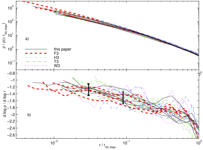
Figure 6: Panel (a): Density profiles of cluster simulated by different groups Normalized to the radius were the circular velocity peaks $r_{\rm Vcmax}$ and to $\overline{\rho(<r_{\rm Vcmax})}$: Six cluster from this paper (solid lines), four from Fukushige et al. (2004) (thick dashed lines), eight from Hayashi et al. (2003) (thin dashed lines), six from Tasitsiomi et al. (2004) (dashed dotted lines)’ four from Wambsganss et al. (2004) (dotted lines). Despite the different codes, parameters and initial conditions used the results are very similar. Panel (b): Logarithmic slope for the profiles from (a). Points with error bars give the averages at 0.03 and 0.09 $r_{\rm Vcmax}$ and a scatter of 0.15 (see Table 4).

The density profiles are reassuringly similar. Furthermore, the scatter is small, the standard deviation of all profiles is roughly $\pm 0.15$ in the logarithmic gradient at small radii ($0.01-0.5r_{\rm Vcmax}$). Table 4 lists the measured slopes at different radii. There is no value at $3\%r_{\rm Vcmax}$ for the cluster from Tasitsiomi et al. (2004) and Wambsganss et al. (2004) because this is below their quoted resolution limit. Most values agree within the scatter, the profiles from Tasitsiomi et al. (2004) are steeper when compared at 0.01 and 0.03 $r_{\rm vir}\equiv r_{98.4}$, but within the scatter at $3\%r_{\rm Vcmax}$. This could be due to different halo selection. The majority of their clusters are not isolated but in close pairs or triplets. In a close pair the density falls slower with radius to 98.4 $\rho_{crit}$, so $r_{\rm vir}\equiv r_{98.4}$ is further out as in a isolated cluster with similar inner profile. Among the samples of isolated clusters (F03; H03; W03 and our clusters) there is a small trend at 0.01 $r_{\rm vir}$ towards steeper slopes with better mass resolution. This could indicate that some numerical flattening of the profiles is still present at 0.01 $r_{\rm vir}$ in the lower resolution clusters.

Table 4: Logarithmic slopes (absolute values) of our six high resolution cluster density profiles. Line (a) gives the averages and scatter. (b)-(c) are average slopes from other groups (see text for details).

	$1\%r_{\rm vir}$	$3\%r_{\rm vir}$	$3\%r_{\rm Vcmax}$	$9\%r_{\rm Vcmax}$
$A9$	1.22	1.36	1.24	1.64
$B9$	1.33	1.43	1.21	1.63
$C9$	1.24	1.21	1.25	1.26
$D12$	1.28	1.54	1.32	1.58
$E9$	1.31	1.44	1.41	1.62
$F9cm$	1.19	1.47	1.22	1.43
a) A-F	1.26$\pm 0.05$	1.41$\pm 0.11$	1.28$\pm 0.08$	1.53$\pm 0.15$
b) F03	1.25$\pm 0.05$	1.52$\pm 0.06$	1.33$\pm 0.15$	1.54$\pm 0.15$
c) H03	1.18$\pm 0.13$	1.38$\pm 0.14$	1.23$\pm 0.17$	1.50$\pm 0.14$
d) T03	1.50$\pm 0.14$	1.79$\pm 0.07$	$-$	1.56$\pm 0.12$
e) W03	1.11$\pm 0.04$	1.41$\pm 0.13$	$-$	1.35$\pm 0.06$
avg.(a-e)	1.26	1.50	$-$	1.49
avg.(a-c)	1.23	1.44	1.28	1.52

5 Summary

We have carried out a series of six very high resolution calculations of the structure of cluster mass objects in a hierarchical universe. The clusters contain up to 25 million particles and have force softening as small as $0.1\%r_{\rm vir}$.

A convergence analysis demonstrates that for our Treecode with our integration scheme, the radius beyond which we can trust the density profiles scale according to the mean interparticle separation. In the best case we reach a resolution of about $0.3\%r_{\rm vir}$.

Neither of the two parameter functions, the NFW and M99 profiles, are very good fits over the whole resolved range in most clusters. One additional free parameter is needed to fit all six clusters: The asymptotically flat profile from Navarro et al. (2003) and an NFW profile with variable inner slope provide much improved fits. The best fit inner slopes are $\gamma=1.16\pm 0.14$. Below the resolved radius the two fitting formulas used are very different. Future simulations with much higher resolution will show which one (if either) of the two is still a good approximation on scales of $0.1\%r_{\rm vir}$ and smaller.

We compare our results with simulations from other groups who used independent codes and initial conditions. We find a good agreement between the cluster density profiles calculated with different algorithms. From $0.03-0.5r_{\rm Vcmax}$ the scatter in the profiles is nearly constant and equal to about 0.17 in logarithmic slope. At one percent of the virial radius (defined such that the mean density within $r_{\rm vir}$ is $178\Omega_{M}^{0.45}\rho_{\rm crit}=98.4\rho_{\rm crit}$) the slope of the density profiles is $1.26\pm 0.16$.

References

- (1) Baertschiger T., Joyce M., Sylos Labini F., 2002, ApJ, 581, L63
- Bertschinger (2001) Bertschinger E., 2001, ApJSS, 137, 1
- Bode & Ostriker (2003) Bode P., Ostriker J. P., 2003, ApJSS, 145, 1
- Binney (2003) Binney J., 2004, MNRAS, 350, 939
- Binney & Knebe (2002) Binney J., Knebe A., 2002, MNRAS, 333, 378
- Calcaneo-Roldan & Moore (2000) Calcáneo-Roldán C., Moore B., 2000, PhRvD, 62, 123005
- Davis et al. (1985) Davis M., Efstathiou G., Frenk C. S., White S.D.M., 1985, ApJ, 292, 371
- de Blok & Bosma (2002) de Blok W. J. G., Bosma A., 2002, A&A, 385, 816
- de Blok et al. (2001a) de Blok W. J. G., McGaugh S. S., Bosma A., Rubin V. C., 2001, ApJ, 552, L23
- de Blok et al. (2001b) de Blok W. J. G., McGaugh S. S., Rubin V. C., 2001, AJ, 122, 2396
- Diemand et al. (2004) Diemand J., Moore B., Stadel J., Kazantzidis S., 2004, MNRAS, 348, 977
- Dubinski & Carlberg (1991) Dubinski J., Carlberg R. G., 1991, ApJ, 378, 496
- Eke et al. (1996) Eke V. R., Cole S., Frenk C. S., 1996, MNRAS, 282, 263
- Flix et al. (2004) Flix J., Martinez M., Prada F., 2004, preprint, , astro-ph/0401511.
- Fukushige & Makino (1997) Fukushige T., Makino J., 1997, ApJ, 477, L9
- Fukushige & Makino (2001) Fukushige T., Makino J., 2001, ApJ, 557, 533
- Fukushige et al. (2004) Fukushige T., Kawai A. and Makino J., 2004, ApJ,. 606, 625
- Gentile et al. (2004) Gentile G., Salucci P., Klein U., Vergani D., Kalberla P.,2004, MNRAS in press, arXiv:astro-ph/0403154.
- Ghigna et al. (1998) Ghigna S., Moore B., Governato F., Lake G., Quinn T., Stadel J.,1998, MNRAS, 300, 146
- Ghigna et al. (2000) Ghigna S., Moore B., Governato F., Lake G., Quinn T., Stadel J., 2000, ApJ, 544, 616
- Hayashi et al. (2003) Hayashi E., Navarro J. F. , Power C., Jenkins A., Frenk C.S., White S. D. M., Springel V., Stadel J., Quinn T., 2003, preprint , astro-ph/0310576.
- Jing & Suto (2000) Jing Y., Suto Y., 2000, ApJ, 529, L69
- Jing & Suto (2002) Jing Y., Suto Y., 2002, ApJ, 574, 538
- Klypin et al. (2001) Klypin A., Kravtsov A. V., Bullock J. S., Primack J. R., 2001, ApJ, 554, 903
- Knebe et al. (2001) Knebe A., Green A., Binney J., 2001, MNRAS, 325, 845
- Knebe et al. (2000) Knebe, A., Kravtsov A. V., Gottlöber S., and Klypin A.A., 2000, MNRAS, 317, 630
- Kravtsov et al. (1997) Kravtsov A. V., Klypin A. A., Khokhlov A. M., 1997, ApJ, 111, 73
- McGaugh, Rubin & de Blok (2001) McGaugh S. S., Rubin V. C., de Blok W. J. G., 2001, AJ, 122, 2381
- Moore et al. (2001) Moore B. 2001, In Martel H. & Wheeler J., eds, AIP Conf. Proc. 586, The dark matter crisis, p.73
- Moore et al. (1998) Moore B., Governato F., Quinn T., Stadel J., Lake G., 1998, ApJ, 499, L5
- Moore et al. (1999) Moore B., Quinn T., Governato F., Stadel J., Lake G., 1999, MNRAS, 310, 1147
- Navarro et al. (1996) Navarro J. F., Frenk C. S., White S. D. M., 1996, ApJ, 462, 563
- Navarro et al. (2003) Navarro J. F., Hayashi E., Power C., Jenkins A., Frenk C. S., White S. M. D., Springel V., Stadel J., Quinn T. R., 2004, MNRAS, 349, 1039
- Peebles (1970) Peebles P. J. E., 1970, AJ, 75, 13
- Power et al. (2003) Power C., Navarro J. F., Jennkins A., Frenk C. S., White S. D. M., 2003, MNRAS, 338, 14
- Reed et. al (2003) Reed D., Governato F., Verde L., Gardner J., Quinn T., Stadel J., Merritt D., Lake G., 2003, preprint, arXiv:astro-ph/0312544.
- Sand et al. (2004) Sand D. J., Treu T., Smith G. P., Ellis R. S., 2004, ApJ, 604, 88
- Spergel et al. (2003) Spergel D. N. et al., 2003, ApJSS, 148, 175
- Springel et al. (2001) Springel V., Yoshida N., White S. D. M., 2001, New Astronomy, 6, 79
- Stadel (2001) Stadel J., 2001, PhD thesis, U. Washington
- Swaters et al. (2003) Swaters R. A., Madore B. F., van den Bosch F. C., Balcells M., 2003, ApJ, 583, 732
- Tasitsiomi et al. (2004) Tasitsiomi A., Kravtsov A. V., Gottlober S., Klypin A. A., 2004, ApJ, 607, 125
- Wambsganss et al. (2004) Wambsganss J., Bode P., Ostriker J. P., 2004, ApJ, 606, L93
- Warren et. al (1992) Warren M. S., Quinn P. J., Salmon J. K., Zurek W. H., 1992, ApJ, 399, 405
- Weekes et. al (2002) Weekes T. C. et al., 2002, Astropart. Phys., 17, 221
- Zhao (1996) Zhao, H. 1996, MNRAS, 278, 488