CHANDRA OBSERVATIONS OF THE “DARK” MOON AND GEOCORONAL SOLAR-WIND CHARGE TRANSFER

Abstract

We have analyzed data from two sets of calibration observations of the Moon made by the Chandra X-Ray Observatory. In addition to obtaining a spectrum of the bright side that shows several distinct fluorescence lines, we also clearly detect time-variable soft X-ray emission, primarily O VII K$\alpha$ and O VIII Ly$\alpha$, when viewing the optically dark side. The apparent dark-side brightness varied by at least an order of magnitude, up to $\sim 2\times 10^{-6}$ phot s^-1 arcmin^-2 cm^-2 between 500 and 900 eV, which is comparable to the typical 3/4-keV-band background emission measured in the ROSAT  All-Sky Survey. The spectrum is also very similar to background spectra recorded by Chandra in low or moderate-brightness regions of the sky. Over a decade ago, ROSAT  also detected soft X-rays from the dark side of the Moon, which were tentatively ascribed to continuum emission from energetic solar wind electrons impacting the lunar surface. The Chandra observations, however, with their better spectral resolution, combined with contemporaneous measurements of solar-wind parameters, strongly favor charge transfer between highly charged solar-wind ions and neutral hydrogen in the Earth’s geocorona as the mechanism for this emission. We present a theoretical model of geocoronal emission and show that predicted spectra and intensities match the Chandra observations very well. We also model the closely related process of heliospheric charge transfer and estimate that the total charge transfer flux observed from Earth amounts to a significant fraction of the soft X-ray background, particularly in the ROSAT  3/4-keV band.

1. INTRODUCTION

As reported by Schmitt et al. (1991), an image of the Moon in soft X-rays (0.1–2 keV) was obtained by the Röntgen Satellite (ROSAT ) using its Position-Sensitive Proportional Counter (PSPC) on 1990 June 29. This striking image showed an X-ray-bright sunlit half-circle on one side, and a much dimmer but not completely dark side outlined by a brighter surrounding diffuse X-ray background. Several origins for the dark-side emission were considered, but the authors’ favored explanation was continuum emission arising from solar wind electrons sweeping around to the unlit side and impacting on the lunar surface, producing thick-target bremsstrahlung. Given the very limited energy resolution of the PSPC, however, emission from multiple lines could not be ruled out.

A significant problem with the bremsstrahlung model was explaining how electrons from the general direction of the Sun could produce events on the opposite side of the Moon, with a spatial distribution which was “consistent with the telescope-vignetted signal of a constant extended source.” An elegant alternative explanation would be a source of X-ray emission between the Earth and the Moon, but at the time, no such source could be envisioned. If this source were also time-variable, it would account for the Long Term Enhancements (LTEs) seen by ROSAT . These occasional increases in the counting rate of the PSPC are vignetted in the same way as sky-background X-rays, indicating an external origin (Snowden et al., 1995). LTEs are distinct from the particle-induced background, and are uncorrelated with the spacecraft’s orientation or position (geomagnetic latitude, etc.), although Freyberg (1994) noted that LTEs appeared to be related, by a then unknown mechanism, to geomagnetic storms and solar wind variations. The final ROSAT  All-Sky Survey (RASS) diffuse background maps (Snowden et al., 1995, 1997) removed the LTEs, so far as possible, by comparing multiple observations of the same part of the sky, but any constant or slowly varying ($\tau\gtrsim 1$ week) emission arising from whatever was causing the LTEs would remain.

A conceptual breakthrough came with the ROSAT  observation of comet Hyakutake (Lisse et al., 1996) and the suggestion by Cravens (1997) that charge transfer (CT) between the solar wind and neutral gas from the comet gave rise to the observed X-ray emission. In solar-wind charge transfer, a highly charged ion in the wind (usually oxygen or carbon) collides with neutral gas (mostly water vapor in the case of comets) and an electron is transferred from the neutral species into an excited energy level of the wind ion, which then decays and emits an X-ray. This hypothesis has been proven by subsequent observations of comets such as C/LINEAR 1999 S4 by Chandra (Lisse et al., 2001) and Hyakutake by EUVE (Krasnopolsky & Mumma, 2001) (see also the review by Cravens (2002)), and is supported by increasingly detailed spectral models (Kharchenko et al., 2003; Kharchenko & Dalgarno, 2000). A more extensive history of the evolution of the solar-wind CT concept can be found in Cravens, Robertson, & Snowden (2001) and Robertson & Cravens (2003a).

Citing the cometary emission model, Cox (1998) pointed out that CT must occur throughout the heliosphere as the solar wind interacts with atomic H and He within the solar system. Freyberg (1998) likewise presented ROSAT  High-Resolution Imager data that provided some evidence for a correlation between increases in the apparent intensity of comet Hyakutake and in the detector background; he further suggested that this could be caused by charge transfer of the solar wind with the Earth’s atmosphere. A rough broad-band quantitative analysis by Cravens (2000) predicted that heliospheric emission, along with CT between the solar wind and neutral H in the Earth’s tenuous outer atmosphere (geocorona), accounts for up to half of the observed soft X-ray background (SXRB). Intriguingly, results from the Wisconsin Soft X-Ray Background sky survey (McCammon & Sanders, 1990) and RASS observations (Snowden et al., 1995) indicate that roughly half of the 1/4-keV background comes from a “local hot plasma.” Cravens, Robertson, & Snowden (2001) also modeled how variations in solar-wind density and speed should affect heliospheric and geocoronal CT emission observed at Earth, and found strong correlations between the measured solar-wind proton flux and temporal variations in the ROSAT  counting rate.

In this paper we present definitive spectral evidence for geocoronal CT X-ray emission, obtained in Chandra observations of the Moon. Data analysis is discussed in §2, and results are presented in §3. As we show in §4, model predictions of geocoronal CT agree very well with the observed Chandra spectra. In §5 we estimate the level of heliospheric CT emission, discuss the overall contribution of CT emission to the SXRB, and assess the observational prospects for improving our understanding of this subtle but ubiquitous souce of X-rays.

2. THE DATA

Table 1Observation Information

			Exposure	Chandra
ObsID	Date	CCDs	(s)	Time
2469	2001 Jul 26	I23, S23	2930	112500070–112503000
2487	2001 Jul 26	I23, S23	2982	112503320–112506302
2488	2001 Jul 26	I23, S23	2747	112507858–112510605
2489	2001 Jul 26	I23, S23	2998	112510900–112513898
2490	2001 Jul 26	I23, S23	2830	112515450–112518280
2493	2001 Jul 26	I23, S23	2993	112518500–112521493
2468	2001 Sep 22	I23, S123	3157	117529483–117532640
3368	2001 Sep 22	I23, S123	2223	117532850–117535073
3370	2001 Sep 22	I23, S123	4772	117536678–117541450
3371	2001 Sep 22	I23, S123	3998	117541880–117545878

Note. — Chandra time 0 corresponds to the beginning of 1998. Observations run from July 26 02:01:10–07:58:13 UT, and September 22 07:04:43–11:37:58 UT.

The Moon was observed with the Chandra Advanced CCD for Imaging Spectroscopy (ACIS) in two series of calibration observations on 2001 July 26 and September 22 totaling 17.5 and 14 ksec, respectively (see Table 1). The intention was to determine the intrinsic ACIS detector background by using the Moon to block all cosmic X-ray emission. Four of the ACIS CCDs were used in July (I2 and I3 from the ACIS-Imaging array, and S2 and S3 from the ACIS-Spectroscopy array), and the S1 chip was added in September. Two of the chips, S1 and S3, are back-illuminated (BI) and have better quantum efficiency at low energies than the front-illuminated (FI) chips, I2, I3, and S2. As can be seen in Fig. 1, however, the BI chips have higher intrinsic background than the FI chips, and also poorer energy resolution. Telemetry limits prevented the operation of more CCDs when using ACIS Very Faint mode, which was desired because of its particle-background rejection utility (Vikhlinin, 2001).

The ACIS detector background was also calibrated in an alternative manner using Event Histogram Mode (EHM; Biller, Plucinsky, & Edgar (2002)). The July Moon and EHM spectra from the S3 ship were compared by Markevitch et al. (2002) and showed good agreement, although there was a noticeable but statistically marginal excess near 600 eV in the Moon data.

The dark-Moon vs EHM comparison strongly supports the assumption that the high-energy particle background inside the detector housing where EHM data are collected is the same as in the focal position. With that in mind, new calibration measurements were made on 2002 September 3 with ACIS operating with its standard imaging setup in a “stowed” position, where it was both shielded from the sky and removed from the radioactive calibration source in its normal off-duty position. (Markevitch, 2002). These data (ObsID 62850, 53 ks) provide the best available calibration of the intrinsic detector background and are used in the analysis that follows.

2.1. Data Preparation

All data were processed to level 1 using Chandra Interactive Analysis of Observations (CIAO) software, Pipeline release 6.3.1, with bad-pixel filtering. Start and stop times for each observation were chosen to exclude spacecraft maneuvers. Apart from the inclusion of CTI corrections (see below) and a more aggressive exclusion of any possibly questionable data, our data processing is essentially the same as that described by Markevitch et al. (2002), who limited their analysis to the July S3 data. Here we use data from all chips during both the July and September observations, and include data from periods of partial dark-Moon coverage by using spatial filtering (see §2.2).

Although ACIS has thinly aluminized filters to limit optical contamination, the sunlit side of the Moon was so bright that an excess bias signal was sometimes produced in the CCDs, particularly in the I2 and I3 chips that imaged that region during July. As described in Markevitch et al. (2002), a bias correction to each event’s pulse height amplitude was calculated by averaging the 16 lowest-signal pixels of the 5$\times$5-pixel Very Faint (VF) mode event island. ObsID 2469 suffered by far the most optical contamination, so that all data from the I2 chip during that observation had to be discarded. The I3 chip also had significant contamination, but it was small enough to be largely corrected. As explained in §2.3, however, I3 data from that observation were also excluded as a precaution. Two other July observations required exclusion of some I2 data because of optical leaks (930 s in ObsID 2490 and 1140 s in Obsid 2493), but in all the remaining data the typical energy correction was no more than a few eV, which is insignificant for our purposes.

To improve the effective energy resolution, we applied standard charge transfer inefficiency (CTI) corrections, as implemented in the CIAO tool acis_process_events, to data from the FI chips. CTI is much less of a problem in the BI chips, S1 and S3, and no corrections were made to those chips’ data. Finally, VF-mode filtering was applied to all the data (Vikhlinin, 2001) to reduce the particle-induced detector background. The “ACIS stowed” background data were treated in the same way, except that no optical-contamination corrections were required.

2.2. Spatial Extractions

Figure 1.— Moon motion across the ACIS chips during July and September observations. Green denotes Moon position at the start of the observation and red at the end. The illuminated portion of the Moon is the crescent on the right. Dark-side gibbous extraction regions provide a 90” buffer along the Moon limb and terminator. S1 and S3 chips are darker because of their higher background.

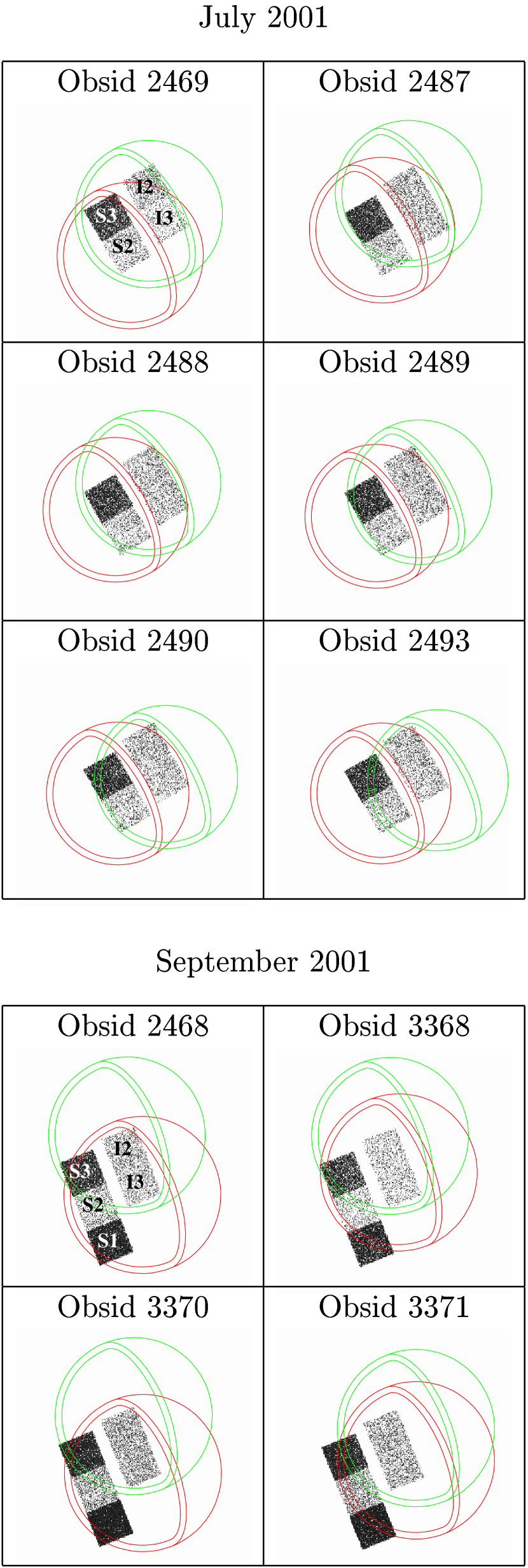
As seen in Fig. 1, Chandra pointed at a fixed location on the sky during each observation as the Moon drifted across the field of view. Using ephemerides for the Moon and Chandra’s orbit, we calculated the apparent position and size of the Moon in 1-minute intervals and extracted data from its dark side, as well as from the bright side and from the unobscured cosmic X-ray background (CXB) within the field of view for comparison. Because the Moon moved by up to 16” per minute, and to avoid X-ray “contamination” of data within each extraction region (particularly spillover of bright-side or CXB photons into the dark side) we used generous buffers of 90” from the terminator and limb for the dark-side extraction, 30” from the terminator and 60” from the limb for bright-side data, and 60” from the limb for the CXB data. Chandra has a very tight point spread function, with an on-axis encircled energy fraction of nearly 99% at 500 eV within 10”; although off-axis imaging is involved here, estimated X-ray contamination is less than $\sim 2$% within our chosen extraction regions.

Data from all ObsIDs were analyzed in several energy bands to look for discrete sources but none were found, and lightcurves for each observation behave as would be expected for uniform emission within each extraction region. Effective exposure times (as if one CCD were fully exposed) were computed for each ObsID/chip/extraction combination by computing extraction areas for each 1-minute interval (accounting for spacecraft dither, which affects area calculations near the chip edges) and summing the area$\times$time products. Results are listed in Table 2.

Table 2Effective Exposure Times Per Chip

	Dark-Side Region						Bright-Side Region
ObsID	I2	I3	S1	S2	S3		I2	I3	S1	S2	S3
2469	0	0	…	2930	2924		0	0	…	0	0
2487	1702	1759	…	2812	2982		722	704	…	0	0
2488	1204	1233	…	2714	2747		979	965	…	0	0
2489	1491	1375	…	2978	2977		984	1062	…	0	0
2490	1071	1306	…	2811	2714		984	1062	…	0	0
2493	1456	1637	…	2862	2572		238	847	…	0	0
Total	6924	7310	…	17107	16916		3503	4560	…	0	0
2468	3157	3150	1026	2534	2958		0	0	1462	177	6
3368	2223	2223	162	1364	2031		0	0	1680	275	0
3370	4772	4770	1281	3479	3611		0	0	2157	439	20
3371	3995	3995	265	1631	1803		0	0	3024	1114	950
Total	14147	14138	2734	9008	10403		0	0	8323	2005	976

Because the detector background is not perfectly uniform across each chip, background data were projected onto the sky and extracted using the same regions as for the dark-Moon data. Exposure-weighted and epoch-appropriate detector response functions (RMFs and ARFs) were then created using standard CIAO threads, including the corrarf routine, which applies the ACISABS model to account for contaminant build-up on ACIS. The detector background rate varies slightly on timescales of months, so we renormalized the background data to match the corresponding observational data in the energy range 9.2–12.2 keV, where the detected signal is entirely from intrinsic background. The required adjustments were only a few percent.

2.3. Spectra

As described by Markevitch et al. (2002), the BI chips, and very rarely the FI chips, often experience “soft” background flares because of their higher sensitivity to low-energy particles. A relatively bright flare was found in ObsID 3370, and 400 seconds of data were removed. Weaker flares are more common and we judged it better to model and subtract their small effects rather than exclude large intervals of data. Soft flares have a consistent spectral shape (a powerlaw with high-energy cutoff) and their intensity at all energies can be determined by integrating the excess signal (above the “stowed” background) in the energy range 2.5–7 keV where the relative excess is most significant. We find that spectra from ObsIDs 2468 and 3368 have minor soft-flare components, and have accounted for them in the results presented later. An essentially negligible soft-flare excess is also seen and accounted for when all the July S3 data are combined.

Figure 2.— Spectrum of the bright side of the Moon, combining I2 and I3 data from all July observations except ObsID 2469, binned by 2 PI channels (29.2 eV). Dotted curve is detector background. Fluorescence K-shell lines from O, Mg, Al, and Si are shifted up by 50 eV from their true values because of residual errors when correcting for detector sensitivity to optical photons (see text). Optical contamination effects likewise cause slight mismatches in energies of intrinsic detector features such as the Au-M complex (2.2 keV), Ni-K (7.5 keV), and Au-L$\alpha$ (9.7 keV). There are $\sim$1300 counts in the O-K line.

Figure 3.— Observed and background-subtracted spectra from the dark side of the Moon, with 2-channel (29.2 eV) binning. In the July S3 data (top four panels), no excess emission is obvious except in ObsID 2469. Features around 1750 eV (Si-K) and 2150 eV (Au-M) are from particle-induced fluorescence of the detector assembly. Bottom four panels show S3 and combined FI spectra from the three September ObsIDs with the strongest emission excesses. Oxygen emission from charge transfer is clearly seen in both spectra, and energy resolution in the FI chips is sufficient that O VIII Ly$\alpha$ is largely resolved from O VII K$\alpha$. High-$n$ O VIII Lyman lines are also apparent in the FI spectrum, along with what is likely Mg XI K$\alpha$ around 1340 eV.

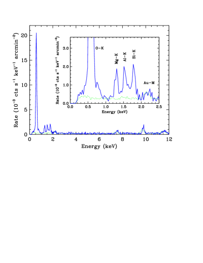
One last complication is the effect of optical contamination on the energy calibration. Although raw energy offsets were removed from the data during the bias-correction process, more subtle effects remained, mostly related to charge transfer inefficiency. Optical-leak events partially fill the charge traps in the CCDs, thus reducing the net CTI. When standard CTI corrections were applied to the data to improve the energy resolution of the FI chips, this overcorrected and pushed energies too high for data affected by the optical leak. The effect varies between and within chips based on optical exposure, but we can place an upper limit on it by examining the bright-Moon data, which are most affected. Fig. 2 shows the spectrum of the combined July bright-Moon data, which come from the I2 and I3 chips. The $K$-shell fluorescence lines of O, Mg, Al, and Si are easily identified, and we find a positive offset of $50\pm 5$ eV from their true values of 525, 1254, 1487, and 1740 eV, respectively. Bright-side data from ObsID 2469 I3 were excluded because they showed an offset of roughly 80 eV, with a distorted shape for the O peak; to be conservative, we excluded the corresponding dark-side data from further consideration as well. As noted before, I2 data from ObsID 2469 were already excluded because of their much larger optical contamination.

Energy offsets in the dark-side and CXB data should be much smaller, particularly for the S chips, which did not image the bright side of the Moon. Judging from the positions of weak fluorescence lines present in the detector background, and the agreement of astrophysical line positions in the FI and S3 spectra with each other and theoretical models (see §4.1), the dark-side energy errors indeed appear to be negligible.

3. RESULTS

3.1. Dark-Side Spectra

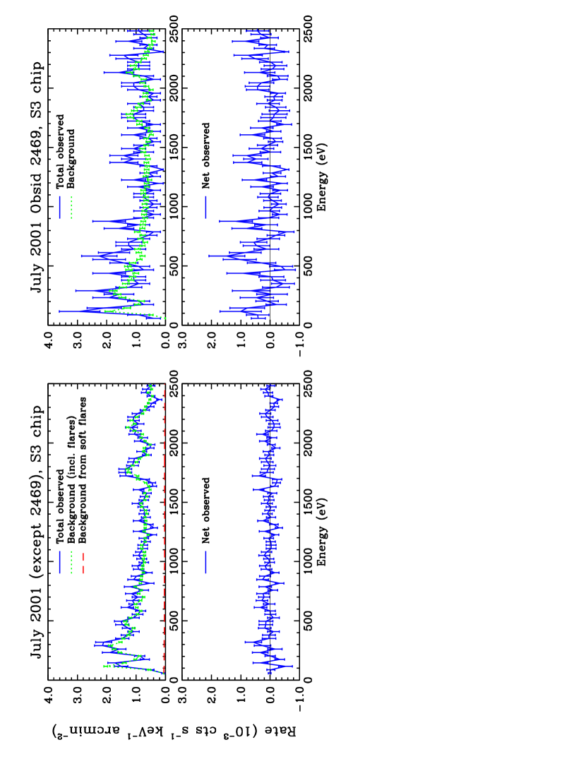
X-ray spectra were created from the event files using CIAO dmextract. Data from the three FI chips (I2, I3, and S2), which have lower QE than the BI chips below 1 keV, were always combined in order to improve statistics. Scaled background spectra, with soft-flare corrections as needed, were created for each observed dark-side spectrum and subtracted to reveal any excess X-ray emission.

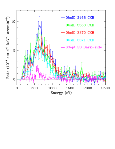
Summing all the July data apart from ObsID 2469 reveals no significant excesses in either the S3 or combined FI spectra (see top half of Fig. 3). The S3 spectrum from ObsID 2469, however, has a noticeable emission feature (more than $3\sigma$) at $\sim 600$ eV. The corresponding FI spectrum for ObsID 2469 has too few counts to be used for corroboration as it includes only data from the S2 chip (because of the optical leaks in I2 and I3).

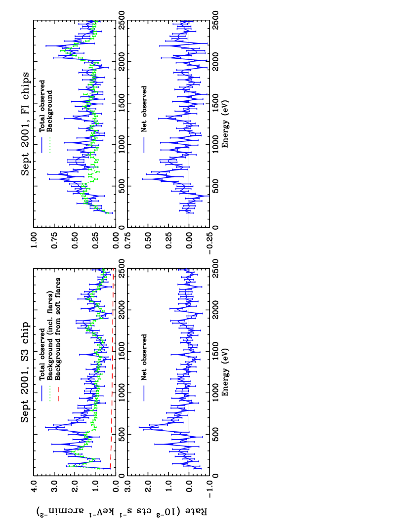
Much stronger evidence for excess emission near 600 eV appears in the September dark-Moon spectra, in all chips (bottom half of Fig. 3). It is immediately obvious that this can not be particle- or photon-induced O fluorescence, which would occur in a single line at 525 eV, nor is it electron-impact continuum as posited by Schmitt et al. (1991).

To assess the significance of any excesses, we selected three energy ranges for statistical study with the a priori assumption that solar-wind charge transfer is the source of the emission (§4). Each range (311–511 eV, 511–711 eV, and 716–886 eV) was chosen to extend $\sim 50$ eV below and above the strongest CT lines expected within each range (§4.1). For comparison, the 886–986 eV band was also studied (in which we might hope to see Ne IX K$\alpha$ at 905–922 eV), along with four 200-eV-wide bands from 1000 to 1800 eV. The most important results are shown in Table 3, with excesses of more than $2.5\sigma$ shown in bold.

Table 3Net Emission Within Selected Energy Bands

			311–511 eV			511–716 eV			716–886 eV			886–986 eV
			Counting	Signif.		Counting	Signif.		Counting	Signif.		Counting	Signif.
Chips	ObsIDs		Rate	($\sigma$)		Rate	($\sigma$)		Rate	($\sigma$)		Rate	($\sigma$)
FIs	2469		$2\pm 19$	0.1		$25\pm 20$	1.2		$6\pm 16$	0.4		$25\pm 16$	1.5
FIs	all July		$-1\pm 6$	-0.2		$3\pm 6$	0.5		$7\pm 5$	1.5		$3\pm 4$	0.7
FIs	2468		$2\pm 12$	0.1		$\mathbf{65\pm 14}$	4.5		$\mathbf{32\pm 12}$	2.8		$-1\pm 7$	-0.1
FIs	3368		$-11\pm 13$	-0.9		$\mathbf{76\pm 18}$	4.2		$22\pm 13$	1.7		$18\pm 11$	1.7
FIs	3370		$-5\pm 9$	-0.5		$12\pm 9$	1.3		$18\pm 9$	2.1		$2\pm 6$	0.3
FIs	3371		$1\pm 11$	0.1		$26\pm 12$	2.2		$22\pm 10$	2.1		$15\pm 8$	1.9
FIs	3 bright		$-2\pm 7$	-0.3		$\mathbf{52\pm 8}$	6.3		$\mathbf{26\pm 7}$	3.9		$10\pm 5$	2.1
S3	2469		$-36\pm 34$	-1.1		$\mathbf{126\pm 39}$	3.2		$29\pm 30$	1.0		$-19\pm 17$	-1.1
S3	quiet July		$30\pm 18$	1.7		$22\pm 15$	1.4		$13\pm 13$	1.0		$6\pm 10$	0.7
S3	all July		$22\pm 16$	1.4		$\mathbf{43\pm 14}$	3.0		$18\pm 12$	1.5		$4\pm 8$	0.4
S3	2468		$51\pm 31$	1.7		$\mathbf{218\pm 33}$	6.6		$27\pm 23$	1.2		$9\pm 16$	0.5
S3	3368		$54\pm 54$	1.0		$\mathbf{256\pm 61}$	4.2		$18\pm 40$	0.4		$11\pm 30$	0.4
S3	3370		$58\pm 37$	1.5		$77\pm 34$	2.3		$-21\pm 24$	-0.9		$-15\pm 17$	-0.9
S3	3371		$26\pm 49$	0.5		$\mathbf{247\pm 60}$	4.1		$\mathbf{214\pm 54}$	4.0		$72\pm 35$	2.0
S3	3 bright		$63\pm 28$	2.2		$\mathbf{228\pm 31}$	7.3		$\mathbf{58\pm 23}$	2.6		$18\pm 16$	1.2

Note. — Rate excesses of more than 2.5$\sigma$ are shown in bold. “FIs” means the I2, I3, and S2 chips in combination.

^a Units of $10^{-6}$ cts s^-1 arcmin^-2.  ^b Chip S2 only; data from I2 and I3 are unusable.  ^c ObsIDs 2469, 2487, 2488, 2489, 2490, and 2493.  ^d The “bright-September” ObsIDs: 2468, 3368, and 3371.  ^e All July ObsIDs except 2469.

Emission in the 511–711 eV range has an excess of more than $4\sigma$ in three of the four S3 spectra from September, and $2.3\sigma$ in the other (ObsID 3370). The same pattern (most significant excess in ObsID 2468, least in ObsID 3370) holds for the combined FI spectra. When spectra from the three ObsIDs showing the largest excesses (2468, 3368, and 3371, henceforth referred to as the “bright-September” ObsIDs) were summed, the feature significance was more than $6\sigma$ in both the S3 and FI spectra (see Table 3). The ratio of net counting rates for S3 and the FI chips ($4.3\pm 0.9$) also matches well with the ratio of those chips’ effective areas in that energy range, consistent with this being an X-ray signal from the sky. Results from the S1 chip were consistent with those from S3, but with lower significance because of the S1’s much shorter dark-Moon exposure times and somewhat higher background; we do not discuss S1 dark-side results further.

The 716–886 eV range, which we expect to contain O VIII Ly$\beta$ and O VIII Ly$\delta$ emission, also showed significant excesses in the S3 and combined FI spectra for the bright-September ObsIDs ($\sim 2.5\sigma$ and $\sim 4\sigma$, respectively) with excesses in individual ObsIDs roughly following the time pattern seen in the 511–711-eV band. The S3 spectrum for ObsID 3371 stands out with a $4\sigma$ excess. The same ObsID also has $2\sigma$ excesses in the 886–986 eV range in both the S3 and FI spectra. This energy range, like the 716–886 eV range, contains CT emission lines (Ne IX K$\alpha$ at 905–922 eV) from an ion which is only abundant when the solar wind is especially highly ionized. As we will discuss in §4.3, there is evidence for such a situation during ObsID 3371.

Above 1000 eV, no significant excesses were seen for any of the ObsID combinations listed in Table 3 with the possible exception of 1200–1400 eV, which had a $2.9\sigma$ excess in the bright-September FI spectrum (and a $1.0\sigma$ excess in the S3 spectrum). Again, 3371 was the individual ObsID recording the largest excesses in the FI ($1.8\sigma$) and S3 ($1.3\sigma$) spectra. Although the evidence is not compelling, we believe that the observed excess probably represents a detection of He-like Mg XI K$\alpha$ ($\sim 1340$ eV).

In the 311–511 eV range where C VI Lyman emission might be detectable, only a $2.2\sigma$ excess appears in the S3 data. Over the full range of O emission (511–886 eV), which is relevant to the discussion in §4, the bright-September S3 and FI spectra both have an excess of $7.4\sigma$, with net rates of $287\pm 39$ and $78\pm 11\times 10^{-6}$ cts s^-1 arcmin^-2, respectively. The summed July S3 data have a rate of $62\pm 19\times 10^{-6}$ cts s^-1 arcmin^-2 between 511 and 886 eV. If ObsID 2469 is excluded because of its obviously stronger O emission, the rest of the July S3 data have a statistically insignificant $1.7\sigma$ excess with a rate of $34\pm 20\times 10^{-6}$ cts s^-1 arcmin^-2.

(As an aside, we note that the S3 Moon spectrum from July, combining data from all six ObsIDs, was used as a measure of the detector background by Markevitch et al. (2002). Even with the ObsID-2469 excess, the oxygen emission in that background is much less than the sky-background emission discussed in that paper, and so the authors’ results are not significantly affected.)

3.2. Comparison with CXB

If the dark-side emission arises between the Earth and Moon, then it must also be present at the same level on the bright side and in the cosmic X-ray background beyond the Moon’s limb. Unfortunately, the bright side was observed using the I2 and I3 chips and only in July, when the dark-side emission was barely detectable even with the more sensitive S3 chip. Such a weak signal would in any case be swamped by the bright-side fluorescence X-rays.

Spectra of the CXB were obtained only in September, primarily by the S1 chip (see Table 2) which is back-illuminated like S3 and has similar quantum efficiency. In Fig. 4, which shows CXB S1 spectra from all four September observations, it is apparent that the CXB is much brighter than the dark-Moon signal. In fact, this is one of the brightest regions of the sky, with a complex spatial structure; see Table 4, which lists the centroid of each CXB extraction region and the corresponding R45 (3/4-keV-band) RASS rate. The typical SXRB recorded in the RASS is roughly one-quarter as bright, comparable to the bright-September dark-Moon brightness.

Table 4ROSAT  All-Sky Survey Background Rates for CXB Regions

			R45 Rate
ObsID	Centroid RA	Centroid Dec	($10^{-6}$ cts s-1 arcmin-2)
2468	$15^{h}41^{m}44^{s}$	$-37^{\circ}00^{\prime}30^{\prime\prime}$	$543.7\pm 103.2$
3368	$15^{h}41^{m}29^{s}$	$-37^{\circ}15^{\prime}10^{\prime\prime}$	$483.3\pm 100.3$
3370	$15^{h}41^{m}18^{s}$	$-37^{\circ}29^{\prime}10^{\prime\prime}$	$549.0\pm 107.1$
3371	$15^{h}41^{m}30^{s}$	$-37^{\circ}41^{\prime}20^{\prime\prime}$	$468.7\pm 100.5$

Note. — R45 band is defined as PI channels 52–90, corresponding to approximately 0.4–1.0 keV. ROSAT  rates were found using the HEASARC X-Ray Background Tool version 2.1 (http://heasarc.gsfc.nasa.gov/Tools) with a cone radius of 0.1 degrees.

One can also see that emission around 600 eV is strongest for ObsID 2468, which is also the ObsID that shows the most significant dark-side X-ray emission. While this correlation is suggestive, direct comparisons among the CXB spectra are not possible because they were taken from slightly different regions of the sky (because of the Moon’s motion), nor can the CXB data be adequately normalized using ROSAT  All-Sky Survey background rates because statistical uncertainties are too large.

Figure 4.— Background-subtracted CXB spectra from the S1 chip for all four September observations, with 3-channel binning (43.8 eV) for clarity. Spectra are not directly comparable because they were collected from slightly different regions of the sky (see Table 4), all of which are quite bright. The bright-September dark-side S3 spectrum is shown for comparison.

4. INTERPRETATION: GEOCORONAL CHARGE TRANSFER

The primary result of our analysis is that highly-significant time-variable emission is seen looking toward the dark side of the Moon at energies between 500 and 900 eV. As we discuss in this section, the observed spectrum, intensity, and temporal behavior can all be explained by charge transfer between the solar wind and the Earth’s outer atmosphere.

Charge transfer is the radiationless collisional transfer of one or more electrons from a neutral atom or molecule to an ion. When the recipient ion is highly charged, it is left in a high-$n$ excited state which then decays via single or sequential radiative transitions. (The ion may also autoionize if multiple electrons are transferred from the neutral.) In geocoronal CT, the neutral gas is atomic H in the Earth’s outer atmosphere extending tens of thousands of km into space, the X-ray emitting ions are heavy elements such as C, O, and Ne in the solar wind, and the collisions take place outside the magnetosphere, into which the wind particles can not penetrate. At X-ray energies, most of the emission comes from hydrogenic and He-like C and O ions because of their relatively high abundance.

4.1. Model Spectra

The equation for the CT emissivity of line $l$ from ion $i$ can be written as

$$\epsilon_{il}=v_{c}n_{n}n_{i}y_{il}\sigma_{i}\;\;\mathrm{phot}\;\mathrm{s}^{-1}\mathrm{cm}^{-3},$$ (1)

where $v_{c}$ is the collision velocity (effectively the solar wind velocity), $n_{n}$ is the neutral species density, $n_{i}$ is the relevant ion density, $y_{il}$ is the net line emission yield per CT-excited ion, and $\sigma_{i}$ is the total CT cross section for ion $i$.

Table 5Slow Solar Wind Ion Abundances and Cross Sections

	Abund.	$\sigma_{CT}$ with H	$\sigma_{CT}$ with He
Ion	rel. to O	($10^{-15}$ cm2)	($10^{-15}$ cm2)
C VI	0.21	1.03	1.3
C VII	0.32	4.16	1.5
N VII	0.06	3.71	1.7
N VIII	0.006	5.67	2.0
O VII	0.73	3.67	1.1
O VIII	0.20	3.4	1.8
O IX	0.07	5.65	2.8
Ne IX	0.084	3.7	1.5
Ne X	0.004	5.2	2.4

Note. — Relative element abundances: C/O = 0.67, N/O = 0.0785, Ne/O = 0.088.

As described in the review by Smith et al. (2003), solar wind velocity and ionization level are closely correlated, and can be used to divide the solar wind into two main types: a “slow” highly ionized wind ($v_{c}\sim 400$ km s^-1), and a “fast” less ionized wind ($v_{c}\sim 700$ km s^-1). During solar minimum, the slow wind is found near the equatorial plane (solar latitudes between roughly $-20^{\circ}$ and $+20^{\circ}$), while the fast wind dominates at higher latitudes. During solar maximum, the slow wind extends to higher latitudes, but there is significant mixing of the two components. Average slow-wind ion abundances relative to oxygen, taken from Schwadron & Cravens (2000), are listed in Table 5, along with cross sections for CT with neutral H and He.

Table 6Major Solar CT Emission Lines

	Energy
Line	(eV)	Line Yield
C V K$\alpha$	299, 304, 308	0.899
C VI Ly$\alpha$	368	0.650
N VI K$\alpha$	420, 426, 431	0.872
C VI Ly$\beta$	436	0.108
C VI Ly$\gamma$	459	0.165
O VII K$\alpha$	561, 569, 574	0.865
O VIII Ly$\alpha$	654	0.707
O VII K$\beta$	666	0.121
O VIII Ly$\beta$	775	0.091
O VIII Ly$\gamma$	817	0.033
O VIII Ly$\delta$	836	0.103
O VIII Ly$\epsilon$	847	0.030
Ne IX K$\alpha$	905, 916, 922	0.887

A great deal of physics is contained within $y_{il}\sigma_{i}$, as it includes the initial quantum-sublevel population distribution of the ion immediately following electron capture, and then the branching ratios from all those levels during the subsequent radiative cascades. Cross sections for CT of highly charged C, N, O, and Ne ions with atomic H and associated radiative branching ratios are taken from Harel, Jouin, & Pons (1998), Greenwood et al. (2001), Rigazio, Kharchenko, & Dalgarno (2002), Johnson et al. (2000), and related references in Kharchenko & Dalgarno (2000, 2001). Total CT cross sections for all ions are a few $\times 10^{-15}$ cm^-2, with uncertainties of typically 30%, and are fairly constant as a function of collision velocity near 400 km s^-1. Cross sections for electron capture into individual sublevels have larger errors, which are the major contributors to uncertainties in the line yields, particularly for H-like ions. As can be seen from the line yields listed in Table 6, emission from He-like ions is predominantly ($\sim$90%) in the form of K$\alpha$ ($n=2\rightarrow 1$) photons, while H-like emission is split more evenly between Ly$\alpha$ and the higher-$n$ transitions (e.g., Ly$\gamma$ and Ly$\delta$). The unusual strength of the high-$n$ Lyman lines is a unique signature of CT which can not be reproduced by thermal plasmas.

For comparison with work by Cravens, Robertson, & Snowden (2001) and Robertson & Cravens (2003a), we calculate the value of $\alpha=\sum_{il}(n_{i}/n_{p})y_{il}\sigma_{i}E_{il}$, where $n_{p}$ is the solar-wind proton density, $E_{il}$ is the line energy, and the sum is over all CT lines from 95 eV (the lower limit of ROSAT ’s energy range) to 1000 eV. Robertson & Cravens (2003a) estimate that $\alpha$ equals $6\times 10^{-16}$ eV cm² for CT with H and $3\times 10^{-16}$ eV cm² for He. We derive $9.82\times 10^{-16}$ and $4.56\times 10^{-16}$ eV cm², respectively, or $8.13\times 10^{-16}$ and $3.92\times 10^{-16}$ eV cm² for energies above 180 eV, where the ROSAT  PSPC effective area becomes appreciable (see Fig. 5). Whatever its value, a global parameter such as $\alpha$ is insufficient for the work described here; when analyzing data with at least moderate energy resolution it is necessary to create a line emission model.

Figure 5.— Model geocoronal X-ray spectrum and effective areas for Chandra and ROSAT . Brightness is for an observation through the magnetosphere flank assuming average slow-solar-wind parameters, plotted with FWHM energy resolution of 6 eV. The cluster of lines below 150 eV comprises mostly $n=4,5\rightarrow 2$ transitions in O VI and O VII.

Figure 6.— Background-subtracted September spectra (3 brightest ObsIDs) and charge transfer model fits using four composite lines. The same model, including normalization, is used to fit the S3 and FI spectra. The nominal fit uses the average (baseline) solar-wind parameters discussed in the text. In the adjusted fit, the relative C VI vs O VII K$\alpha$ emission is 1/6 of the nominal case, and O VIII emission is reduced by half. Results for the adjusted fit are listed in Table 7.

Table 7Fit Results versus Model Line Brightness

Energy	Range	Major
(eV)	(eV)	Lines	$B_{fit}$	$B_{model}$	$\frac{B_{fit}}{B_{model}}$
440	367–470	C Ly$\alpha$-$\delta$	32 ( 0–76)	5.58	6
570	561–574	O K$\alpha$	85 (55–115)	2.38	36
660	654–666	O Ly$\alpha$, K$\beta$	38 (23–52)	0.96	40
810	775–847	O Ly$\beta$-$\epsilon$	15 ( 9–22)	0.23	66
1340	$\cdots$	Mg K$\alpha$	4 ( 1– 7)	$\cdots$	$\cdots$

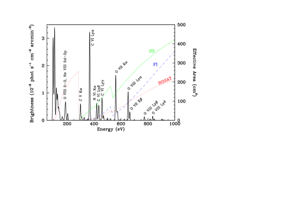
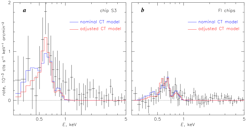
Our resulting model spectrum for geocoronal CT is shown in Fig. 5. That model was then used to simultaneously fit the bright-September S3 and FI data between 250 and 5000 eV using their associated ACIS response functions (see §2.2). Given the limited statistics ($\sim 700$ counts attributable to X-ray emission in the S3 data, and fewer in the FI spectra), we grouped the model emission into four “lines” at 440, 570, 660, and 810 eV; the 440-eV and 810-eV lines are modeled as finite-width Gaussians since they represent several lines spread over a 100-eV and 60-eV range, respectively.

Because of the poor statistics, the only free parameter is the normalization. As can be seen in Fig. 6, overall agreement between the shape of the model spectrum and observation is good, particularly for the O lines which are the most prominent features. The fit shows that carbon emission is overpredicted, however, which may be because of atypical ion abundances, errors in CT cross sections and line yields, or uncertainties in the QE of the ACIS detectors near the extreme limits of their effective energy ranges. Better agreement is obtained when relative ion abundances are adjusted; in the adjusted fit, we reduce the abundances (relative to He-like O VII) of H-like C VI and O VIII by factors of 6 and 2, respectively. When a line is added to fit the putative Mg XI K$\alpha$ feature at 1340 eV, the $F$-test significance is 99.6%.

In fitting the FI and S3 spectra simultaneously, we are implicitly assuming that they recorded the same emission. This is not strictly true because of differing exposures for each chip/ObsID combination, and in fact, if the S3 and FI spectra are fit separately, the S3 brightness comes out somewhat higher than for the FI data. Although within statistical uncertainties, this difference is consistent with the sense of suspected errors in the quantum efficiency of the ACIS chips.

Line brightnesses from the adjusted-abundances fit are listed in Table 7; note that O VII K$\alpha$ and O VIII Ly$\alpha$ are essentially unresolved in the S3 data so their combined brightness is more reliable than the individual values. We also list the corresponding model predictions for an average solar wind (which will be derived in §4.2), which are more than an order of magnitude smaller than observed. As we will discuss in §4.3, based on available solar-wind data, there is good reason to expect a much higher-than-average geocoronal emission level during the September observations, as well as relatively weak C VI emission.

We lastly note that the bright-September S3 spectrum is remarkably similar in shape (and normalization) to the diffuse X-ray background spectra reported by Markevitch et al. (2002) for ObsIDs 3013 and 3419, which observed regions of the sky removed from any bright Galactic structures (see their Fig. 14). Those spectra were fit with a MEKAL thermal model, in both cases yielding a temperature of $T\sim 0.2$ keV. We obtain the same result when fitting that model to our bright-September data.

4.2. Predicted Intensities for Average Solar Wind

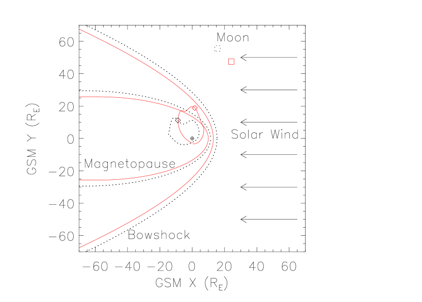
To compare predicted absolute line intensities with observed values, we return to Eq. 1, and write the emissivity as $\epsilon_{il}=v_{c}n_{n}n_{p}f_{O}f_{i}y_{il}\sigma_{i}$, where the ion density, $n_{i}$, is expressed as the solar-wind (proton) density, $n_{p}$, times the relative abundance of oxygen, $f_{O}$, times the ion abundance relative to O, $f_{i}$. As a baseline for comparison with specific Chandra observations, we use average solar-wind parameters in the calculations that follow. As noted before, the average slow-wind velocity $v_{c}$ is 400 km s^-1. Solar wind density is 7 cm^-3 at 1 AU, the fractional O abundance is about 5.6$\times 10^{-4}$ (Schwadron & Cravens, 2000), and relative ion abundances are listed in Table 5. We assume that the ion density inside the magnetosphere is zero, and constant everywhere outside. Using the undisturbed wind density is an approximation, as the wind sweeps around the Earth’s magnetosphere in a wake-shaped structure (see Fig. 7), piling up on the leading edge of the bowshock, with higher-density lower-velocity shocked ions in the magnetosheath, but the resulting errors are comparable to other uncertainties in our model.

The remaining factor in CT emissivity, and the one with the largest uncertainty, is the neutral gas density. We use the analytical approximation of Cravens, Robertson, & Snowden (2001), based on Hodges’ (1994) model of exospheric hydrogen, which is that atomic H density falls off roughly as $(10R_{E}/r)^{3}$, where $R_{E}$ is one Earth radius (6378 km) and $r$ is the geocentric distance. On the leading edge of the magnetosphere, at $r\sim 10R_{E}$, $n_{n}$ is approximately 25 cm^-3. On the flanks, the magnetosphere extends to $r\sim 15R_{E}$.

Figure 7.— Schematic of observation viewing geometry, with dotted curves for the July observations and solid for September. In Geocentric Solar Magnetospheric (GSM) coordinates, Earth is at the origin, $X$ points toward the Sun, and the $XZ$ plane contains the Earth’s magnetic axis. The $Y$ and $Z$ axes thus oscillate with a period of 24-hours, which makes Chandra’s orbit appear non-elliptical. Positions of the magnetosphere and bowshock are approximate and based on the models of (Tsyganenko, 1995, 1989) and (Bennett et al., 1997), respectively. Chandra was barely inside the magnetopause in July, despite its apparent position in this projection.

The brightness of a line $l$ observed by Chandra while looking toward the Moon is given by

$$B_{il}=\frac{1}{4\pi}\int_{0}^{D_{Moon}}\epsilon_{il}(x)dx\;\;\mathrm{phot}\;\mathrm{s}^{-1}\mathrm{cm}^{-2}\mathrm{sr}^{-1}$$ (2)

where $x$ is the distance from Chandra. The neutral gas density, and therefore emissivity, is essentially zero at the distance of the Moon so we can replace $D_{Moon}$ with $\infty$ in the integral. If we also approximate the look direction as being radially outward from Earth, then $dx=dr$ and

$$B_{il} = \frac{1}{4\pi}\int_{r_{min}}^{\infty}n_{n}n_{p}f_{O}f_{i}v_{c}y_{il}\sigma_{i}dr$$ (3)

$$= \frac{v_{c}n_{p}f_{O}f_{i}y_{il}\sigma_{i}n_{n0}}{4\pi}\int_{r_{min}}^{\infty}\left(\frac{10R_{E}}{r}\right)^{3}dr$$ (4)

$$= \frac{v_{c}n_{p}f_{O}f_{i}y_{il}\sigma_{i}n_{n0}}{4\pi}5R_{E}\left(\frac{10R_{E}}{r_{min}}\right)^{2},$$ (5)

where $r_{min}$ is the geocentric distance to the edge of the magnetosphere or the spacecraft’s position, whichever is farther. The brightness of line $l$ for average slow-wind parameters is then

$$B_{il}=9.95\times 10^{14}\left(\frac{10R_{E}}{r_{min}}\right)^{2}y_{il}f_{i}\sigma_{i}\;\;\mathrm{phot}\;\mathrm{s}^{-1}\mathrm{cm}^{-2}\mathrm{sr}^{-1}.$$ (6)

Chandra orbits between about $3R_{E}$ and $20R_{E}$, and the Moon observations were all made near apogee, so $r_{min}=20R_{E}$. (Chandra was in fact very slightly inside the magnetopause in July, but the difference in $r_{min}$ is negligible.) During both July and September, Chandra was looking toward the Moon through the forward flanks pointing slightly toward the leading edge (see Fig. 7), and its orbit was inclined by $\sim 40^{\circ}$. A numerical integration taking into account the non-radial character of Chandra’s viewing angle results in a factor of $\sim 1.5$ increase over the radial approximation. A further slight adjustment for the effects of the shock region (guided by the results of Robertson & Cravens (2003b)) brings the total increase to a factor of two, so that the final prediction for the Chandra observations, assuming a typical slow solar wind, is a line brightness of $B_{il}=5.0\times 10^{14}y_{il}f_{i}\sigma_{i}\;\;\mathrm{phot}\;\mathrm{s}^{-1}\mathrm{cm}^{-2}\mathrm{sr}^{-1}$. The $B_{model}$ values listed in Table 7 are the sums of $B_{il}$ for lines within each line-group.

It is often more convenient to compare predicted and observed counting rates rather than source brightnesses from spectral fits, particularly when energy resolution is limited, as with ROSAT . For an observation subtending a solid angle $\Delta\Omega$, the counting rate is $\Delta\Omega\>\sum_{il}B_{il}A_{il}$, where $A_{il}$ is the instrument effective area at the energy of line $l$ and the sum is over all lines within the chosen energy range. For ACIS, one chip subtends $5.9\times 10^{-6}$ steradian, or 69.8 arcmin², and we find that the predicted ACIS-S3 rate between 511 and 886 eV, encompassing all the He-like and H-like O lines, is $9.0\times 10^{-6}$ cts s^-1 arcmin^-2.

In comparison, the corresponding observed rate from the July S3 data, excluding ObsID 2469, is $34\pm 20\times 10^{-6}$ cts s^-1 arcmin^-2, while the ObsID 2469 rate is $155\pm 49\times 10^{-6}$ cts s^-1 arcmin^-2. The September rate, from the three brightest ObsIDs, is $287\pm 39\times 10^{-6}$ cts s^-1 arcmin^-2, a factor of 32 higher than predicted for an average solar wind, in general agreement, as one would expect, with the results from the spectral fits in §4.1 listed in Table 7.

4.3. Adjustments for Actual Solar Wind

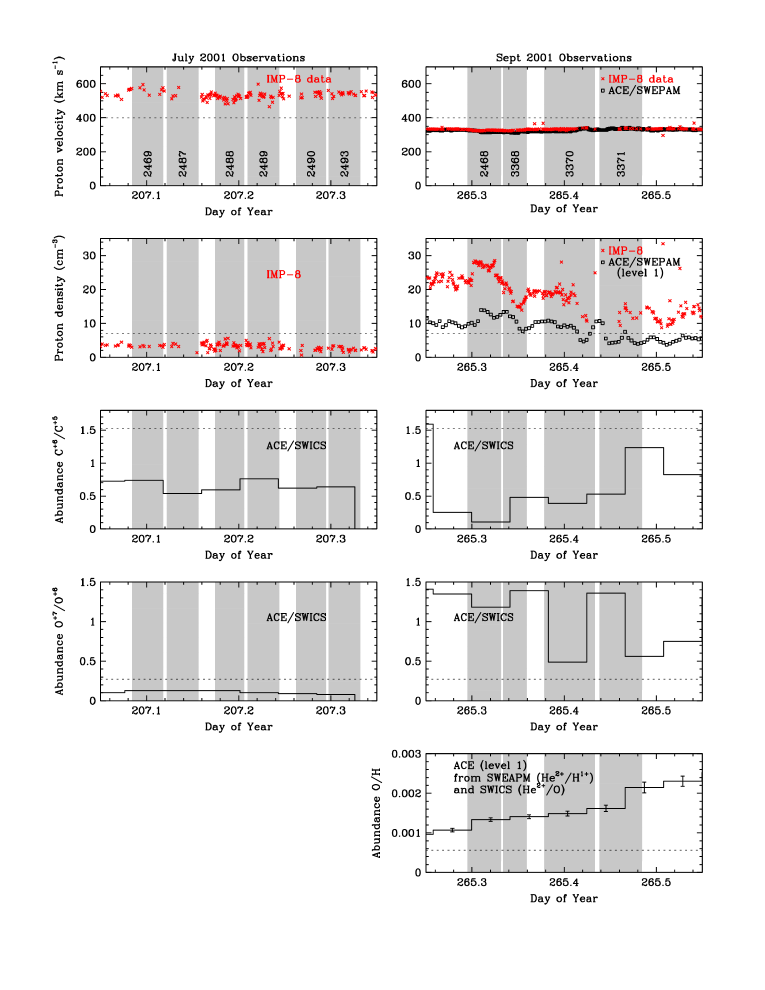
An obvious question raised by the preceding analysis is whether or not the assumptions regarding solar wind parameters are appropriate for the July and September observations. This can be addressed by publically available data from solar monitoring instruments, specifically the Interplanetary Monitoring Platform 8 (IMP-8), and the Solar Wind Electon, Proton, and Alpha Monitor (SWEPAM) and Solar Wind Ion Composition Spectrometer (SWICS) onboard the Advanced Composition Explorer (ACE). Fig. 8 shows the available relevant data, namely the solar wind velocity and density, and various element and ion relative abundances. Horizontal dotted lines denote the average solar-wind parameter values given previously. It is immediately obvious that CT emission rates should be much larger than average in September, and smaller in July.

In July, the wind velocity $v_{c}$ averaged around 530 km s^-1, versus 335 km s^-1 in September. Wind densities, on the other hand, are much higher in September than in July. The proton density measured by IMP-8 in July is $\sim 3.5$ cm^-3, or half the baseline value, while in September the density ranges from $\sim 26$ cm^-3 for the first ObsID (2468) to $\sim 13$ cm^-3 in the last (ObsID 3371). The ACE/SWEPAM densities are about half as large as the densities measured by IMP-8, but are only available in September, and only for level-1 data which are not recommended for scientific analyses. ACE also orbits around the Lagrange L1 point lying 0.01 AU ($\sim 240R_{E}$) toward the Sun, whereas IMP-8 is much closer to the Earth (orbital distance $\sim 35R_{E}$). For all those reasons, we therefore rely on the IMP-8 densities. Note that ACE data plotted in Fig. 8 have been time-shifted to account for wind travel-time to Earth: July data by $1.584\times 10^{6}$ km $/$ 530 km s${}^{-1}=2990$ s, and September data by $1.435\times 10^{6}$ km $/$ 335 km s${}^{-1}=4280$ s. IMP-8 data have at most a few hundred seconds of delay. After these corrections, the time-behavior of the IMP-8 and ACE density data match each other very well.

Oxygen abundance data are not available for July, but the September data show a significant enhancement over average values, by roughly a factor of two during ObsID 2468 and rising to more than a factor of three during ObsID 3371. In July, ACE/SWICS data indicate a relatively lower ionization state than usual for carbon (see Table 5). This is also true of the September data, although the C⁶⁺/C⁵⁺ abundance ratio is more volatile. There is a significant rise in the ratio during ObsID 3371, which might be correlated with the increase in emission above 700 eV associated with especially highly-charged ions during that observation (see Table 3). Overall, the abundance of the C⁶⁺ ions that CT to produce C VI Lyman emission lines is lower than usual, in agreement with the relative weakness of those lines in the September spectra.

ACE/SWICS does not measure the O⁸⁺/O⁷⁺ ratio, but the O⁷⁺/O⁶⁺ ratio, which is usually 20:73 (see Table 5), is less than half that in July and much higher in September. Determining what the absolute ion fractions are can not be done precisely since the wind ions are not really in ionization equilibrium, but based on the tabulations of Mazzotta et al. (1998) we estimate that the O⁶⁺:O⁷⁺:O⁸⁺ relative abundances are roughly 90:10:0 in July and 35:50:15 during most of the September observations, with a drop in ionization level to 60:30:10 during most of ObsID 3370. That drop in the abundance of highly charged oxygen may be largely responsible for the lower X-ray emission observed during ObsID 3370 (see Table 3).

Putting all the above factors together ($v_{c}$, $n_{p}$, $n_{O}/n_{p}$, and $f_{i}$) and assuming that the July oxygen abundance was normal, the CT X-ray intensity between 500 and 900 eV in July should be 0.25 times the baseline intensity, or $2.3\times 10^{-6}$ cts s^-1 arcmin^-2. The predicted bright-September rate is 15 times the baseline rate and 60 times the July rate, or $140\times 10^{-6}$ cts s^-1 arcmin^-2. Considering the model uncertainties, particularly our approximation for the neutral H density distribution, this is very good agreement with the observed quiet-July and bright-September rates of $34\pm 20$ and $287\pm 39\times 10^{-6}$ cts s^-1 arcmin^-2, which are quoted with $1\sigma$ uncertainties.

Figure 8.— Solar wind data for Chandra observations. Gray shading marks the duration of each ObsID. Dotted horizontal lines mark average values for the slow solar wind. Level 1 data from ACE (in September proton density plot) are not considered reliable, but are shown for comparison with IMP-8 data. IMP-8 and ACE proton velocity data in September are essentially coincident. Based on Eq. 1, and the corresponding data plotted here, the September X-ray rates are predicted to be much higher than in July, in agreement with observation.

4.4. Application to ROSAT  Moon Observation

We can also compare predicted and observed rates for the ROSAT  Moon data. Because ROSAT  was in low-Earth orbit, observing perpendicular to the Sun-Earth axis through the flanks of the magnetosphere, $r_{min}=15R_{E}$. (Note that the line brightnesses plotted in Fig. 5 are for this case, with the assumption of average solar wind parameters.) ACE had not yet been launched, but during the time of the observation, 1990 June 29 2:11–2:45 UT, IMP-8 measured $v_{c}=400$ km s^-1 with a slightly elevated proton density of 8.5 cm^-3. $B_{il}$ is then equal to $5.37\times 10^{14}y_{il}f_{i}\sigma_{i}\;\;\mathrm{phot}\;\mathrm{s}^{-1}\mathrm{cm}^{-2}\mathrm{sr}^{-1}$.

Using the ROSAT  PSPC effective area for $A_{il}$, and with $\Delta\Omega=3.0\times 10^{-5}$ steradians for the half-Moon, the observed rate, $\Delta\Omega\>\sum_{il}B_{il}A_{il}$, is then predicted to be 0.0038 cts s^-1, vs the vignetting-corrected dark-side observed value of $\sim 0.20$ cts s^-1 (Schmitt et al., 1991), a difference of roughly a factor of 50. In the units of the ROSAT  All-Sky Survey, the predicted CT rate is $11\times 10^{-6}$ cts s^-1 arcmin^-2, while the observed dark-side rate is nearly $600\times 10^{-6}$ cts s^-1 arcmin^-2.

Given this large discrepancy, we look more closely at the Schmitt et al. (1991) observation. In their Fig. 4 we see that the intensity of full-band SXRB emission surrounding the Moon was $\sim 2000\times 10^{-6}$ cts s^-1 arcmin^-2, which is twice as high as the total rate of $\sim 1000\times 10^{-6}$ cts s^-1 arcmin^-2 listed for the field of view in RASS maps during the observation (RA, Dec $\sim 11^{h}44^{m}30^{s}$, $-03^{\circ}22^{\prime}$). Snowden et al. (1995) also noted this and concluded that “the lunar observation occurred during the time of a strong LTE.” Although IMP-8 data on proton velocity and density do not indicate anything out of the ordinary at that time, we have seen from ACE data during the September 2001 Chandra observations that other wind parameters such as oxygen abundance and ionization level can have a very large effect on net CT emission. We therefore agree that the ROSAT  data indicate an LTE, and deduce that the extra $\sim 1000\times 10^{-6}$ cts s^-1 arcmin^-2 in the measured SXRB rate comprises $\sim 600\times 10^{-6}$ from a large increase in the geocoronal CT rate and $\sim 400\times 10^{-6}$ from the associated transient excess of heliospheric CT emission. The rough equivalence of the geocoronal and heliospheric components of the LTE is consistent with model predictions by Cravens, Robertson, & Snowden (2001).

5. IMPLICATIONS FOR THE SXRB

5.1. Heliospheric Charge Transfer

Although geocoronal CT accounts for much if not most of the X-ray emission during an LTE, and can be of roughly the same intensity as the cosmic X-ray background, its quiescent level is an order of magnitude or more below that of the typical SXRB. Heliospheric CT emission, however, is several times stronger than quiescent geocoronal emission, as was first shown by Cravens (2000), who presented a model for the distribution of neutral H and He within the heliosphere. Neutral gas is depleted near the Sun because of photoionization and charge transfer with H and He in the solar wind, and densities are higher upwind, with respect to the Sun’s relative motion through the Local Interstellar Cloud, than downwind. Densities can be approximated by the relation $n_{n}=n_{n0}e^{-\lambda/r}$, where $n_{n0}$ is the asymptotic neutral density, $r$ is distance from the Sun, and $\lambda$ is the depletion scale.

Outside the heliosphere, in the undisturbed interstellar medium, the neutral H density is 0.20 cm^-3, but behind the shock front the density drops by nearly a factor of two, so that $n_{n0}=0.12$ cm^-3 (Gloeckler et al., 1997). Helium, in contrast, is largely unaffected by the shock, and $n_{n0}=0.015$ cm^-3. Based on the theoretical work of Zank (1999), $\lambda$ for H is approximately 5 AU upwind, 7 AU on the heliosphere flanks, and very roughly 20 AU downwind. He is less depleted near the Sun and has less spatial variation, with $\lambda\sim$ 1 AU. Robertson & Cravens (2003a) have developed a more sophisticated model for the distribution of neutral H and He in all directions, but our predictions of absolute CT emission should not be significantly less accurate; in both cases, the estimated uncertainty is roughly a factor of two or three. Our calculations, however, keep track of each CT emission line and the ROSAT  PSPC effective area for that line energy, which will allow us to draw more specific conclusions regarding the relative strength of emission in various energy bands.

For heliospheric CT emission, Eq. 3 thus becomes

$$B_{il}=\frac{1}{4\pi}n_{p}f_{O}f_{i}v_{c}y_{il}\sigma_{i}n_{n0}\int_{1\>\mathrm{AU}}^{\infty}\left(\frac{1\;\mathrm{AU}}{r}\right)^{2}e^{-\lambda/r}\,dr,$$ (7)

where we again approximate the look direction as radially outward from the Sun. Proton density, $n_{p}$, decreases as the solar wind expands away from the Sun, leading to the $r^{-2}$ factor in the integral. If we isolate the ion-specific terms, $y_{il}f_{i}\sigma_{i}$ (and ignore changes in the abundance of each ion species with distance from the Sun—ions change charge with each CT collision, but the path length for CT is many tens of AU), and evaluate the rest of Eq. 7 using the average solar wind and neutral gas parameters listed previously, we obtain

$$B_{il}=Cy_{il}f_{i}\sigma_{i}\;\;\mathrm{phot}\;\mathrm{s}^{-1}\mathrm{cm}^{-2}\mathrm{sr}^{-1},$$ (8)

where $C$ has units of s^-1 cm^-4 sr^-1 and parametrizes the solar wind density and velocity and the neutral gas distribution along the line of sight. For CT with He, $C=1.76\times 10^{15}$, and for H it equals $4.37\times 10^{15}$, $3.12\times 10^{15}$, and $1.06\times 10^{15}$ when looking upwind, on the flanks, and downwind, respectively. Observations that look through the helium focusing cone downwind of the Sun, where He density is enhanced by roughly a factor of four (Michaels et al., 2002), will see more emission, with $C\sim 10^{16}$. Note, however, that cross sections for He CT with the most important ions are roughly a factor of two smaller than for H CT (see Table 5, which also lists values of $f_{i}$ for the slow wind).

Table 8Model CT Rate Predictions

Neutral	Look	Total ROSAT  Rate
Gas	Direction	($10^{-6}$ cts s-1 arcmin-2)
Helio H	upwind	87
Helio H	flanks	62
Helio H	downwind	21
Helio He	any	16
Helio He	He cone	$\sim 90$
Geo H	upwind	24
Geo H	flanks	11
Geo H	downwind	$\sim 0$

Note. — Results are for look directions within the slow solar wind. ROSAT  always looked through the flanks of the Earth’s magnetosphere; geocoronal rates for upwind and downwind directions are provided for comparison and application to other missions. Heliospheric emission when looking primarily through the fast wind is much lower.

Predicted ROSAT  counting rates from quiescent CT emission are listed in Table 8. The total of geocoronal and heliospheric emission is around $80\times 10^{-6}$ cts s^-1 arcmin^-2, varying by $\pm 30\times 10^{-6}$ cts s^-1 arcmin^-2 depending on look direction through the slow solar wind. The highest rate, roughly $120\times 10^{-6}$ cts s^-1 arcmin^-2, will be observed when looking through the He cone. For observations primarily through the fast wind, the geocoronal component remains the same, while the He and especially H heliospheric components will be significantly reduced, yielding a total of $\sim 25\times 10^{-6}$ cts s^-1 arcmin^-2. For comparison, typical RASS rates away from bright Galactic structures are 600, 400, and 100 $\times 10^{-6}$ cts s^-1 arcmin^-2 for the full, R12, and R45 energy bands, respectively. For lines of sight mostly through the slow wind (which is most of the sky during solar maximum, when the ROSAT  background maps were conducted), our model therefore predicts that combined quiescent geocoronal and heliospheric CX emission accounts for roughly 13% of the total SXRB measured by ROSAT , 11% of the R12-band emission, and one-third of the R45-band emission. Overall uncertainty in our predictions is roughly a factor of two.

Slightly more than half of the total CT emission ($\sim 55$%) is predicted to be in the R12 band, which is consistent with the observation that the ROSAT  LTEs appear most strongly in the R12 band (Snowden et al., 1995). The true R12-band emission is almost certainly even higher, however, because of the known incompleteness of our CT spectral model. Although we model Li-like O VI and Ne VIII emission, there is additional $L$-shell ($n\rightarrow 2$) CT emission, mostly in the R12 band, resulting from Li-like and lower charge states of Mg, Si, S, Ar, and Fe. Although more difficult to model, these heavier elements have significant abundance (in sum, approximately the same as for bare and H-like C (Schwadron & Cravens, 2000)), and they have been invoked to explain much of the low-energy emission seen in comets (Krasnopolsky, 2004).

Also note that some of the SXRB recorded in the RASS comes from point sources which could not be resolved by ROSAT –Markevitch et al. (2002) estimate 20%—so the fraction of the “true”, i.e., diffuse, SXRB arising from CT is correspondingly higher. Whatever the average level of CT emission is, we expect that it may well be the dominant contributor to the SXRB in some low-intensity fields, particularly in the R45 (3/4-keV) band. If so, CT emission will have a significant impact on our understanding of the SXRB and models of the local interstellar medium, particularly the Local Bubble.

5.2. Once and Future Data

ROSAT , of course, is not the only X-ray satellite affected by CT emission; any X-ray observation made from within the solar system will be impacted. Variations in the strength of background O emission have been noted (tentatively) in repeated Chandra observations of MBM 12, a nearby dark molecular cloud that shadows much of the SXRB (R. J. Edgar et al., in preparation), and in XMM-Newton observations of the Hubble Deep Field North, which also showed variable Ne and Mg emission (S. L. Snowden, 2004, private communication). Such variations may be important when observing weak extended sources such as clusters where background determinations are critical.

With future missions having much better energy resolution, such as ASTRO-E2 with its 6-eV-FWHM-resolution microcalorimeter array (Stahle et al., 2003), one should be able to see differences in background spectra between areas of the sky corresponding to low and high solar latitudes (around solar minimum) because of the difference in ionization levels between the slow and fast solar winds. It should also be easy to identify spectral features indicative of CT, such as an anomalously strong O VII K$\alpha$ forbidden line ($1s2s$ ${}^{3}S_{1}\rightarrow 1s^{2}$ ${}^{1}S_{0}$). When excited by CT, that line is several times stronger than the resonance line ($1s2p$ ${}^{1}P_{1}\rightarrow 1s^{2}$ ${}^{1}S_{0}$), completely unlike their ratio in thermal plasmas (Kharchenko et al., 2003). Other signatures of CT are the high-$n$ Lyman transitions of O and C, which are strongly enhanced relative to Ly$\alpha$. Indeed, there are hints of high-$n$ O Lyman lines in a short (100 sec) microcalorimeter observation (McCammon et al., 2002). There is also a strong feature at $\sim 67.4$ Å (184 eV) in the Diffuse X-Ray Spectrometer (DXS) spectrum of the SXRB (Sanders et al., 2001) which cannot be reproduced by thermal plasma models. A promising explanation is CT emission at 65.89 and 67.79 Å (188.16 and 182.89 eV) from Li-like Ne VIII $1s^{2}5d\rightarrow 1s^{2}2p$ and H-like O VIII $5d,5s\rightarrow 2p$ transitions, which are the strongest CT features within the 148-284-eV DXS energy range (see Fig. 5, and note that the plotted resolution is very similar to that for ASTRO-E2 and DXS).

Although variability in foreground emission, whether from changes in the solar wind or in the position of the observing spacecraft with respect to the magnetosphere and heliosphere, can be an annoying complication when analyzing extended sources, variations of CT emission in time and space also provide opportunities to learn more about the solar wind, geocorona, and heliosphere. Data from Chandra and XMM-Newton will provide important constraints on our models of CT emission, and future missions such as ASTRO-E2 should permit definitive tests. Given the unavoidable and rather large uncertainties in current theoretical models, observational data will be critical in this endeavor.

6. CONCLUSIONS

As described in this paper, we have detected significant time-variable soft X-ray emission in Chandra observations of the dark side of the Moon which is well explained by our model of geocoronal charge transfer. The observed brightness ranged from a maximum of $\sim 2\times 10^{-6}$ phot s^-1 arcmin^-2 cm^-2, with most of the emission between 500 and 900 eV, to a minimum at least an order of magnitude lower. Predicted intensities, which are based in part on detailed solar wind data, match observation to within a factor of two, which is within the model uncertainty. Emission from O VII K$\alpha$, O VIII Ly$\alpha$, and a blend of high-$n$ O VIII Lyman lines is detected with high confidence, as well as probably Mg XI K$\alpha$ and perhaps high-$n$ emission from C VI. We also include estimates of heliospheric emission and find that the total charge transfer emission amounts to a substantial fraction of the soft X-ray background, roughly one-third of the rate measured in the ROSAT  R45 band. Future observations with microcalorimeter detectors should allow much more accurate assessments of the contribution of charge transfer emission to the SXRB because of its unique spectral signatures.

References

- Bennett et al. (1997) Bennett, L., Kivelson, M. G., Khurana, K. K., Frank, L. A., & Paterson, W. R. 1997, J. Geophys. Res., 102, 26927
- Biller, Plucinsky, & Edgar (2002) Biller, B., Plucinsky, P., & Edgar, R. 2002, (http://asc.harvard.edu/cal/, ”ACIS”, ”Background”, ”Event Histogram Files”)
- Cox (1998) Cox, D. P. 1998, in The Local Bubble and Beyond, ed. D. Breitschwerdt, M. J. Freyberg, and J. Trümper (Berlin:Springer), 121
- Cravens (2002) Cravens, T. E. 2002, Science, 296, 1042
- Cravens (2000) Cravens, T. E. 2000, ApJ, 532, L153
- Cravens (1997) Cravens, T. E. 1997, Geophys. Res. Lett., 24, 105
- Cravens, Robertson, & Snowden (2001) Cravens, T. E., Robertson, I. P., & Snowden, S. L. 2001, J. Geophys. Res., 106, 24883
- Freyberg (1998) Freyberg, M. J. 1998, in The Local Bubble and Beyond, ed. D. Breitschwerdt, M. J. Freyberg, and J. Trümper (Berlin:Springer), 113
- Freyberg (1994) Freyberg, M. J. 1994, PhD thesis, LMU München
- Gloeckler et al. (1997) Gloeckler, G. J., Fisk, L. A., & Giess, J. 1997, Nature, 386, 374
- Greenwood et al. (2001) Greenwood, J. B., et al. 2001, Phys. Rev. A, 63, 62707
- Harel, Jouin, & Pons (1998) Harel, C., Jouin, H., & Pons B. 1998, At. Data and Nucl. Data Tables, 68, 279
- Hodges (1994) Hodges, R. R., Jr. 1994, J. Geophys. Res., 99, 23229
- Johnson et al. (2000) Johnson, W. R., Savukov, I. M., Safronova, U. I., & Dalgarno, A. 2000, ApJS, 141, 543
- Kharchenko & Dalgarno (2001) Kharchenko, V., & Dalgarno, A. 2001, ApJ, 554, L99
- Kharchenko & Dalgarno (2000) Kharchenko, V., & Dalgarno, A. 2000, J. Geophys. Res., 105, 18351
- Kharchenko et al. (2003) Kharchenko, V., Rigazio, M., Dalgarno, A., & Krasnopolsky, V. A. 2003, ApJ, 585, L73
- Krasnopolsky (2004) Krasnopolsky, V. A. 2004, Icarus, 167, 417
- Krasnopolsky & Mumma (2001) Krasnopolsky, V. A., & Mumma, M. J. 2001, ApJ, 549, 629
- Lisse et al. (2001) Lisse, C. M., Christian, D. J., Dennerl, K., Meech, K. J., Petre, R., Weaver, H. A., & Wolk, S. J. 2001, Science, 292, 1343
- Lisse et al. (1996) Lisse, C. M., et al. 1996, Science, 274, 205
- Markevitch (2002) Markevitch, M. 2002, (http://asc.harvard.edu/cal/, ”ACIS”, ”Background”, ”Particle Background Observations”)
- Markevitch et al. (2002) Markevitch, M., et al. 2002, ApJ, 583, 70
- Mazzotta et al. (1998) Mazzotta, P., Mazzitelli, G., Colafrancesco, S., & Vittorio, N. 1998, A&AS, 133, 403
- McCammon et al. (2002) McCammon, D., et al. 2002, ApJ, 576, 188
- McCammon & Sanders (1990) McCammon, D., & Sanders, W. T. 1990, ARA&A, 28, 657
- Michaels et al. (2002) Michaels, J. G., et al. 2002, ApJ, 568, 385
- Rigazio, Kharchenko, & Dalgarno (2002) Rigazio, M., Kharchenko, V., & Dalgarno, A. 2002, Phys. Rev. A, 66, 64701
- Robertson & Cravens (2003a) Robertson, I. P., & Cravens, T. E. 2003a, J. Geophys. Res., 108, 8031
- Robertson & Cravens (2003b) Robertson, I. P., & Cravens, T. E. 2003b, Geophys. Res. Letters, 30, 1439
- Sanders et al. (2001) Sanders, W. T., Edgar, R. J., Kraushaar, W. L., McCammon, D., & Morgenthaler, J. P. 2001, ApJ, 554, 694
- Schmitt et al. (1991) Schmitt, J. H. M. M., Snowden, S. L., Aschenbach, B., Hasinger, G., Pfeffermann, E., Predehl, P., & Trümper, J. 1991, Nature, 349, 583
- Schwadron & Cravens (2000) Schwadron, N. A., & Cravens, T. E. 2000, ApJ, 544, 558
- Smith et al. (2003) Smith, E. J., et al. 2003, Science, 302, 1165
- Snowden et al. (1995) Snowden, S. L., et al. 1995, ApJ, 454, 643
- Snowden et al. (1997) Snowden, S. L., et al. 1997, ApJ, 485, 125
- Stahle et al. (2003) Stahle, C. K., et al. 2003, Proc. SPIE, Vol. 4851, 1394
- Tsyganenko (1995) Tsyganenko, N. A. 1995, J. Geophys. Res., 100, 5599
- Tsyganenko (1989) Tsyganenko, N. A. 1989, Planet. Space Sci., 37, 5
- Vikhlinin (2001) Vikhlinin, A. 2001, (http://asc.harvard.edu/cal/, ”ACIS”, ”Background”, ”Reducing ACIS Quiescent Background”)
- Zank (1999) Zank, G. P. 1999, Space Sci. Rev., 89, 413