The Far-Ultraviolet Spectra of TW Hya. II. Models of H₂ Fluorescence in a Disk¹

Abstract

We measure the temperature of warm gas at planet-forming radii in the disk around the classical T Tauri star (CTTS) TW Hya by modelling the H₂ fluorescence observed in HST/STIS and FUSE spectra. Strong Ly$\alpha$ emission irradiates a warm disk surface within 2 AU of the central star and pumps certain excited levels of H₂. We simulate a 1D plane-parallel atmosphere to estimate fluxes for the 140 observed H₂ emission lines and to reconstruct the Ly$\alpha$ emission profile incident upon the warm H₂. The excitation of H₂ can be determined from relative line strengths by measuring self-absorption in lines with low-energy lower levels, or by reconstructing the Ly$\alpha$ profile incident upon the warm H₂ using the total flux from a single upper level and the opacity in the pumping transition. Based on those diagnostics, we estimate that the warm disk surface has a column density of $\log N($H${}_{2})=18.5^{+1.2}_{-0.8}$, a temperature $T=2500^{+700}_{-500}$ K, and a filling factor of H₂, as seen by the source of Ly$\alpha$ emission, of $0.25\pm 0.08$ (all 2$\sigma$ error bars). TW Hya produces approximately $10^{-3}$ $L_{\odot}$ in the FUV, about 85% of which is in the Ly$\alpha$ emission line. From the H I absorption observed in the Ly$\alpha$ emission, we infer that dust extinction in our line of sight to TW Hya is negligible.

1 INTRODUCTION

Classical T Tauri Stars (CTTSs) are roughly solar-mass pre-main sequence (PMS) stars that are accreting gas from their circumstellar disks. The extent and mass of dust in disks have been determined from IR spectral energy distributions (SEDs) and imaging (see review by Zuckerman, 2001). Cold gas at large radii is traced by observations of molecules such as CO and HCN (e.g., Aikawa et al., 2002). Warmer neutral and ionized gases are used as diagnostics of accretion (e.g., Gomez de Castro & Lamzin, 1999; Johns-Krull & Gafford, 2002). However, observing the gas in the disk close to the star, which is important for the formation and evolution of planets, has been difficult. Gas at these radii can induce planet migration (Goldreich & Tremaine, 1979), dampen the eccentricity of terrestrial planets (Agnor & Ward, 2002), and is neccessary for accretion onto giant planets (Lissauer, 1993).

In search of gas at planet-forming radii, Calvet et al. (1991) investigated the formation of CO overtone lines at 2.3 $\mu$m in disks around CTTSs. These models predict that CTTSs as a group should show both CO emission and absorption, while Herbig Ae/Be stars should show CO in emission. Using high spectral resolution observations, Carr et al. (1993) showed that the CO overtone emission from the probable Herbig Ae/Be star WL 16 arises in the inner disk, confirming the prediction of Calvet et al. (1991). Najita et al. (1996) find the same result for the Herbig Ae/Be star 1548C27. However, broader searches at high spectral resolution for CO overtone emission or absorption from CTTSs generally find no evidence for contributions to these lines from the disks around these stars (Casali & Eiroa, 1996; Johns-Krull & Valenti, 2001a). On the other hand, Najita, Carr, & Mathieu (2003) find that CO fundamental emission near 4.6 - 4.9 $\mu$m is common among CTTSs. They suggest that overtone emission has not been detected at the observed CO temperatures (1100 – 1300 K), mainly because the overtone bands have much lower transition rates. However, CO is not expected to be the dominant gas constituent in the disks around CTTSs, and it is the major component of the gas, H₂, that we seek to probe here.

Previous observations of H₂ have not provided a clear picture of the gas in the disk. Thi et al. (2001) detected cold H₂ emission in the pure rotational S(0) and S(1) lines from ISO observations of a large sample of CTTSs, Herbig Ae/Be stars, and debris-disk stars. However, in ground-based observations of the S(1) and S(2) lines, using much smaller apertures than ISO, Richter et al. (2001) and Sheret et al. (2003) did not detect any H₂ emission from some of the same sources, indicating that the emission is probably extended. On the other hand, the emission in the H₂ 1-0 S(1) transition detected by Bary, Weintraub, & Kastner (2003) in Phoenix spectra of 4 T Tauri stars is narrow and centered at the radial velocity of the stars, presumably formed in low-velocity circumstellar gas.

While H₂ lines in the IR are typically weak and are observed against a strong dust continuum, fluorescent H₂ lines dominate the far-ultraviolet (FUV) spectrum of CTTSs at wavelengths longward of Ly$\alpha$. Ardila et al. (2002a) found that narrow H₂ lines can be blueshifted by up to 20 km s^-1 in HST/GHRS spectra of CTTSs, observed with a $2\arcsec\times 2\arcsec$ aperture. High-resolution echelle and long-slit spectroscopy with HST/STIS is providing the critical data needed to identify the source of the H₂ emission. Observations of T Tau reveal two components of H₂ emission. Saucedo et al. (2003) and Walter et al. (2003) detect off-source UV H₂ emission, that is pumped near line-center of Ly$\alpha$, and most likely produced where stellar outflows shock the surrounding ambient molecular material. The same set of fluorescent H₂ lines are detected in low-excitation HH objects such as HH43 and HH47 (Schwartz, 1983; Curiel et al., 1995), suggestive of a similar excitation mechanism. Walter et al. (2003) find that the on-source H₂ emission is photoexcited by a much broader Ly$\alpha$ emission line, likely produced by the accretion shock at the surface of T Tau.

In Herczeg et al. (2002, hereafter Paper I), we presented observations of H₂ fluorescence in the UV spectrum of TW Hya obtained with HST/STIS and FUSE. Several lines of evidence suggested a disk origin for the H₂ emission: (i) the H₂ emission is not spatially extended beyond a point source in the cross-dispersion direction, (ii) the H₂ lines are emitted interior to TW Hya’s wind because emission in one H₂ line is supressed by C II wind absorption, (iii) the H₂ line centroids have the same radial velocity as the photospheric lines of TW Hya, (iv) no H₂ absorption is detected against the Ly$\alpha$ emission, and (v) the TW Hya Association is isolated from large reservoirs of interstellar molecular material, making a circumstellar origin for the H₂ emission unlikely. Because the H₂ emission is not extended beyond a point source, the spatial resolution of HST/STIS restricts the emitting region to be within 2 AU of the star.

Analysis of on-source IR H₂ emission lines to date has been limited because typically only one or two lines are observed. The IR lines could be excited by shocks, UV fluorescence, X-rays, or thermal heating. In contrast, over 140 H₂ lines from 19 different upper levels are detected in the FUV spectrum of TW Hya. The excitation of H₂ can be determined from relative line strengths in this rich spectrum either by measuring self-absorption in low excitation members of individual fluorescent progressions or by using an assumed Ly$\alpha$ profile to reconstruct initial level populations in various pumping transitions.

In this paper, we calculate the temperature of warm gas at planet-forming distances by modelling warm H₂ in a disk around TW Hya. We use the H₂ emission to reconstruct the Ly$\alpha$ profile incident on the fluoresced H₂. The observed Ly$\alpha$ profile differs from the incident profile because of interstellar absorption along our line of sight to TW Hya. We discuss the strength of Ly$\alpha$ emission and its affect on the circumstellar disk.

2 PROPERTIES OF TW HYA

TW Hya is the namesake of the 10 Myr old TW Hya Association (TWA), which most likely originated in the Sco-Cen OB association (Mamajek, Lawson, & Feigelson, 2000). TW Hya is one of the oldest known stars still in the CTTS phase, and its mass accretion rate of about $2-3\times 10^{-9}M_{\odot}$ yr^-1 is lower than the mass accretion rate of most of the 1–2 Myr old CTTSs that are found in Taurus (Kenyon & Hartmann, 1995). From PMS evolutionary tracks, Webb et al. (1999) estimate that TW Hya has a mass of $0.7$ $M_{\odot}$ and a radius of $1.0$ $R_{\odot}$. Gaseous material is often associated with young stars, but is not found in the nearby TWA, so the extinction is low. The TWA is located at a distance of approximately 56 pc (Webb et al., 1999), compared with 140 pc for Taurus. Consequently, TW Hya is by far the brightest known CTTS in the UV and in X-rays. Most of the UV radiation from TW Hya is presumably produced at the accretion shock. The disk is viewed face-on (e.g., Zuckerman et al., 1995; Alencar & Batalha, 2002), which prevents signficant Keplerian broadening in the H₂ line profiles. The disk mass is roughly $(1.5-3)\times 10^{-2}$ $M_{\odot}$ (Wilner et al., 2000; Trilling et al., 2001) and extends more than 225 AU from the star (e.g. Krist et al., 2000). Based on estimates of the stellar mass, radius, and rotation period of TW Hya, Johns-Krull & Valenti (2001b) calculate that the disk at 6 $R_{*}$ corotates with the stellar surface. In the Shu et al. (1994) model, the disk is truncated at corotation. Weinberger et al. (2002) estimate from modelling the IR SED of TW Hya that the dust in the disk is truncated at about 11 $R_{*}$. In their models of the IR SED, Calvet et al. (2002) found an underabundance micron-sized dust grains within 4 AU of TW Hya. Figure 1 shows a schematic model of TW Hya and its disk.

Since the mass accretion rate of CTTSs can vary, we calculate the mass accretion rate at the epoch when we observed TW Hya. We then proceed to estimate the extinction using H I absorption against Ly$\alpha$ emission and the SED of the NUV continuum that is produced in an accretion shock. The observations discussed in this paper were described in Paper I and are listed in Table 1.

2.1 Mass Accretion Rate

The strong excess blue and UV emission from CTTSs can be modelled as emission from shocks at accretion footpoints on the star, which leads to estimates of the mass accretion rate. We estimate the accretion rate of TW Hya by following the method of Valenti, Basri, & Johns (1993), who modelled observed blue spectra with the sum of a photospheric template and emission from a slab of hot isothermal hydrogen to crudely simulate emission from the accretion shock.

We use the HST/STIS spectrum of the K7 weak-lined TTS V819 Tau (see Table 1), spanning 1100–6000 Å, as a non-accreting template for the photospheric emission from TW Hya. For V819 Tau we adopt a visual extinction of $A_{V}=1.52$, which is the average of values determined by Kenyon & Hartmann (1995) and White & Ghez (2001). We then use the interstellar extinction law of Cardelli et al. (1989) to remove the effects of extinction from the observed spectrum of V819 Tau. The NUV and FUV emission from V819 Tau is much fainter than that of TW Hya, and is not significant in this analysis.

The spectrum of the model slab is determined by the slab temperature $T$, density $n$, thickness $l$, extinction $A_{V}$ towards the slab, and a slab surface area parameter $\delta$, as described in Valenti et al. (1993). The slab surface area parameter $\delta$ corresponds to the fraction of the stellar surface area covered by accretion-related emission, and is calculated from the scale factor applied to the slab spectrum. The scaling factor between the non-accreting template star and TW Hya is another free parameter. We find the best-fit model parameters by fitting the synthetic slab spectrum plus the scaled template spectrum to the NUV and optical spectrum of TW Hya, minimizing $\chi^{2}$ using the amoeba function in IDL, which is based on the downhill simplex minimization method. The best-fit parameters for the slab are $A_{V}=0.0$, $T=9900$ K, $n=1.7\times 10^{14}$ cm^-3, $l=125$ km, $\delta=0.008$, and a template scaling factor of 1.18.

Figure 2 shows our fit to the optical spectrum of TW Hya, after subtracting the scaled template spectrum of V819 Tau. The accretion continuum calculated in this model is consistent with the observed NUV continuum. However, the observed continuum flux rises shortward of 1700 Å, which could result from (i) an H₂ dissociation continuum produced by electron collisions (Liu & Dalgarno, 1996), (ii) H₂ fluorescence pumped by the FUV continuum, or (iii) by a hot accretion or activity component. The SED of the FUV continuum is similar to the continuum observed in HH2, which is probably produced by H₂ dissociation (Raymond et al., 1997). However, the FUV continuum of TW Hya appears smooth and does not show strong H₂ emission lines at 1054 Å and 1101 Å, which are detected towards HH2.

Assuming that half of the potential energy of the accreting gas is converted into hydrogen continuum emission², then the mass accretion rate of TW Hya can be estimated by

$$\dot{M}_{*}=\frac{1.25R_{*}L_{\rm slab}}{GM_{*}},$$ (1)

where $L_{\rm slab}=3.5\times 10^{-10}$ erg cm^-2 s^-1 is the slab flux integrated over all wavelengths. The leading factor of 1.25, derived by Gullbring et al. (1998) for a magnetospheric accretion geometry, replaces the factor of 2 from a spherical accretion geometry. We adopt $0.7~{}M_{\odot}$ and $1.0~{}R_{\odot}$ for the mass and radius of TW Hya (Webb et al., 1999). Uncertainties in the stellar mass, radius, and distance are all of order 20%. We calculate an accretion rate onto the star of $\dot{M}\approx 2\times 10^{-9}$ $M_{\odot}$ yr^-1, which is consistent with the accretion rate of $2\times 10^{-9}$ $M_{\odot}$ yr^-1 estimated by Alencar & Batalha (2002) using a similar method, and is larger than the accretion rate of $5\times 10^{-10}$ $M_{\odot}$ yr^-1 estimated by Muzerolle et al. (2000) using an analysis of the H$\alpha$ line.

2.2 Extinction to TW Hya

In this section, we argue that the extinction to TW Hya is negligible by measuring the hydrogen column density directly from the shape of the observed Ly$\alpha$ line, and then using an ISM extinction law to infer the dust extinction. This argument does not necessarily imply that the extinction towards the warm H₂ is negligible, because some dust could be mixed with the warm H₂, leading to extinction of H₂ fluxes without any extinction of the stellar or accretion emission. We will discuss this possibility in §5.

Figure 3 shows the observed Ly$\alpha$ profile, which is likely produced in an accretion column, contains a dark, broad absorption feature that extends from +200 km s^-1 to -500 km s^-1. The absorption is produced by H I in the wind and in interstellar and circumstellar material. Because circumstellar and interstellar absorption are indistinguishable in our data, we model these two features with a single absorption feature. All UV spectra of CTTSs show similar wind absorption in Mg II (Ardila et al., 2002b), so the star must be occulted by the outflow, regardless of inclination angle.

In the following analysis, we fit two Gaussian emission profiles and either one or two Voigt absorption profiles to the observed Ly$\alpha$ profile. The intrinsic emission profile is assumed to be a double-Gaussian profile, and the parameters of the Gaussians are allowed to vary to best fit the observed profile when combined with the absorption. Based on the widely separated wind and interstellar absorption features observed in the O I 1302 Å, C II 1334 Å, and Mg II 2795 Å lines, the interstellar and wind absorption components towards TW Hya must be centered at $v=0$ and $-130$ km s^-1, respectively. For the interstellar component we assume a Doppler parameter of $b=11$ km s^-1, which corresponds to a temperature of 7000 K that is typical of the local (warm) ISM (Redfield & Linsky, 2000). An interstellar column density is then determined by fitting the absorption longward of line center, where any wind absorption should be negligible. The wind absorption extends to a velocity of at least -500 km s^-1, and likely has a large Doppler parameter due to velocity gradients along our line of sight. Given these assumptions, the interstellar neutral hydrogen column density in our line of sight is $\log N($H I$)=19.05\pm 0.15$ (Fig. 3). The upper limit of the column density in the wind is $N($H I$)<19.4$ for Doppler parameters $b>25$ km s^-1

In a more conservative test to find the upper limit to the hydrogen column density, we fit the Ly$\alpha$ absorption with a single component, effectively combining any interstellar and wind absorption. We vary the central wavelength of the absorption and set a low Doppler parameter parameter, so that the damping wings generate the width of the absorption profile. Figure 4 shows that the maximum possible column density consistent with the data is $\log N($H I$)=19.75$.

The conservative upper limit of the hydrogen column density towards TW Hya is therefore $\log N($H$)<19.75$. In the only previous measurement of $N$(H I) to TW Hya, Kastner et al. (1999) used X-ray spectral energy distributions from ROSAT and ASCA to estimate higher column densities of $\log N($H I$)=20.5\pm 0.4$ and $21.4\pm 0.1$, respectively. However, the X-ray analyses are highly reliant on the accuracy of plasma codes. Kastner et al. (1999) estimate the hydrogen column density by assuming solar abundances and using a two-temperature emission measure rather than a differential emission measure distribution. However, in their analysis of the Chandra X-ray spectrum of TW Hya, Kastner et al. (2002) found that the abundances show an inverse-FIP effect. We further note that the sensitivity and flux calibration of ROSAT and ASCA are relatively poor at soft energies, where absorption from H I ionization is measured. Figure 4 shows that the absorption calculated for the Ly$\alpha$ line for $\log N($H I$)=20.5$ is signficantly broader than the observed absorption profile. Our comparison of the calculated transmission function with the observed Ly$\alpha$ profile provides a much simpler and more direct test of hydrogen column density than the X-ray analyses. The discrepancy between the UV and X-ray measurements of N(H) could in principle be due to a variable circumstellar absorber, which Kastner et al. (1999) invoked to explain the order of magnitude discrepancy in calculations of N(H) from ASCA and ROSAT. However, the many ultraviolet observations of TW Hya by IUE, HST/STIS, and FUSE, which are widely spaced in time, show no evidence for large fluctuations in extinction.

We estimate an H₂ column density in our line of sight to TW Hya with FUSE, as the bandpass contains many H₂ transitions from low rotational levels of the ground electronic state, which are often seen in absorption due to the ISM at temperatures typically $\sim 100$ K (Rachford et al., 2002). H₂ absorption lines from $\hbox{$v^{\prime\prime}$}=0,\hbox{$J^{\prime\prime}$}=0,1,2,3,5$ can in principle be observed against O VI emission (e.g. Roberge et al., 2001). The O VI profiles are noisy (see Fig. 5), but we estimate an upper limit of $\log N($H${}_{2})<18$ by calculating the transmission percentage for a range of temperatures and column densities, meaning the molecular fraction of H towards TW Hya is very low.

When we convert total hydrogen column density, $N$(H I)+$2N($H${}_{2})=N($H), to a reddening using the interstellar relationship of Bohlin, Savage, & Drake (1978),

$$\frac{N({\rm HI}+{\rm H}_{2})}{E(B-V)}=5.8\times 10^{21}{\rm cm}^{-2},$$ (2)

we find that the reddening toward TW Hya is $E(B-V)=A_{V}/R_{V}<0.01$, where $R_{V}$ is a dimensionless parameter that ranges between 2.5–6, depending on the size distribution of dust grains. Significant deviations from the assumed dust-to-gas ratio can occur in star-forming regions such as $\rho$ Oph, in which the dust grains are likely larger than they are in the ISM. However, the low molecular fraction towards TW Hya is consistent with a low extinction (Savage et al., 1977; Rachford et al., 2002), and is not consistent with material found towards star-forming regions. We conclude that this relationship provides a reasonable estimate of the extinction along our sightline to TW Hya. Even if the dust-to-gas ratio along the line of sight to TW Hya were for some reason enhanced by an order of magnitude, then dust extinction would reduce the brightness of TW Hya by a factor of 2 and have only a 20% effect on the relative fluxes between 1200 Å and 1650 Å.

Inspection of the NUV continuum (Fig. 6) confirms the small extinction to TW Hya. If we assume that the NUV continuum is produced in an isothermal slab, as modelled in §2.1, then it can be well fitted with a hydrogen continuum only for extinctions $A_{V}<0.2$. As noted in §2.1, an accretion continuum best fits the NUV continuum for $A_{V}=0.0$.

3 MODELLING H₂ LINE FLUXES

In Paper I, we measured a total line emission flux of $1.94\times 10^{-12}$ erg s^-1 cm^-2 by summing 146 H₂ emission lines in the 19 progressions (the set of R and P transitions from a common upper level) listed in Table 2. Most of these lines are Lyman-band transitions fluoresced by the strong, broad Ly$\alpha$ emission line.

Wood, Karovska, & Raymond (2002) discovered in their analysis of HST/STIS observations of Mira B that H₂ fluxes weaken towards short wavelengths because of increasing H₂ line opacities. This occurs because shorter wavelength lines are transitions to low energy levels, which are more populated than higher levels. Figure 7 demonstrates that the same effect occurs in the H₂ fluorescence sequences detected towards TW Hya. In most sequences, fluxes in many H₂ emission lines at short wavelengths are weaker than predicted from theoretical branching ratios because of significant absorption in the same transitions. Transitions from levels with low excitation energies, such as $v^{\prime}$=0, $J^{\prime}$=1, have significant optical depth below 1300 Å, but this does not happen for transitions from levels with large excitation energies such as $v^{\prime}$=4, $J^{\prime}$=18 (see Fig. 7). The $v^{\prime}$=4, $J^{\prime}$=18 level does not have any downward transitions with significant opacity in the STIS bandpass.

Following the Monte Carlo method of Wood et al. (2002), we compute H₂ opacities by modelling H₂ fluorescence in a 1D isothermal plane-parallel atmosphere of H₂ irradiated by Ly$\alpha$ photons. We assume complete frequency and angular redistribution when photons scatter in the slab. Forty-one wavelength grid points across each H₂ line profile track differences in escape probability across the line profile because because a photon that scatters into the wings of a line escapes from a slab more easily than a photon at line center. A Ly$\alpha$ photon enters the slab at an angle $\theta$ with respect to the slab surface normal and photoexcites an H₂ molecule. The H₂ molecule quickly de-excites to the ground electronic state through one of the many available routes, or dissociates with a probability $P_{Dis}$ [listed in Table 2, calculated by Abgrall, Roueff, & Drira (2000)]. Depending on the optical depth of H₂ in the lower level of the downward transition, the resulting photon may be temporarily absorbed by another H₂ molecule or may emerge from either side of the slab at an angle $\phi$ with respect to the normal. In our simple model, H₂ line photons created fluorescently in the slab either escape, are converted to another H₂ line in the same progression, or dissociate an H₂ molecule. No other photon processes are considered. We tabulate photons that exit the slab on the Ly$\alpha$ entry side (reflected photons) and opposite side (transmitted photons) using 40 bins of equal solid angle on each side of the slab. We refer the reader to Wood et al. (2002) for further details of this Monte Carlo code.

We use the term “model” to refer to the simulated plane-parallel atmosphere described in the preceding paragraph, and the term “geometry” to refer to the morphology of the H₂ around the Ly$\alpha$ emission source. In the context of the model, the H₂ line fluxes depend on the temperature and column density of the slab, the angle of incidence $\theta$ of the Ly$\alpha$ photon into the disk, the outward angle $\phi$ of the emerging photon, the side of the slab from which the photon escapes, and the optical depth of the transition. We assume that extinction is negligible in the slab and in any interstellar material. Figure 8 shows two possible geometries that we use to approximate a thick disk and a thin disk. The term “thick disk” applies to a star-disk geometry in which most of the H₂ illuminated by Ly$\alpha$ is at the inner edge of the disk. The term “thin disk” applies to a geometry in which most of the H₂ illuminated by Ly$\alpha$ is at the disk surface. In this section and §4, we present detailed results for the thick disk geometry that reproduces the data well. In this adopted geometry, Ly$\alpha$ photons enter the slab normally ($\theta=0^{\circ}$), and the H₂ photons that we observe emerge at an angle $\phi=76^{\circ}-79^{\circ}$ to the normal. This choice is intended to present one approximation of a plausible disk geometry for which we can present detailed results, and is not meant to exclude other geometries. In §5, we present general results for many geometries to demonstrate that our primary result, the temperature of the H₂ gas, is relatively insensitive to geometries, including those that are significantly different from the adopted geometry.

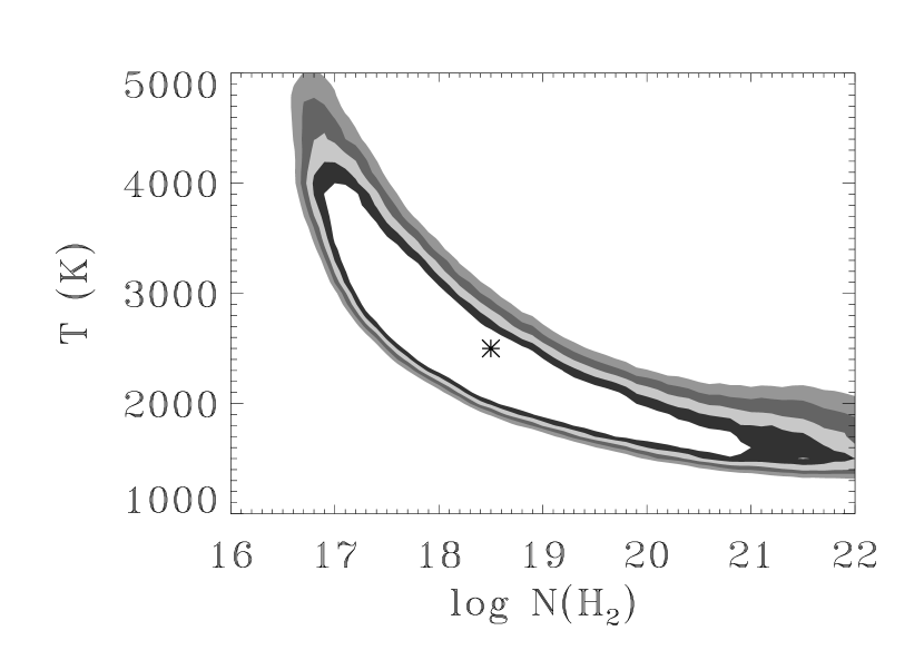
Figure 9: $1-5\sigma$ confidence contours calculated from $\Delta\chi^{2}_{\nu,H2}$ for fits to the individual H₂ line fluxes for the thick disk model (see §3). The star indicates the position of the model with $T=2500$ K and $\log N$(H₂)=18.5 (see §6).

We calculate the relative flux of each transition within a single progression, given an H₂ excitation temperature and column density of the slab, and a separate flux normalization factor for each progression. Models are calculated for temperatures in the range $T=$1000–5500 K, sampled at 100 K intervals, and column densities (in cgs units) of $\log N($H₂)=15–23, sampled at 0.1 dex intervals. $N$(H₂) and $T$ are then determined by fitting simultaneously the relative line fluxes for 19 observed progressions. Five lines are not used because they are blended, and one line is not used because it is anomalously weak due to C II wind absorption (see Paper I). The FUSE lines, observed six weeks after the STIS observations, are not used in building these models due to the potential problems with flux variability and cross-calibration between STIS and FUSE. The fits have 21 variables: 19 normalization factors, $N($H${}_{2})$, and $T$. In typical models, 46 of the 140 H₂ line fluxes are sensitive to H₂ line opacity, and hence $N($H₂) and $T$. The other 94 lines, which have only a weak dependence on $N($H₂) and $T$, determine the 19 normalization factors. We calculate $\chi^{2}_{\rm H2}$ for only the 46 lines which depend on $N($H₂) and $T$. Confidence contours of $1-5\sigma$, calculated from values of $\Delta\chi^{2}_{\nu,{\rm H2}}$ for 44 degrees of freedom, are shown in Figure 9, with a minimum $\chi^{2}_{\nu,{\rm H2}}=2.22$ at $\log N($H${}_{2})=17.9$ and $T=2600$ K.

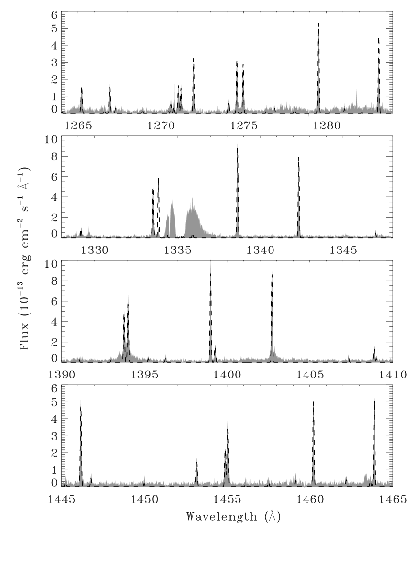
Figure 10: Selected regions of the HST/STIS spectrum of TW Hya. The narrow features are all H₂ lines. The dashed lines show our model fit to the H₂ emission. The line at 1333.8 Å is supressed by C II in the wind of TW Hya, which places the H₂ interior to the wind.

Based on this analysis, and additional constraints provided by the Ly$\alpha$ profile analysis described in §4, we ultimately decide a thick disk model with $T=2500$ K and $\log N$(H${}_{2})=18.5$ is our best model, which we adopt for the analysis (see §6.1). Figure 10 compares the observed spectrum compared with a synthetic spectrum computed from this model. The adopted model correctly predicts the fluxes of all strong H₂ lines. Only one observed line flux differs significantly from the model flux. The model predicts a flux of $46\times 10^{-15}$ erg cm^-2 s^-1 in the 0-4 R(1) transition at 1333.797 Å. The measured flux in this line, $(7.9\pm 0.7)\times 10^{-15}$ erg cm^-2 s^-1, is significantly reduced by C II wind absorption, as discussed in Paper I. The 0-3 P(3) transition at 1283.16 Å, with a measured flux of $28.0\times 10^{-15}$ erg cm^-2 s^-1, is moderately weaker than the model flux of $34.8\times 0^{-15}$ erg cm^-2 s^-1, possibly because of H₂ absorption in the 2-2 R(15) transition, centered 8 km s^-1 from the 0-3 P(3) transition. Table 3 lists predicted fluxes for Lyman-band H₂ transitions in the FUSE bandpass. Future measurements of flux in these transitions would provide a good test for our model. Lines at $\lambda<1200$ provide particularly good constraints since they are transitions to very low energy levels, and as a result have large opacities.

Neither this model nor the alternative models presented in §5 rigorously simulate a disk geometry. Because the structure of disks is uncertain near the truncation radii, we do not have an accurate picture of the geometry of the H₂ emission region. Without this a priori knowledge, the thick disk geometry described here is not clearly better or worse than any other oversimplified geometry that we might assume. In §5, we will show that the temperature of the molecular region is relatively insensitive to geometry, and we will rule out certain geometries that cannot sufficiently explain the observed H₂ spectrum. Since our models make as few assumptions as possible, the primary result of this paper, the temperature of the H2 gas, may apply to a wide range of other morphologies.

4 RECONSTRUCTED Ly$\alpha$ PROFILE

In this section, we reconstruct the Ly$\alpha$ profile seen by the warm H₂ gas at the 18 pumping wavelengths between 1212–1220 Å. Fluorescent H₂ emission occurs because certain Lyman-band transitions, with lower levels $1-2$ eV above the ground state, have wavelength coincidences with the broad Ly$\alpha$ profile. The emission in each progression depends on the Ly$\alpha$ flux at the pumping wavelength of the fluorescent transition, the upward transition probability, the opacity in the pumping transition, and the filling factor of H₂ as seen from the source of the Ly$\alpha$ emission. We reconstruct the incident Ly$\alpha$ profile following a procedure similar to that used by Wood et al. (2002) to analyze fluorescent H₂ emission in the HST/STIS spectrum of Mira B. A comparison of the reconstructed and observed Ly$\alpha$ profiles provide another constraint on the values of $T$ and $N$(H₂), that is independent of the constraints provided by the analysis presented in §3. The analysis in §3 relied upon using the H₂ flux ratios within each fluorescence progression to constrain $T$ and $N($H${}_{2})$, whereas the Ly$\alpha$ profile reconstruction analysis presented in this section relies only on the total flux from each upper level.

We calculate the optical depth in each H₂ pumping transition by assuming that the absorption line profiles in the model slab are Voigt functions with a Doppler $b$ parameter, which depends on an assumed temperature, and a damping parameter $a$ from Abgrall et al. (1993). The total Ly$\alpha$ flux, $F_{abs}$, absorbed by a given lower level is then

$$F_{abs}=\eta\times F_{inc}\times\int_{\lambda}1-e^{-\tau_{\lambda}[T,N(H_{2})]}{\rm d}\lambda$$ (3)

where $F_{inc}$ is the incident Ly$\alpha$ flux per unit wavelength and $\int_{\lambda}1-\exp^{-\tau_{\lambda}[T,N(H_{2})]}$d$\lambda$ is the equivalent width of the absorption profile within the slab (see EQW_slab in Table 2). Not every absorbed Ly$\alpha$ photon produces an observed H₂ photon. For the most highly excited states, the dissociation probability ($P_{dis}$ in Table 2) can be as large as 42%. Some fraction ($R_{unseen}$ in Table 2) of the emitted photons will be in spectral lines that we did not observe due to line blends, noisy data, or insufficient wavelength coverage. In our plane-parallel slab model, an emerging photon travelling normal to the slab sees a smaller optical depth than a photon travelling nearly parallel to the slab. As a result, the emitted flux in these models is largest for angles normal to the slab.

For comparison with the observed Ly$\alpha$ profile, we compute reconstructed Ly-alpha profiles for the same grid of $T$ and $N($H₂) values used in §3. Model fluxes at 8 pumping transitions, all on the red wing of the Ly$\alpha$ line, are fitted to the observed profile. The observed Ly$\alpha$ flux at other pumping wavelengths is corrupted by interstellar or wind absorption. Two progressions, 3-3 R(2) at 1217.031 Å and 3-3 P(1) at 1217.038 Å, are not included in the fit because their absorption profiles overlap, complicating the analysis. Photoexcitation of H₂ by C III emission via the transition 3-2 P(4) at 1174.923 Å may also add flux to the progression pumped by 3-3 R(2). We judge the suitability of a model using a modified $\chi^{2}$ analysis to measure the scatter in the red wing of the reconstructed profile. Errors in the Ly$\alpha$ line wing tend to be multiplicative, rather than additive, so we define $\chi^{2}_{Ly\alpha}$

$$\chi^{2}_{Ly\alpha}=\sum(\frac{F_{obs}}{\sigma_{obs}}\log\frac{F_{obs}}{F_{mod}})^{2}$$ (4)

based on standard error propagation techniques from Bevington (1969). Using this formula, an overestimate and an underestimate of the reconstructed Ly$\alpha$ profile by a factor of 10 will result in the same contribution to $\chi^{2}_{Ly\alpha}$.

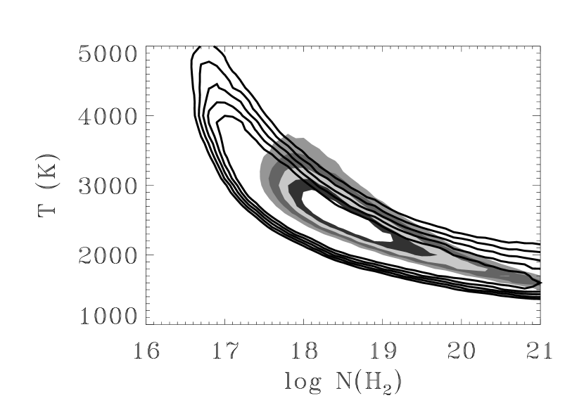
Figure 11: $1-5\sigma$ confidence contours calculate from $\Delta\chi^{2}_{\nu,Ly\alpha}$ (shaded regions) for our fit of the reconstructed Ly$\alpha$ profile to the red wing of the observed Ly$\alpha$ profile, compared with $1-5\sigma$ confidence contours (solid lines) for fits to the observed H₂ fluxes.

Figure 11 shows confidence contours of $1-5\sigma$ calculated from $\Delta\chi^{2}_{\nu,Ly\alpha}$ for fits to the observed Ly$\alpha$ profile, with 5 degrees of freedom. In the thick disk geometry, a minimum $\chi^{2}_{\nu,Ly\alpha}=2.31$ is obtained when comparing the reconstructed and observed Ly$\alpha$ profiles for $\log N$(H₂)=18.5, $T=2500$ K, and $\eta=0.25$. The top panel of Fig. 12 shows that these parameters yield an excellent fit to the observed profile. These parameters also reproduce the individual line fluxes well (see §3 and Fig. 9). Since the confidence contours calculated from the Ly$\alpha$ profile analysis place a more stringent constraint on the temperature and column density than do the contours from fitting individual line fluxes (see Fig. 11), we choose on the values of $T$ and $N$(H₂) quoted above as our best estimates of these parameters. The model dependent quantities listed in Table 2 are all calculated using these parameters.

More than 500 other possible upward transitions in the Lyman-band have wavelengths between 1210–1220 Å. Fluorescent emission in lines from these weaker progressions is below our detection limit. Table 4 identifies undetected progressions with the largest predicted emission line fluxes. The table includes our observational flux limit $F_{max}$ on the strongest line in the progression at wavelength $\lambda_{max}$. For any H₂ line that is not detected and does not appear in Table 4, we place an upper flux limit of $5\times 10^{-15}$ erg cm^-2 s^-1. We then use these upper limits to calculate an upper limit of Ly$\alpha$ at the pumping wavelength to test the self-consistency of our model.

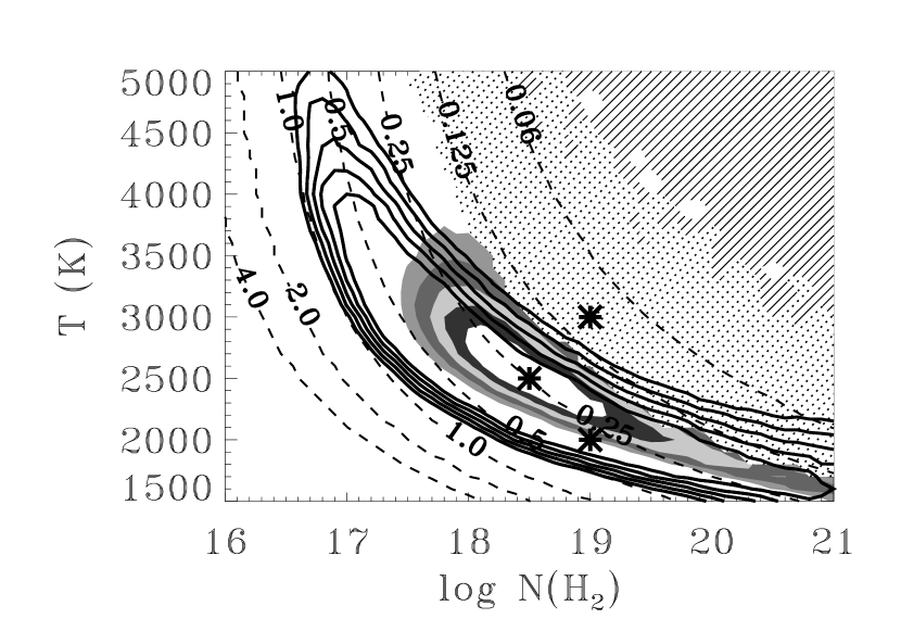
Figure 13: Similar contours as in Figure 11. The dots indicate the parameter space that we rule out because those parameters predict that lines pumped by 7-4 P(5) should be observed, and the diagonal lines indicate the parameter space ruled out because many additional other progressions should be observed but are not detected. Filling factor contours (dashed lines) of 0.125–4.0 are also shown. A filling factor above 1 is unphysical. The three models with reconstructed Ly$\alpha$ profiles in Fig. 13 are shown as asterisks.

Figure 12 shows three examples of reconstructed Ly$\alpha$ profiles (circles), with upper limits to the Ly$\alpha$ flux at certain wavelengths calculated from upper limits of lines in the undetected progressions (arrows), as described above. The top panel shows the Ly$\alpha$ profile constructed using the parameters for our adopted model [$\log N($H₂)=18.5, $T=2500$ K, and $\eta=0.25$]. This profile is smooth, and its wings correspond well with the wings of the observed Ly$\alpha$ profile. The upper limits on the flux of Ly$\alpha$ calculated from undetected progressions are all consistent with the Ly$\alpha$ profile reconstructed from observed progressions. The middle panel shows a Ly$\alpha$ profile calculated from a model with $\log N($H₂)=19.0, $T=2000$ K, and $\eta=0.4$, which is inconsistent with the data because of a large amount of scatter in the red wing of the reconstructed Ly$\alpha$ profile. The bottom plot shows a Ly$\alpha$ profile calculated from a model with $\log N($H₂)=19.0, $T=3000$ K, and $\eta=0.2$, which is also inconsistent with the data because at 1214.421 Å the predicted Ly$\alpha$ emission required to pump the $\hbox{$v^{\prime}$}=7,\hbox{$J^{\prime}$}=4$ level is significantly below the observationally constrained flux at 1214.465 Å. Figure 13 is a reproduction of Figure 11, with dotted and diagonal lines added to show the region of parameter space that are excluded because upper limits on H₂ emission would imply a Ly$\alpha$ pumping flux significantly lower than the nearby Ly$\alpha$ pumping flux for a progression of observed H₂ lines. Parameter space constraints are shown separately for upper limits on progressions pumped via 7-4 P(5) at 1214.421 Å alone (dots) and via a set of others upward transitions (diagonal lines). The parameter space with $\eta>1$ (dashed lines in Fig. 13) are unphysical models, and are also ruled out.

The three reconstructed Ly$\alpha$ profiles shown in Figure 12 are roughly similar to each other and to most other Ly$\alpha$ profiles that we have reconstructed for other values of $T$ and $N$(H₂). Each profile shows a clear depression near Ly$\alpha$ line center that is not nearly as wide as the observed H I absorption. Figure 14 demonstrates that the absorption feature in the reconstructed Ly$\alpha$ profile can be characterized by a column density $\log N($H I$)\approx 18.7$ centered 90 km s^-1 shortward of line center. This H I between the source of Ly$\alpha$ emissio and the warm H₂ could be in the base of a wind or at the disk surface. Alternatively, the shape of the Ly$\alpha$ profile could be an intrinsic self-reversal, in which case the intervening H I need not exist. The blue side of the reconstructed Ly$\alpha$ profile is enhanced relative to the observed Ly$\alpha$ profile, because wind absorption in our line of sight to the star attenuates the intrinsic emission. This result supports our conclusion from Paper I that, in our line of sight, the H₂ must be photoexcited interior to most of the wind that we detect.

5 ALTERNATIVE GEOMETRIES

In §3 and §4, we described in detail results for a dust-free thick disk geometry, which may not represent the true morphology of warm gas around the star. In this section, we explore the same parameter space for a thin disk geometry, shown schematically in Figure 8, and a cloud geometry, which approximates H₂ emission from a cloud in our line of sight to the star.

The computed H₂ fluxes depend on the angle at which Ly$\alpha$ photons enter the disk, the exit angle of H₂ photons, and the extinction either within the disk or in the ISM. Figures 15 and 16 and Table 5 present the best-fit parameters from fitting the H₂ line opacities for each of three geometries as a function of the exit angle of H₂ and extinction within the disk. In general, while changes in the geometry of the system can mildly change some results, the calculated temperature of the warm gas depends primarily upon the molecular physics and not on the geometry. The calculated column density of H₂ and its physical interpretation, however, do depend on the assumed geometry. In what follows, the column density represents the amount of H₂ in a line of sight normal to the disk surface, regardless of the path length the Ly$\alpha$ photons traverse through the disk.

5.1 Thin Disk Geometry

A thin disk (see Fig. 8) is characterized here as a disk for which the filling factor of H₂ around the Ly$\alpha$ source is dominated by the surface layers of the disk, rather than by the inner edge of the disk. We approximate this geometry with a model in which the incident Ly$\alpha$ photons enter a plane-parallel slab at a large angle with respect to the disk normal and are reprocessed into H₂ photons that emerge normal to the slab. Because Ly$\alpha$ photons enter the slab at a large angle, the radiation is reprocessed into H₂ emission at a shallow depth, and the emerging H₂ photons see a smaller optical depth in this geometry than in the thick disk geometry. For the thin disk geometry, with incident photons entering the disk at $\theta=80^{\circ}$, the best-fit parameters are $T=2500$ K, $N($H₂)=20.0, but with an unacceptable $\chi_{\nu,H2}^{2}=7.9$, for fits to H₂ line fluxes. For fits of the reconstructed to the observed Ly$\alpha$ line, the confidence contours move to smaller column densities by a factor of $\sin\theta$. As the angle of incidence asymptotically approaches 90^∘, the Ly$\alpha$ photons are converted into H₂ photons close to the disk surface. Since the optical depth traversed by the emitted H₂ photons is negligible, the relative line fluxes with each progression differ from predicted branching ratios only because of extinction, which we find to be unlikely (see §2.2 and §5.3).

5.2 Cloud Geometry

We next consider a geometry in which the H₂ is located between us and the source of Ly$\alpha$ photons. In this geometry, the escaping photons must travel through a greater optical depth of H₂ than they would in the other geometries that we considered. As a result, the acceptable contours for fits to H₂ line fluxes move towards smaller column densities relative to the thick or thin disk geometries. Even in this very different geometry, the confidence contours for the Ly$\alpha$ reconstruction fitting do not move much in parameter space, and they restrict the gas temperature to 2000–3000 K. The best-fit parameters in fitting H₂ fluxes for this geometry are $T=2600$ K, $N($H₂)=17.8, with $\chi^{2}_{\nu,H2}=2.8$. The transmission geometry is probably not realistic for TW Hya, but it can be used to set limits on the column of warm H₂ between us and the source of Ly$\alpha$ emission. The absence of any observed H₂ absorption in the Ly$\alpha$ profile (Fig. 3) allows us to place a limit on the column density in this level of $\log N(\hbox{$v^{\prime\prime}$}=2,\hbox{$J^{\prime\prime}$}=1)<14.4$ and a total column density of warm H₂ of $\log N($H${}_{2})<16.1$. Thus, the detected H₂ fluorescence does not occur in our line of sight to TW Hya.

5.3 Dust Extinction in the Disk and the ISM

In §2, we presented evidence that the dust extinction along our line of sight to the Ly$\alpha$ emission source is negligible. Extinction of H₂ emission could occur within the disk if dust is mixed with the warm gas, although Calvet et al. (2002) found that small dust grains are underabundant within 5 AU of the star. We assume an interstellar extinction law from Cardelli et al. (1989), for grains typical of the interstellar medium ($R_{V}=3.09$).

For each H₂ progression, the average depth $d_{abs}$ of the initial Ly$\alpha$ absorption depends on the opacity of the lower level of H₂ (see Fig. 17 and Table 2). If a Ly$\alpha$ photon is, on average, absorbed close to the disk surface, then the H₂ lines excited by that photon will not be significantly attenuated by any disk extinction. Thus, the extinction varies for the different progressions. In Figure 16, $A_{V}$ represents the extinction through half of the slab (not the extinction through the entire slab or the extinction from the star to the observer), which is equal to the largest possible average extinction of H₂ emission when Ly$\alpha$ photons are absorbed uniformly throughout the slab. Disk extinction attenuates both the incident Ly$\alpha$ emission and the outgoing H₂ emission, but not the observed Ly$\alpha$ emission, and thus increases the already large filling factor. In the context of our model, significant disk extinction can be ruled out because the computed filling factors would be much larger than unity.

Interstellar extinction affects the fluxes smoothly across the wavelength region, and does not significantly impact the derived filling factor because it attenuates both the observed Ly$\alpha$ emission and the H₂ emission. If we consider only extinction and ignore opacity in the H₂ lines, then from fitting H₂ line fluxes we obtain a minimum $\chi^{2}_{\nu,H2}=6.06$ at $A_{V}$=1.3, which is significantly larger than the $\chi^{2}_{\nu,H2}$ for the best-fitting models.

5.4 Adoption of the Thick Disk Geometry

Based on these results, and the results presented in Figs. 15-16 and Table 5, we adopt the thick disk geometry (Geometry 2 in Table 5) as the preferred geometry to describe the H₂ emission. The thick disk geometry is physically plausible and produces reasonably good fits with self-consistent results, although certain other geometries can produce lower values of $\chi^{2}$ in fits to H₂ fluxes or in the Ly$\alpha$ fits. Some of those geometries (e.g., Geomteries 7 and 8 from Table 5) represent morphologies that are difficult to reconcile with our previous conclusion that the H₂ emission occurs in a disk. In other geometries (e.g., Geometries 1 and 11 from Table 5), contours from the H₂ flux fitting do not overlap with the contours from the Ly$\alpha$ fitting as well as they do for the thick disk geometry, i.e. the joint probability is lower (see Fig. 11).

We caution the reader that the thick disk geometry is best only in the context of our restricted set of models. Warm H₂ in the TW Hya star-disk system could in principle have a morphology not considered here.

6 DISCUSSION

6.1 Synthesizing the H₂ and Ly$\alpha$ modelling results

Figures 11 and 13, and Table 5, compare results from our analysis of individual H₂ line fluxes with our results from the Ly$\alpha$ profile reconstruction. Based on the overlap region of acceptable models for both the individual H₂ line fluxes and the reconstructed Ly$\alpha$ profile, we conclude that a column density of $\log N($H${}_{2})=18.5^{+1.2}_{-0.8}$ is heated to a temperature of $2500^{+700}_{-500}$ K, with a filling factor of $\eta=0.25\pm 0.08$ around TW Hya ($2\sigma$ error bars). Table 2 lists the percentage $P_{dis}$ of H₂ that dissociates from the upper level, the H₂ dissociation rate in terms of mass ($M_{dis}$), and the total flux for each progression ($F_{mod}$) for our best-fit model of $\log N($H${}_{2})=18.5$ and $T=2500$ K. The notion of a single temperature is a simplistic assumption, but it is sufficient to reproduce our data. The temperature derived here is warmer than the $\sim 1100-1300$ K temperatures seen in the fundamental CO emission by Najita et al. (2003).

The mass column corresponding to $\log N($H₂)=18.5 is $10^{-5}$ g cm^-2, which is about $10^{-7}$ times smaller than the mass column predicted to be within 1 AU by D’Alessio et al. (1999). This suggests that H₂ fluorescence probably occurs in a very shallow surface layer of the disk, which could be a warm, extended disk atmosphere. The Ly$\alpha$ fluorescence process cannot be used to detect cold H₂, which most likely represents the bulk of the mass in the disk.

In our models, we assume that H₂ gas is thermalized, so that relative level populations depend only on temperature. This is reasonable because the gas density at the disk surface should be between $n_{H}=10^{6}-10^{8}$ cm^-3 (Gomez & D’Alessio, 2000), which is far larger than the critical density of $n_{H}$=$10^{4}$ cm^-3 at which collisions typically dominate over quadrupole radiative de-excitation. Below the critical density, collisions cannot repopulate excited H₂ levels as fast as they radiatively deexcite. Fluorescent progressions pumped out of higher energy states would be weaker than expected from our thermal models, generating scatter that we do not see in our reconstructed Ly$\alpha$ profile. This conclusion confirms the assumption of thermally excited H₂ gas used by Black & van Dishoeck (1987) and Burton et al. (1990) to model H₂ fluorescence.

6.1.1 Filling factor of H₂ around the Ly$\alpha$ source

Figure 13 shows that the filling factor of the H₂ around the Ly$\alpha$ emitting region is $\eta=0.25\pm 0.08$. This factor represents the solid angle of the sky subtended by H₂ as seen from the source of Ly$\alpha$ photons near TW Hya, although other geometrical effects may contribute. Neutral hydrogen mixed with the warm H₂ could scatter Ly$\alpha$ photons, increasing the effective path length of the Ly$\alpha$ photons and thereby reducing the calculated filling factor. Any directional dependence of the Ly$\alpha$ emission, and the percentage of Ly$\alpha$ emission visible to us versus the percentage visible to the warm H₂, will also affect the calculated filling factor. A total of 1-2% of the intrinsic Ly$\alpha$ emission is reprocessed into H₂ emission (see Table 6 and §4), which places a lower limit of 0.01 on the filling factor.

For any flared disk geometry, the filling factor can be converted into a disk height by comparing the surface areas of a cylinder and a sphere. For $\eta=0.25$, the implied geometrical disk height from the midplane to the surface at distance $R$ from the center of the star is H=$0.25(\frac{R}{1AU})$ AU, compared with predicted disk heights from (D’Alessio, 2001) of about 0.15 AU at a distance of 1 AU from the star.

6.1.2 Relationship between UV and IR H₂ Emission

Emission in the 1-0 S(1) rovibrational transition at 2.1218 $\mu$m has been detected from 4 T Tauri stars (Bary et al., 2003). The narrow width and absence of any velocity shift with respect to the stars suggests a disk origin of this emission. The flux in this line from an optically thin emission region

$$F=\frac{N(1,3)\pi r^{2}A_{ul}}{4\pi d^{2}}\frac{hc}{\lambda},$$ (5)

where $N(1,3)$ is the H₂ column density of the disk in the $\hbox{$v^{\prime\prime}$}=1,\hbox{$J^{\prime\prime}$}=3$ level, $\pi r^{2}$ is the projected surface area of the emission region, and $A_{ul}=3.47\times 10^{-7}$ s^-1. If the 1-0 S(1) line flux of $1\times 10^{-15}$ erg cm^-2 s^-1 measured by Weintraub et al. (2000) comes from a heated disk surface layer with N(H2)=18.5 and T=2500 K, then the 1-0 S(1) emission must extend out to at least 5 AU for a face-on disk. This corresponds to an angular extent of $\pm 0\farcs 1$, which could have been resolved in our HST observations, but was not. Thus, it seems likely that at least some of the 1-0 S(1) emission comes from H₂ gas that is not fluoresced by Ly$\alpha$. Some of the emission in the 1-0 S(1) line may be produced deeper in the disk or farther from the star, as a result of X-ray ionization and subsequent collisional excitation of H₂ by non-thermal electrons (Weintraub et al., 2000).

6.1.3 H₂ Dissociation Rate

From the flux in observed transitions, we calculate a dissociation rate of $9.8\times 10^{-11}$ $M_{\odot}$ yr^-1 for H₂ in the disk. Forward modelling of undetected Lyman and Werner-band transitions excited by Ly$\alpha$ photons increases the calculated dissociation rate to $1.6\times 10^{-10}$ $M_{\odot}$ yr^-1. Depending on the timescale for collisional de-excitation of H₂, the actual dissociation rate could be much higher due to multiple pumping [pumping from lower rovibrational levels of H₂ that are populated by the initial pump and subsequent fluorescence – see Shull (1978) for details], which can populate highly excited rovibrational levels in the B electronic state that have dissociation probabilities as high as 50%.

The H₂ dissociation rate we estimate is within a factor of 10 of TW Hya’s mass accretion rate (see §2.1), meaning that the dissociation provided by Ly$\alpha$ fluorescence may be an important process in the accretion of hydrogen onto the star. The neutral H released by dissociation will cause the incident Ly$\alpha$ to scatter, increasing the probability of absorption in the pumping transitions and therefore decreasing the required filling factor. The neutral H could also be sufficiently optically thick to produce the self-reversal of the Ly$\alpha$ profile that irradiates the disk (see Fig. 14).

6.2 FUV radiation field

The FUV radiation field incident on the accretion disk can significantly affect the chemistry and temperature structure of the disk. In Table 6 we list the flux for spectral features in the FUV spectrum of TW Hya. The observed Ly$\alpha$ line contributes 67% of the observed FUV flux of $6.5\times 10^{-11}$ ergs cm^-2 s^-1 between 1170–1700 Å. From the reconstructed Ly$\alpha$ profile, we infer an intrinsic flux of $8-16\times 10^{-11}$ ergs cm^-2 s^-1, depending on the correction for the central absorption. With this correction, Ly$\alpha$ emission contributes 80–90% of the FUV flux of TW Hya, of which 1-2% is reprocessed into H₂ emission. The continuum accounts for about $6\times 10^{-12}$ ergs cm^-2 s^-1, or about 4% of the total emission, including the estimated intrinsic Ly$\alpha$ flux. The remaining flux occurs in other emission lines such as the C IV 1550 Å doublet. The UV flux below 1170 Å measured by FUSE adds at most 2% additional flux to the strength of the radiation field. The UV radiation between 1700–2000 Å may add to the radiation field, primarily due to emission in lines such as Si II] $\lambda$1817 and C III] $\lambda$1909, but will have little effect on the excitation of molecules and atoms in the disk. The estimated total emission after including Ly$\alpha$ flux that is not observable is approximately $10^{-3}$ $L_{\odot}$, assuming isotropic emission and a distance of 56 pc.

The properties of the disk, both in the PDR-like disk atmosphere and in the cooler outer regions, will be partially controlled by the Ly$\alpha$ emission, as evidenced by the fluorescent H₂ emission. Not only does Ly$\alpha$ dominate the FUV flux of TW Hya, but it can also scatter off neutral H towards the interior of the disk, allowing it to penetrate the disk further than continuum UV radiation. Ly$\alpha$ can dissociate molecules such as H₂ and H₂O, and can ionize Si and C. Bergin et al. (2003) explain that the enhancement of CN relative to HCN occurs in disks because Ly$\alpha$ radiation can photodissociate HCN, whereas CN can be dissociated only by radiation with $\lambda<1150$ Å.

6.3 Heating mechanisms

We have found evidence for a warm surface layer of H₂ on the disk around TW Hya. From the lack of spatial extent in the STIS echelle cross-dispersion direction, the heated surface is located within 2 AU of the star. Models of dust in disks of CTTSs typically predict $T\approx 1000$ K only within 0.1 AU of the star (D’Alessio et al., 2001; Chiang & Goldreich, 1997). The FUV radiation field at 1 AU from the star is approximately $10^{7}$ $G_{0}$, where the Habing field $G_{0}=1.6\times 10^{-3}$ erg cm^-2 s^-1 (the local interstellar field is 1.7 $G_{0}$), which is stronger than the FUV radiation field incident upon most PDRs ($10^{3}-10^{6}$ $G_{0}$). Hollenbach, Yorke & Johnstone (2000) predicted from models of photo-dissociation regions that a warm atmosphere-like structure, heated by UV radiation, should surround the inner regions of a disk, with a temperature between 500 and 3000 K.

Because of the absence of micron-sized dust grains within 5 AU of TW Hya (Calvet et al., 2002), a large percentage of the FUV radiation may be deposited into the gas. In their analysis of the H₂ fluorescence from Mira B, Wood et al. (2002) found that the temperature increases sharply with radius from the UV source, and that the Ly$\alpha$ fluorescence process is a significant heating source for the gas. The energy deposited into the warm gas near TW Hya due to Ly$\alpha$ photoexcitation and subsequent fluorescence is $1.4\times 10^{29}$ erg s^-1, which corresponds to roughly 0.01 eV s^-1 per molecule of H₂. The strong X-ray luminosity of TW Hya, $L_{X}=3.6\times 10^{-4}~{}L_{\odot}$ between 0.45–6.0 keV (Kastner et al., 2002), could heat the disk surfaces by an additional 500 K (Igea & Glassgold, 1999; Glassgold & Najita, 2001; Fromang et al., 2002) by ionizing atoms to produce a large reservoir of energetic non-thermal electrons (e.g., Maloney et al., 1996; Yan & Dalgarno, 1997). X-rays can also penetrate deeper into the gas than UV radiation and, consequently, may heat gas deeper in the disk than the UV radiation.

Certain observed fluorescence progressions are pumped from lower rovibrational levels with large energies, such as $\hbox{$v^{\prime\prime}$}=3,\hbox{$J^{\prime\prime}$}=25$ ($E^{\prime\prime}=4.2$ eV) and $\hbox{$v^{\prime\prime}$}=5,\hbox{$J^{\prime\prime}$}=18$ ($E^{\prime\prime}=3.8$ eV). The measured flux in these progressions, comibed with the observed flux at the pumping wavelengths, requires that of order 1% of the H₂ resides in these levels. This population is too large to be thermally populated at any reasonable temperature for the H₂ gas. Therefore, non-thermal processes must be populating these levels. Although the fluorescence process can populate high vibrational levels in the ground electronic state, fluorescence cannot directly populate high rotational levels, and no direct paths exist to the levels $\hbox{$v^{\prime\prime}$}=3,\hbox{$J^{\prime\prime}$}=25$ and $\hbox{$v^{\prime\prime}$}=5,\hbox{$J^{\prime\prime}$}=18$. H₂ can form in highly excited states (Kokoouline, Greene, & Esry, 2001; Strasser et al., 2001) via dissociative recombination of H${}_{3}^{+}$. Given a dense medium and a large ionizing flux, then H${}_{2}^{+}$ may be present in large enough quantities to react with H₂ to produce H${}_{3}^{+}$ in highly excited states. More attempts to detect H${}_{3}^{+}$ would be useful.

7 SUMMARY

We have modeled a plane-parallel slab of warm H₂ (see Fig. 1), which represents the surface of a protoplanetary disk irradiated by UV flux from the star. Our analysis of the ultraviolet spectrum of TW Hya obtained with the STIS instrument on HST and with FUSE leads to the following conclusions:

1. The FUV continuum rises shortward of 1700 Å, which is indicative of an H₂ dissociation continuum, although it could also be produced by H₂ fluorescence due to FUV continuum pumping or an additional accretion or activity component. The FUV continuum is not well explained by simple models of a pure hydrogen slab, which are commonly invoked to analyze the excess NUV continuum.

2. The extinction towards TW Hya is negligible, based on the hydrogen column density in our line of sight and assuming an interstellar gas-to-dust ratio.

3. Self-absorption of Lyman-band transitions involving low excitation energy levels weakens the flux in these lines. We model this effect by simulating Ly$\alpha$ emission entering a plane-parallel atmosphere and pumping the H₂.

4. Using the observed H₂ fluxes and our fluorescence models, we reconstruct the Ly$\alpha$ line profile incident upon the warm molecular layer and compare it to the observed Ly$\alpha$ profile, for a range of assumed temperatures and column densities. Undetected progressions rule out a large region of parameter space in this model. The reconstructed Ly$\alpha$ profile is similar to the observed profile in the wings, but shows a much narrower absorption feature than is observed. This narrow absorption component in the reconstructed profile could be a self-reversal or a component of the wind between the source of Ly$\alpha$ emission and the warm molecular region.

5. Our models indicate that a molecular layer with a kinetic temperature of $2500^{+700}_{-500}$ K and a column density of $\log N$(H${}_{2})=18.5^{+1.2}_{-0.8}$ ($2\sigma$ error bars) absorbs Ly$\alpha$ radiation in the surface layer and inner edge of the disk within 2 AU of the central star. The Ly$\alpha$ pumping leads to a small H₂ dissociation rate and does not cause significant disk dissipation. The filling factor of the warm H₂ around TW Hya is $\eta=0.25\pm 0.08$, although significant uncertainties in the geometry of the fluorescent H₂ weaken our confidence in the large filling factor.

6. The warm H₂ most likely resides in a warm surface layer of the disk. This surface layer may be analgous to a classic PDR, although in this case the FUV radiation field is dominated by emission lines rather than a continuum. In particular, Ly$\alpha$ comprises about 85% of the FUV radiation field below 2000 Å, and it controls the excitation and ionization of the disk surface.

7. Some of the observed H₂ lines are pumped from high rotational levels that cannot be excited thermally or by fluorescence. Formation of rotationally excited H₂ by reactions with H${}_{3}^{+}$ may explain these emission lines.

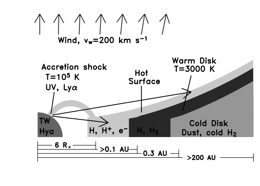
Figure 1: A schematic diagram of our model of TW Hya and its disk (not to scale). FUV radiation, primarily Ly$\alpha$, is produced at the accretion shock and heats the disk. The warm H₂ is located in surface layers of the disk within 2 AU of the star. The hot surface of the disk, composed of atoms and ions, probably extends inwards to about $6R_{*}$ (Johns-Krull & Valenti, 2001b), where it is truncated by the stellar magnetosphere.

Figure 2: The solid line shows the observed spectrum of of TW Hya, after subtracting the template spectrum of V819 Tau. The dashed line shows the synthetic spectrum of a pure hydrogen slab fit to the observed Balmer jump and the Balmer lines. The pure hydrogen continuum accurately approximates the NUV continuum of TW Hya but significantly underestimates the FUV continuum. The rise of the FUV continuum shortward of 1700 Å is indicative of an H₂ dissociation continuum produced by collisions with energetic electrons, although it could also be produced by H₂ fluorescence due to FUV pumping or an additional accretion or activity component.

Figure 3: The Ly$\alpha$ emission from TW Hya is partially absorbed by H I in the line of sight to TW Hya. The interstellar and circumstellar media, centered at about 0 km s^-1, account for the red side of the absorption. The blue side of the absporption is produced by H I in the wind. The dashed line shows our best fit to the observed Ly$\alpha$ profile (solid line) using two Gaussian emission profiles to model the intrinsic Ly$\alpha$ line before the absorption, while the dotted and dashed-dotted lines assume different H I column densities that poorly fit the red side of the observed profile.

Figure 4: The transmission percentage across the observed Ly$\alpha$ profile (solid) for column densities $\log N$(H)$=19.75$ (dashed) and $\log N$(H)$=20.5$ (dotted), assuming no Doppler broadening. This assumption places a strong upper limit of $N($H I$<19.75$) towards TW Hya.

Figure 5: The O VI emission line from TW Hya (solid), as observed with the LiF1a detector on FUSE. We place a limit of $N($H₂)$<18$ in our line of sight towards TW Hya by comparing the observed emission with the simulated transmission percentage given the resolution of FUSE, through a medium of H₂ with $T=100$ K and $N($H${}_{2})$=17.5 (dashed) and $N($H${}_{2})$=19.0 (dotted). We would observe many H₂ absorption lines against the O VI emission from TW Hya for hotter excitation temperatures of H₂.

Figure 6: The NUV continuum (solid) is well fit by the accretion model (dashed) for $A_{V}=0.0$, but if $A_{V}=0.5$, the rise in the continuum below 2600 Å is not fit well.

Figure 7: For four different upper levels, we plot the normalized ratio of the observed de-excitations in each H₂ line divided by the respective branching ratio (circles). The squares show the fluxes prediced based on the optical depth in each lower level for our adopted model for $\log N($H${}_{2})=18.5$ and $T=2500$ K (see §5). The dotted and dashed lines show extinction curves for $A_{V}=0.5$ and $1.5$, respectively. Emission in an optically thin medium, with no intervening extinction, would result in ratios of 1.0. The apparent wavelength dependence results from the larger optical depth in those levels of H₂ which have lower excitation energies. The H₂ line fluxes from $v^{\prime}$=4, $J^{\prime}$=18 show no wavelength dependence because the observed lines all have lower levels with energies large enough that they are not populated.

Figure 8: Two plausible geometries for H₂ fluorescence in the surface layers of a protoplanetary disk. The Ly$\alpha$ enters the surface layer of H₂ at angle $\theta$ with respect to the normal and is reprocessed into H₂ emission, which escapes the disk at angle $\phi$.

Figure 12: Comparison of the observed (solid line) and calculated (circles) Ly$\alpha$ emission profiles, for models with (top) $\log N($H₂)=18.5, $T=2500$ K, and $\eta=0.25$ (middle) $\log N($H₂)=19.0 $T=2000$ K, and $\eta=0.41$; and (bottom) $\log N($H₂)=19.0 $T=3000$ K, and $\eta=0.20$. The arrows show upper limits to the calculated Ly$\alpha$ emission based on undetected H₂ progressions. The top plot is the best fit because of the least scatter in the red wing of Ly$\alpha$. The bottom model is unacceptable because several undetected progressions ($\hbox{$v^{\prime}$}=7,\hbox{$J^{\prime}$}=4$ pumped at 1214.4 Å and $\hbox{$v^{\prime}$}=5,\hbox{$J^{\prime}$}=20$ pumped at 1217.7 Å) imply upper limits of Ly$\alpha$ flux that are significantly lower than the flux reconstructed from nearby detected progressions.

Figure 14: The reconstructed Ly$\alpha$ profile at the wavelengths of the pumping transitions (diamonds) for $T=2500$ K, $\log N($H₂)=18.5, and $\eta=0.25$ corresponds well to a plausible Ly$\alpha$ profile (dashed line), constructed using a single Gaussian profile (dotted line) and an absorption feature of $\log N$(H I)$=18.7$ blueshifted 90 km s^-1 from line center.

Figure 15: Best-fit models to H₂ fluxes as a function of exit angle $\phi$ of H₂ photons, for the thick disk geometry (solid line), thin disk geometry (dashed line), and cloud geometry (dotted line).

Figure 16: Best-fit models to H₂ fluxes as a function of extinction within the H₂ slab, for the thick disk geometry (solid line), thin disk geometry (dashed line), and cloud geometry (dotted line). The extinction is for a progression in which the average Ly$\alpha$ photon is absorbed at the midplane of the slab.

Figure 17: The percent of the slab depth that a Ly$\alpha$ photon excites H₂ to two different upper levels (absorption depth $d_{abs}$ in Table 2), at two temperatures. As the column density and temperature of the slab increase, the optical depth in the lower levels increase, and a typical Ly$\alpha$ photon is reprocessed into H₂ at a shallower depth. This transition occurs at different column densities and temperatures for each progression, so that the reconstruction of the Ly$\alpha$ profile is sensitive to these parameters.

Table 1: LIST OF OBSERVATIONS

Star	Date	Instrument	Exposure Time	Grating	Aperture	Wavelength Range
TW Hya	2000 May 7	HST/STIS	260	G430L	$52\farcs\times 0\farcs 0.2$	2900-5700
	2000 May 7	HST/STIS	1675	E230M	$0\farcs 2\times 0\farcs 2$	2150–2950
	2000 May 7	HST/STIS	2300	E140M	$0\farcs 5\times 0\farcs 5$	1160–1700
	2000 Jun 22	FUSE	2081	1	$30\farcs\times 30\farcs$	900-1185
V819 Tau	2000 Aug 30	HST/STIS	360	G430L	$52\farcs\times 0\farcs 1$	2900-5700
	2000 Aug 31	HST/STIS	2325	E140M	$0\farcs 2\times 0\farcs 2$	2300-3100
	2000 Aug 30	HST/STIS	5700	E140M	$0\farcs 2\times 0\farcs 06$	1160–1700
1The FUSE instrument consists of several channels.

Table 2: H₂ PUMPING TRANSITIONS

Pump	$\lambda_{\rm calc}$	$E^{\prime\prime}$1	$A_{ul}^{2}$	$d_{abs}^{3}$	EQW${}_{slab}^{4}$	$R_{unseen}^{5}$	$P_{Dis}^{6}$	$P_{Dis,mod}^{7}$	$E_{dis}^{8}$	$M_{dis}^{9}$	F${}_{mod}^{10}$
	Å	eV	$10^{7}$ s-1	%	Å				eV
1-1 P(11)	1212.425	1.36	6.6	0.23	0.067	0.22	1.4(-5)	0.0	0.07	0.0	4.5
3-1 P(14)	1213.356	1.79	10.1	0.43	0.028	0.38	0.015	0.018	0.10	2.5	5.9
4-2 R(12)	1213.677	1.93	3.9	0.50	0.0092	0.30	0.050	0.067	0.15	4.4	2.7
3-1 R(15)	1214.465	1.95	10.0	0.37	0.044	0.16	0.031	0.039	0.02	15.6	17
4-3 P(5)	1214.781	1.65	5.5	0.43	0.030	0.25	1.9(-3)	2.0(-3)	0.11	0.0	11
4-3 R(6)	1214.995	1.72	3.0	0.50	0.0092	0.68	9.2(-3)	0.011	0.07	0.5	2.4
1-2 R(6)	1215.726	1.28	13.6	0.26	0.062	0.06	2.4(-6)	0.0	0.08	0.0	16
1-2 P(5)	1216.070	1.20	15.9	0.17	0.075	0.07	4.8(-7)	0.0	0.06	0.0	33
3-3 R(2)	1217.031	1.50	0.40	0.50	0.0015	0.45	2.8(-4)	0.0	0.05	0.0	2.4
3-3 P(1)	1217.038	1.48	1.7	0.50	0.0030	0.02	1.3(-4)	0.0	0.06	0.0	2.9
0-2 R(0)	1217.205	1.01	6.6	0.39	0.0413	0.09	4.3(-9)	0.0	0.07	0.0	38
4-0 P(19)	1217.410	2.21	4.4	0.47	0.014	0.47	0.42	0.51	0.18	64.0	5.1
0-2 R(1)	1217.643	1.02	7.8	0.21	0.0685	0.23	5.2(-9)	0.0	0.07	0.0	32
2-1 P(13)	1217.904	1.64	9.3	0.28	0.059	0.09	1.7(-3)	2.9(-3)	0.02	1.3	18
3-0 P(18)	1217.982	2.03	3.2	0.50	0.0068	0.57	0.19	0.21	0.11	9.5	1.9
2-1 R(14)	1218.521	1.79	7.6	0.43	0.028	0.42	5.9(-3)	6.5(-3)	0.09	0.6	3.6
0-2 R(2)	1219.089	1.05	8.2	0.29	0.0576	0.47	6.6(-9)	0.0	0.06	0.0	2.1
0-2 P(1)	1219.368	1.02	20.1	0.28	0.0599	0.30	3.9(-9)	0.0	0.06	0.0	1.2
0-5 P(18)	1548.146	3.79	19.1	0.50	0.0	0.36	1.1(-4)	0.0	0.11	0.0	3.0
1Lower energy level
2Radiative decay coefficient (Abgrall et al., 1993)
3Absorption depth of Ly$\alpha$ photon
4Equivalent width of absorption profile within slab
5Correction for unseen lines from upper level
6Dissociation probability from upper state per electronic excitation, $a(b)=a\times 10^{b}$.
7Dissociation probability from best-fit model.
8Average kinetic energy released due to H2 dissociation.
9H2 dissociation rate for best-fit model ($10^{-12}M_{\odot}$ yr-1).
10Ly$\alpha$ flux absorbed by lower level ($10^{-14}$ erg cm-2 s-1).

Table 3: STRONGEST PREDICTED LYMAN H₂ LINES IN THE FUSE BANDPASS

ID	$\lambda_{calc}$	$F_{mod}$	$F_{obs}$
4-0 R(3)	1053.973	1.1	$<3$
4-0 P(5)	1065.593	1.6	$<2$
4-1 R(3)	1101.889	2.4	$<10$
1-0 P(5)	1109.311	1.0	$<6$
3-1 P(1)	1113.877	1.4	$<6$
4-1 P(5)	1113.949	1.4	$<6$
1-1 R(3)	1148.701	5.0	$5.5(1.1)$
0-1 R(0)	1161.693	1.9	$13.1$(b)
1-1 P(5)	1161.814	6.2	$13.1$(b)
1-1 R(6)	1161.949	1.8	$13.1$(b)
0-1 R(1)	1162.170	2.4	$13.1$(b)
4-1 R(12)	1164.596	1.1	$<10$
2-0 P(13)	1165.834	1.0	$<6$
0-1 P(2)	1166.255	2.6	$<6$
0-1 P(3)	1169.751	2.5	$<10$
4-0 R(17)	1176.325	1.0	$<15$
3-1 R(12)	1179.472	1.3	$<10$
1-1 P(8)	1183.309	2.7	$<12$
2-1 R(11)	1185.224	2.8	$<12$
$F_{obs}$ refers to the observed fluxes and
$F_{mod}$ to the model fluxes in units of
$10^{-15}$ erg cm-2 s-1,$1\sigma$ error in ().
(b) indicates the line is blended with other H2 lines.

Table 4: UNDETECTED PROGRESSIONS

Pump	$\lambda_{\rm calc}$	$A_{ul}$	$E^{\prime\prime}$	$P_{Dis}$	$F_{\rm max}$	$\lambda_{\rm max}$	$\lambda_{ref}$	IDref
	Å	$10^{-7}$ s-1	eV		erg cm-2 s-1	Å	Å
1-1 R(12)	1212.543	4.6	1.49	5(-5)	$3\times 10^{-15}$	1578	1212.425	1-1 P(11)
7-4 P(5)	1214.421	2.8	2.07	0.19	$5\times 10^{-15}$	1582	1214.465	3-1 R(15)
5-3 P(8)	1218.575	6.6	1.89	0.04	$5\times 10^{-15}$	1608	1218.521	2-1 R(14)
5-0 P(20)	1217.716	5.4	2.39	0.48	$2\times 10^{-15}$	1223	1217.904	2-1 P(13)
2-2 P(8)	1219.154	10.8	1.46	7(-5)	$5\times 10^{-15}$	1579	1219.089	0-2 R(2)
2-2 R(9)	1219.101	12.9	1.56	2(-4)	$5\times 10^{-15}$	1572	1219.089	0-2 R(2)
5-3 R(9)	1219.106	5.4	1.99	0.085	$5\times 10^{-15}$	1601	1219.089	0-2 R(2)
3-3 R(1)	1215.541	0.46	1.48	2(-4)	$5\times 10^{-15}$	1596	1215.726	1-2 R(6)

Table 5: BEST-FIT PARAMETERS FOR ALTERNATE GEOMETRIES

Geometrya					Fit to H2 line opacities					Fit to Ly$\alpha$ profile
Number	Type	$\theta$	$\phi$	$A_{V}(D)$		$N($H${}_{2})$	$T$	$\eta^{b}$	$\chi^{2}_{\nu,H2}$		$N($H${}_{2})$	$T$	$\eta_{H2}$	$\chi^{2}_{\nu,Ly\alpha}$
1	Thick	0	89	0		17.0	2200	4.5	1.58		18.7	2400	0.29	0.9
2	Thick	0	77	0		17.9	2600	0.41	2.22		18.5	2500	0.25	2.3
3	Thick	0	77	0.5		17.5	2700	2.5	2.22		18.8	2800	0.23	9.5
4	Thick	0	77	1.0		17.6	2300	16	3.16		18.7	5300	0.09	18
5	Thick	0	77	1.5		23.0	1700	0.05	4.21		19.0	5300	0.09	17
6	Thick	0	43	0		19.1	2600	0.12	4.15		18.2	2700	0.23	3.0
7	Thick	0	0	0		19.5	2500	0.09	4.98		18.4	2600	0.21	3.3
8	Thin	80	89	0		16.6	2600	1.10	1.58		18.3	2200	0.31	1.1
9	Thin	80	77	0		18.7	2500	0.15	3.97		17.9	2400	0.27	0.8
10	Thin	80	43	0		20.2	2500	0.05	6.94		18.0	2400	0.23	0.8
11	Thin	80	0	0		20.0	2500	0.05	7.87		18.0	2400	0.22	0.8
12	Thin	80	0	0.5		19.2	2500	0.41	7.73		15.3	3300	$10^{5}$	29
13	Thin	80	0	1.0		17.9	1000	$10^{13}$	6.16		19.3	4700	0.03	33
14	Thin	80	0	1.5		15.9	4600	$10^{12}$	5.86		19.4	4900	0.03	34
15	Cloud	80	89	0		16.2	2800	8.2	1.96		18.5	2400	0.38	1.0
16	Cloud	80	77	0		17.3	2500	1.2	2.71		18.7	2400	0.26	0.5
17	Cloud	80	43	0		17.8	2500	0.52	2.92		18.7	2400	0.25	1.1
18	Cloud	80	0	0		17.8	2600	0.64	2.80		18.8	2300	0.33	0.9
19	Cloud	80	0	0.5		18.2	2000	12	2.74		18.8	2400	3.32	1.4
20	Cloud	80	0	1.0		18.1	1800	400	3.88		18.8	2500	40.4	1.9
21	Cloud	80	0	1.5		18.1	1400	104	6.07		18.8	2700	400	2.8
a$\theta$ and $\phi$ are defined in §3.2 and Fig. 8
b$\eta_{H2}$ calculated from Ly$\alpha$ reconstruction for parameters of best fit to H2 fluxes.

Table 6: FLUXES OF STRONG LINES

ID	$\lambda_{lab}$	Flux1
	Å	$10^{-12}$ erg cm-2 s-1
Total flux	1170–1700	$65$
Ly$\alpha$2	1215.67	44.74,5
Ly$\alpha$3	1215.67	80–160
Continuum	1170–1700	6.06
H2 (obs)	$<1700$	1.9410
H2 (mod)	$<1700$	2.2011
C IV	1548	1.866
He II	1641	1.35
C IV	1551	0.98
C III	977	0.444,8
C III	1175	0.42
C III	1175	0.359
O I	1306	0.37
O VI	1032	0.317
N V	1238	0.30 6
O I	1305	0.304
O I	1302	0.284,5
O VI	1038	0.157
C II	1336	0.234
N V	1243	0.12
C II	1335	0.114,5
Si IV	1393	0.0766
Si IV	1402	0.0346
O III]	1666	0.023
1These fluxes are more accurate than those in Table 3.
2Observed Ly$\alpha$ flux.
3Flux estimated from reconstructed Ly$\alpha$ profile.
4Wind absorption attenuates some blue emission.
5IS/CS absorption absorbs some emission.
6Flux from blended H2 lines subtracted.
7Average flux from FUSE LiF1A, LiF2B channels.
8Average flux from FUSE SiC2A, SiC1B channels.
9Average flux from FUSE LiF2A, LiF1B channels.
10Observed H2 flux.
11Total H2 flux, including weak fluxes from model.

References

- Abgrall et al. (1993) Abgrall H., Roueff, E., Launay, F., Roncin, J. Y., & Subtil, J. L. 1993, A&AS, 101, 273
- Abgrall et al. (2000) Abgrall, H., Roueff, E. & Drira, I. 2000, A&AS, 141, 297
- Agnor & Ward (2002) Agnor, C.B., & Ward, W.R. 2002, ApJ, 567, 579
- Aikawa et al. (2002) Aikawa, Y., van Zadelhoff, G.J., van Dishoek, E.F., & Herbst, E. 2002, A&A, 386, 622
- Alencar & Batalha (2002) Alencar, S.H.P. & Batalha, C. 2002, ApJ, 571, 378
- Ardila et al. (2002a) Ardila, D.R., Basri, G., Walter, F.M., Valenti, J.A., Johns-Krull, C.M. 2002a, ApJ, 566, 1100
- Ardila et al. (2002b) Ardila, D.R., Basri, G., Walter, F.M., Valenti, J.A., Johns-Krull, C.M. 2002b, ApJ, 567, 1013
- Bary et al. (2003) Bary, J.S., Weintraub, D.A., & Kastner, J.H. 2003, ApJ, 586, 1136
- Bergin et al. (2003) Bergin, T., Calvet, N., D’Alessio, P., & Herczeg, G. J. 2003, ApJ, 591, 159
- Bevington (1969) Bevington, P.R. 1969, Data Reduction and Error Analysis for the Physical Sciences, New York: McGraw-Hill Book Co.
- Black & van Dishoeck (1987) Black, J. H. & van Dishoeck, E. F. 1987, ApJ, 322, 412
- Bohlin et al. (1978) Bohlin, R.C., Savage, B.D., & Drake, J.F. 1978, ApJ, 224, 132
- Brittain et al. (2003) Brittain, S.D., Rettig, T.W., Simon, T., Kulesa, C., DiSanti, M.A., & Russo, N.D. 2003, ApJ, 588, 535
- Burton et al. (1990) Burton, M.G., Hollenbach, D.J., & Tielens, A.G.G.M. 1990, ApJ, 365, 620
- Calvet et al. (1991) Calvet, N., Patino, A., Magrid, G.C., & D’Alession, P. 1991, ApJ, 380, 617
- Calvet et al. (2002) Calvet, N., D’Alessio, P., Hartmann, L., Wilner, D., Walsh, A., & Sitko, M. 2002, ApJ, 568, 1008
- Cardelli et al. (1989) Cardelli, J. A., Clayton, G. C., & Mathis, J. S. 1989, ApJ, 345, 245
- Carr et al. (1993) Carr, J.S., Tokunaga, A.T., Najita, J., Shi, F.H., & Glassgold, A.E. 1993, ApJ, 411, L37
- Casali & Eiroa (1996) Casali, M.M., & Eiroa, C. 1996, A&A, 306, 427
- Chiang & Goldreich (1997) Chiang, E.I. & Goldreich, P. 1997, ApJ, 490, 368
- Curiel et al. (1995) Curiel, S., Raymond, J.C., Wolfire, M., Hartigan, O., Morse, J., Schwartz, R.D., & Nisenson, P. 1995, ApJ, 453, 322
- D’Alessio et al. (1999) D’Alessio, P., Calvet, N., Hartmann, L., Lizano, S., & Canto, J. 1999, ApJ, 527, 893
- D’Alessio et al. (2001) D’Alessio, P., Calvet, N., & Hartmann, L. 2001, ApJ, 553, 321
- D’Alessio (2001) D’Alessio, P. 2001, in ASP Conf. Ser., vol. 244, Young Stars Near Earth: Progress and Prospects, ed. R. Jayawardhana & T. Greene (San Fransisco:ASP), 239
- Fromang et al. (2002) Fromang, S., Terquem, C., & Balbus, S.A. 2002, MNRAS, 329, 18
- Gomez de Castro & Lamzin (1999) Gomez de Castro, A. I. & Lamzin, S. A. 1999, MNRAS, 304, L41
- Gomez & D’Alessio (2000) Gomez, J. F. & D’Alessio, P. 2000, ApJ, 535, 943
- Glassgold & Najita (2001) Glassgold, A. & Najita, J. 2001, in ASP Conf. Ser., vol. 244, Young Stars Near Earth: Progress and Prospects, ed. R. Jayawardhana & T. Greene (San Fransisco:ASP), 251
- Goldreich & Tremaine (1979) Goldreich, P., & Tremaine, S. 1979, ApJ, 233, 857
- Gullbring et al. (1998) Gullbring, E., Hartmann, L., Briceno, C., & Calvet, N. 1998, ApJ, 492, 323
- Hartigan et al. (1991) Hartigan, P., Kenyon, S.J., Hartmann, L., Strom, S.E., Edwards, S., Welty, A.D., & Stauffer, J. 1991, ApJ, 382, 617
- Herczeg et al. (2002) Herczeg, G. J., Linsky, J. L., Valenti, J.A., Johns-Krull, C.M. 2002, ApJ, 572, 310 (Paper I)
- Hollenbach et al. (2000) Hollenbach, D. J., Yorke, H. W., & Johnstone, D. 2000, Protostars & Planets IV, 401
- Hollenbach & Tielens (1997) Hollenbach, D. J. & Tielens, A. G. G. M. 1997, ARA&A, 35, 179
- Igea & Glassgold (1999) Igea, J., & Glassgold, A. E. 1999, ApJ, 518, 848
- Johns-Krull & Valenti (2001a) Johns-Krull, C. M. & Valenti, J. A. 2001b, ApJ, 561, 1060
- Johns-Krull & Valenti (2001b) Johns-Krull, C. M. & Valenti, J. A. 2001, in ASP Conf. Ser., vol. 244, Young Stars Near Earth: Progress and Prospects, ed. R. Jayawardhana & T. Greene (San Fransisco:ASP), 147
- Johns-Krull & Gafford (2002) Johns-Krull, C. M. & Gafford, A. D. 2002, ApJ, 573, 685
- Kastner et al. (1999) Kastner, J. H., Huenemoerder, D. P., Schulz, N. S., & Weintraub, D. A. 1999, ApJ, 525, 837
- Kastner et al. (2002) Kastner, J. H. Huenemoerder, D. P., Schulz, N. S., Canizares, C.R., & Weintraub, D.A. 2002, ApJ, 567, 434
- Kenyon & Hartmann (1995) Kenyon, S.J., & Hartmann, L. 1995, ApJS, 101, 117
- Krist et al. (2000) Krist, J. E., Stapelfeldt, K. R., Ménard, F., Padgett, D. L., & Burrows, C. J. 2000, ApJ, 538, 793
- Kokoouline et al. (2001) Kokoouline, V., Greene, C.H., & Esry, B.D. 2001, Nature, 412, 891.
- Lepp & Shull (1984) Lepp, S. & Shull, J. M. 1984, ApJ, 280, 465
- Lindler (1999) Lindler, D. 1999, CALSTIS Reference Guide (Greenbelt: NASA/LASP)
- Lissauer (1993) Lissauer, J. J. 1993, ARA&A, 31, 129
- Liu & Dalgarno (1996) Liu, W. & Dalgarno, A. 1996, ApJ, 467, 446
- Lynden-Bell & Pringle (1974) Lynden-Bell, D., & Pringle, J.E. 1974, MNRAS, 168, 603
- Maloney et al. (1996) Maloney, P. R., Hollenbach, D. J., & Tielens, A. G. G. M. 1996, ApJ, 466, 561
- Mamajek et al. (2000) Mamajek, E. E., Lawson, W. A., & Feigelson, E. D. 2000, ApJ, 544, 356
- Muzerolle et al. (2000) Muzerolle, J., Calvet, N., Briceno, C., Hartmann, L., & Hillenbrand, L. 2000, ApJ, 535, 47
- Najita et al. (1996) Najita, J., Carr, J.S., Glassgold, A.E., Shu, F.H., & Tokunaga, A.T. 1996, ApJ, 462, 919
- Najita et al. (2003) Najita, J., Carr, J.S., & Mathieu, R.D. 2003, ApJ, 589, 931
- Rachford et al. (2002) Rachford, B. L., Snow, T. P., Tumlinson, J., Shull, J. M., Blair, W. P., Ferlet, R., Friedman, S. D., Gry, C., et al. 2002, ApJ, 577, 221
- Raymond et al. (1997) Raymond, J. C., Blair, W. P., & Long, K. S. 1997, ApJ, 489, 314
- Redfield & Linsky (2000) Redfield, S. & Linsky, J.L. 2000, ApJ, 534, 825
- Richter et al. (2001) Richter, M.J., Jaffe, D.T., Blake, G.A., & Lacy, J.H. 2001, AAS, 199, 6005
- Roberge et al. (2001) Roberge, A., et al. 2001, ApJ, 551, L97
- Saucedo et al. (2003) Saucedo, J., Calvet, N., Hartmann, L., & Raymond, J. 2003, accepted by ApJ
- Savage et al. (1977) Savage, B.D., Bohlin, R.C., Drake, J.F., & Budich, W. 1977, ApJ, 216, 291
- Schwartz (1983) Schwartz, R.D. 1983, ApJ, 268, L37
- Sheret et al. (2003) Sheret, I., Ramsay Howat, S.K., & Dent, W.R.F. 2003, accepted by MNRAS
- Shull (1978) Shull, J.M. 1978, ApJ, 219, 877
- Shu et al. (1994) Shu, F., Najita, J., Ostriker, E., Wilkin, F., Ruden, S., & Lizano, S. 1994, ApJ, 429, 781
- Strasser et al. (2001) Strasser, D., et al. 2001, Phys. Rev. Lett., 86, 779
- Thi et al. (2001) Thi, W. F., et al., 2001, ApJ, 561, 1074
- Trilling et al. (2001) Trilling, D. E., Koerner, D. W., Barnes, J. W., Ftaclas, C., & Brown, R. H. 2001, ApJ, 552, 151
- Valenti et al. (1993) Valenti, J.A., Basri, G., & Johns, C.M. 1993, ApJ, 106, 2024
- Walter et al. (2003) Walter, F.M., et al. 2003, AJ, submitted
- Weaver et al. (1995) Weaver, K.A., et al. 1995, ApJS, 96, 303
- Webb et al. (1999) Webb, R. A., Zuckerman, B., Patience, J., White, R. J., Schwartz, M. J., McCarthy, C., & Platais, I. 1999, ApJ, 512, L63
- Weinberger et al. (2002) Weinberger, A. J., Becklin, E. E., Schneider, G., Chiang, E. I., Lowrance, P.J., Silverstone, M., Zuckerman, B., Hines, D. C. & Smith, B. A. 2002, ApJ, 566, 409
- Weintraub et al. (2000) Weintraub, D. A., Kastner, J. H. & Bary, J. S. 2000, ApJ, 541, 767
- White & Ghez (2001) White, R. J., & Ghez, A. M. 2001, ApJ, 556, 265
- Wilner et al. (2000) Wilner, D. J., Ho, P. T. P., Kastner, J. H., & Rodriguez, L. F. 2000, ApJ, 534, L101
- Wood et al. (2002) Wood, B. E., Karovska, M. & Raymond, J. C. 2002, ApJ, 575, 1057
- Yan & Dalgarno (1997) Yan, M., & Dalgarno, A. 1997, ApJ, 481, 296
- Zuckerman (2001) Zuckerman, B. 2001, ARA&A, 39, 549
- Zuckerman et al. (1995) Zuckerman, B., Forveille, T., & Kastner, J.H. 1995, Nature, 373, 494.