Time Evolution of the Fine Structure Constant in a Two-Field Quintessence Model

Abstract

We examine the variation of the fine structure constant in the context of a two-field quintessence model. We find that, for solutions that lead to a transient late period of accelerated expansion, it is possible to fit the data arising from quasar spectra and comply with the bounds on the variation of $\alpha$ from the Oklo reactor, meteorite analysis, atomic clock measurements, Cosmic Microwave Background Radiation and Big Bang Nucleosynthesis. That is more difficult if we consider solutions corresponding to a late period of permanent accelerated expansion.

I Introduction

The recent claim that the spectra of quasars (QSOs) indicates the variation of the fine structure constant, $\alpha$, on cosmologically recent times Murphy:2003hw ; Murphy:2002ve ; Murphy:2001nu ; Murphy:2000ns has raised considerable interest in examining putative sources of this variation. In most models a possible variation of the fine structure constant is studied by arbitrarily coupling fields to electromagnetism, as suggested by Bekenstein Bekenstein . Thus the proposals put forward sofar consider a scalar field Olive:2001vz ; Gardner (with an additional coupling to dark matter and to a cosmological constant in the former case) and quintessence Anchordoqui ; Mota . In fact, as discussed in Ref. Kostelecky , the couplings of gravito-scalar fields, such as the axion or the dilaton, to electromagnetism naturally arise in $N=4$ Supergravity in four dimensions, making this model particularly interesting. It is worth mentioning that, in the latter model, the mass of these scalars can drive the accelerated expansion of the Universe, transient or eternal Bertolami .

In this work, we shall consider the implications for the variation of $\alpha$ of a two-field quintessence model Bento:2001yv , with the quintessence fields coupled to electromagnetism, as proposed by Bekenstein Bekenstein . There are several motivations for studying potentials with coupled scalar fields. Firstly, if one envisages to describe the Universe dynamics from fundamental theories, it is most likely that an ensemble of scalar fields (moduli, axions, chiral superfields, etc) will emerge, for instance, from the compactification process in string or braneworld scenarios. Furthermore, coupled scalar fields are invoked for various desirable features they exhibit, as in the so-called hybrid inflationary and reheating models LindeBKB . The model of. Ref. Bento:2001yv has the additional bonus of leading to transient as well as permanent solutions for the late time acceleration of the Universe. The former solutions are desirable given that it has been recently pointed out that an eternally accelerating universe poses a challenge for string theory, at least in its present formulation, since asymptotic states are inconsistent with spacetimes that exhibit event horizons Hellerman . Moreover, it is argued that theories with a stable supersymmetric vacuum cannot relax into a zero-energy ground state if the accelerating dynamics is guided by a single scalar field Hellerman , a problem that can be circumvented in the two-field model we are considering Bento:2001yv .

We now turn to the available observational bounds on the variation of $\alpha$. Observations of the spectra of 128 QSOs with $z=0.2-3.7$ suggest that, for $z>1$, $\alpha$ was smaller than at present Murphy:2003hw ; Murphy:2002ve ; Murphy:2001nu ; Murphy:2000ns

$${\Delta\alpha\over\alpha}\equiv{\alpha(z)-\alpha_{0}\over\alpha_{0}}=(-0.54\pm 0.12)\times 10^{-5}~{},$$ (1)

at $4.7\sigma$.

The most recent data is from Chand et al. Chand1 ; Chand2 obtained via a new sample of Mg II systems from distant quasars with redshifts in the range $0.4\leq z\leq 2.3$ yield more stringent bounds ($3~{}\sigma$), namely:

$${\Delta\alpha\over\alpha}=(-0.06\pm 0.06)\times 10^{-5}~{},$$ (2)

where terrestrial isotopic abundances have been assumed. If, instead, low-metalicity isotopic abundances are assumed, Chand et al. obtain

$${\Delta\alpha\over\alpha}=(-0.36\pm 0.06)\times 10^{-5}~{},$$ (3)

in which case the statistical inconsistency with Murphy et al., Eq. (1), is clearly smaller. Notice that, in contrast with Webb et al., who use different lines from different multiplets and elements, Chand et al. use mostly Mg II data yielding a smaller but better quality dataset.

On the other hand, the Oklo natural reactor provides a bound, at $95\%$ CL,

$$-0.9\times 10^{-7}<{\Delta\alpha\over\alpha}<1.2\times 10^{-7}~{},$$ (4)

for $z=0.14$ Damour:1996zw ; Fujii:2003gu ; Fujii:1998kn . Notice, however, that the use of an equilibrium neutron spectrum has been criticized in Ref. Lamoreaux:2003ii , where a lower bound on the variation of $\alpha$ over the last two billion years is given by

$${\Delta\alpha\over\alpha}\geq+4.5\times 10^{-8}~{}.$$ (5)

Estimates of the age of iron meteorites ($z=0.45$), combined with a measurement of the Os/Re ratio resulting from the radioactive decay ¹⁸⁷Re $\to~{}^{187}$Os, gives Olive:2003sq ; Fujii:2003uw ; Olive:2002tz

$${\Delta\alpha\over\alpha}=(-8\pm 8)\times 10^{-7}~{},$$ (6)

at $1\sigma$, and

$$-24\times 10^{-7}<{\Delta\alpha\over\alpha}<8\times 10^{-7}~{},$$ (7)

at $2\sigma$.

Notice that, if the variation of the fine structure constant is linear, the Murphy et al. observations of QSO absorption spectra and of geochemical tests from meteorites are incompatible given that the former yields $\Delta\alpha/\alpha\simeq 5\times 10^{-6}$ at $z=0.5$, while the latter leads to $\Delta\alpha/\alpha\leq 3\times 10^{-7}$ at $z=0.45$ Mota . However, this problem may not exist if one uses the Chand et al. dataset.

Moreover, observations of the hyperfine frequencies of the ¹³³Cs and ⁸⁷Rb atoms in their electronic ground state, using several laser cooled atomic fountain clocks, give, at present ($z=0$) Marion:2002iw (see also Bize:bj )

$${\left|{\dot{\alpha}\over\alpha}\right|}<4.2\times 10^{-15}~{}\mbox{yr}^{-1}~{},$$ (8)

where the dot represents differentiation with respect to cosmic time. Tigher bounds arise from the remeasurement of the $1s-2s$ transition of the atomic hydrogen and comparison with a previous measurement with respect to the ground state hyperfine splitting in ¹³³Cs and combination with the drift of an optical transition frequency in ¹⁹⁹Hg⁺, that is Fischer :

$${\dot{\alpha}\over\alpha}=(-0.9\pm 4.2)\times 10^{-15}~{}\mbox{yr}^{-1}~{}.$$ (9)

There are also constraints coming from Cosmic Microwave Background Radiation (CMBR), where

$$|{\Delta\alpha/\alpha}|\leq 10^{-2}~{},$$ (10)

at $z=10^{3}$ CMBBBNconstr ; CMBconstr , and from Big Bang nucleosynthesis (BBN),

$$-6\times 10^{-4}<{\Delta\alpha/\alpha}<1.5\times 10^{-4}~{},$$ (11)

at $z=10^{8}~{}-~{}10^{10}$ CMBBBNconstr ; BBNconstr .

In addition, we should take into account the equivalence principle experiments, which imply Olive:2001vz

$${\zeta_{F}\over\sqrt{\omega}}\leq 10^{-3}~{},$$ (12)

where $\zeta_{F}$ is the coupling between the scalar and electromagnetic fields and $\omega\equiv{M_{*}^{2}\over 2M^{2}}$, $M$ being the reduced Planck mass $(M\equiv M_{P}/\sqrt{8\pi})$ and $M_{*}$ the corresponding analogue in the scalar sector.

Notice that not all models put forward sofar satisfy the abovementioned bounds. For instance, quintessence models like the last one in Anchordoqui and the $N=4$ Supergravity models in four dimensions are not consistent with Webb et al. data. In the following, we shall present our model and show that it is consistent with all the available data for a suitable choice of the model parameters.

II Minimal Coupling of Quintessence to the Electromagnetic Field

We shall study the time evolution of $\alpha$ in a model where two homogeneous scalar fields are minimally coupled to electromagnetism. This evolution follows from the effective action, in natural units ($M=1$),

$$S=\int d^{4}x\sqrt{-g}~{}\left[-\frac{1}{2}R+{\cal L}_{b}+{\cal L}_{Q}+{\cal L}_{em}\right]~{},$$ (13)

where ${\cal L}_{b}$ is the Lagrangian density for the background matter (CDM, baryons and radiation), which we consider homogeneous, corresponding to a perfect fluid with barotropic equation of state $p_{b}=w_{b}~{}\rho_{b}$, with $w_{b}$ constant ($-1\leq w_{b}\leq 1$; $w_{b}=1/3$ for radiation and $w_{b}=0$ for dust); ${\cal L}_{Q}$ is the Lagrangian density for the scalar fields

$${\cal L}_{Q}={1\over 2}\partial^{\mu}\phi\partial_{\mu}\phi+{1\over 2}\partial^{\mu}\psi\partial_{\mu}\psi-V(\phi,\psi)\,.$$ (14)

We consider the two-field quintessence model with potential Bento:2001yv

$$V(\phi,\psi)=e^{-\lambda\phi}P(\phi,\psi)~{},$$ (15)

where

$$P(\phi,\psi) = A~{}+(\phi-\phi_{*})^{2}+B~{}(\psi-\psi_{*})^{2}$$ (16)

$$~{}+C~{}\phi(\psi-\psi_{*})^{2}+D~{}\psi(\phi-\phi_{*})^{2}~{}.$$

Potentials of the type exponential times a polynomial, involving one single scalar field, have been considered before, see e.g. Albrecht . The evolution equations for a spatially-flat Friedmann-Robertson-Walker (FRW) Universe, with Hubble parameter $H\equiv\dot{a}/a$, are

$$\dot{H} = -\,{1\over 2}\left(\rho_{b}+p_{b}+\dot{\phi}^{2}+\dot{\psi}^{2}\right)~{},$$

$$\dot{\rho}_{\gamma} = -3H(\rho_{b}+p_{b})~{},$$

$$\ddot{\phi} = -3H\dot{\phi}-{\partial_{\phi}V}~{},$$

$$\ddot{\psi} = -3H\dot{\psi}-{\partial_{\psi}V}~{},$$ (17)

subject to the Friedmann constraint

$$H^{2}={1\over 3}\left(\rho_{b}+{1\over 2}\dot{\phi}^{2}+{1\over 2}\dot{\psi}^{2}+V\right)\ ,$$ (18)

where $\partial_{\phi(\psi)}V\equiv{\partial V\over\partial\phi(\psi)}$. The total energy density of the homogeneous scalar fields is given by $\rho_{Q}=\dot{\phi}^{2}/2+\dot{\psi}^{2}/2+V(\phi,\psi)$.

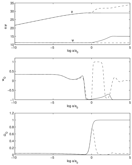
Figure 1: Evolution of the quintessence fields (upper panel), the equation of state parameter (middle panel) and the quintessence fractional energy density (lower panel), for transient (dashed) and permanent (full) acceleration solutions.

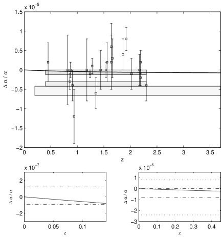
Figure 2: Evolution of $\alpha$ for a transient acceleration model with $\zeta_{1}=2\times 10^{-6}$ and $\zeta_{2}=8\times 10^{-5}$. In the upper panel, the boxes represent the QSO bounds given in Eqs. (2) (top box), (3) (middle box) and (1) (lower box). Also shown is the QSO absorption systems dataset of Chand et al. (Table 3 of Ref. Chand1 ). The lower panel details the behaviour of $\alpha$ for small values of $z$. The lower left plot shows the Oklo bound (dash-dotted lines) and the right one the meteorite bounds (dash-dotted and dotted lines correspond to $1\sigma$ and $2\sigma$, respectively).

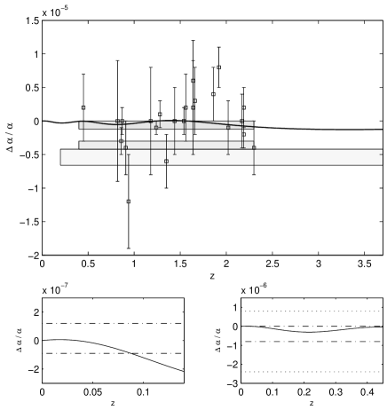
Figure 3: As for Fig. 2 but for a permanent acceleration model with $\zeta_{1}=-4\times 10^{-5}$ and $\zeta_{2}=1\times 10^{-6}$.

Integrating Eqs. (17), one finds that there are essentially two realistic types of solutions, corresponding to either transient or permanent acceleration, as illustrated in Figure 1. It is possible to obtain permanent or transient vacuum domination, satisfying present bounds on observable cosmological parameters, for a rather broad range of parameters of the potential, as discussed in Bento:2001yv .

Permanent vacuum domination takes place when at least the $\phi$ field settles at the minimum of the potential; soon after, $\psi$ monotonically increases until it reaches its asymptotic value. For transient vacuum domination (which occurs either when the potential has no local minimum or when $\phi$ arrives at the minimum with enough kinetic energy to roll over the potential barrier) the $\phi$ field increases monotonically and $\psi$ slightly decreases. The contribution of $P(\phi,\psi)$, which controls the presence and location of the minimum, is only important at recent times, since at early epochs the exponential factor dominates and the model behavior depends essentially on parameter $\lambda$. Notice that, as $\lambda$ increases, the model becomes more similar to $\Lambda$CDM at early times.

The interaction term between the scalar fields and the electromagnetic field is, as suggested in Ref. Bekenstein ,

$${\cal L}_{em}=-\frac{1}{4}B_{F}(\phi,\psi)F_{\mu\nu}F^{\mu\nu}~{},$$ (19)

with a linearly expanded $B(\phi,\psi)$ given by

$$B_{F}(\phi,\psi)=1-\zeta_{1}(\phi-\phi_{0})-\zeta_{2}(\psi-\psi_{0}),$$ (20)

where $\phi_{0}$ and $\psi_{0}$ are the present values of the scalar fields. Therefore, the variation of the fine structure constant, $\alpha=\alpha_{0}/B_{F}(\phi,\psi)$, is given by

$${\Delta\alpha\over\alpha}=\zeta_{1}(\phi-\phi_{0})+\zeta_{2}(\psi-\psi_{0})\,.$$ (21)

Notice that the upper bound on $\zeta_{F}$, see Eq. (12), implies that $\zeta_{1,2}\leq 7\times 10^{-4}$ because of the different definition for $B_{F}$ used in Olive:2001vz , namely, $B_{F}(\varphi)=1-{\zeta_{F}\over M_{*}}(\varphi-\varphi_{0})$.

The rate of variation of $\alpha$, at present, can be written as

$${\dot{\alpha}\over\alpha}=-\left(\zeta_{1}{d\phi\over dy}~{}+\zeta_{2}{d\psi\over dy}\right)H_{0}\,,$$ (22)

where $y\equiv 1+z$ and $H_{0}$ is the value of the Hubble constant at present, $H_{0}=(h/9.78)~{}\times 10^{-9}~{}{\rm yr}^{-1}$.

III Results

We adopt the method of choosing the model parameters so as to satisfy a set of priors for the cosmological parameters ($h=0.70$, $\Omega_{m}=0.3$, $\Omega_{Q}=0.70$ and $\Omega_{r}=4.15\times 10^{-5}h^{-2}$) and then adjust the coupling parameters, $\zeta_{1}$ and $\zeta_{2}$, in order to satisfy the bounds on the evolution of $\alpha$. Notice that the priors chosen above are consistent with a combination of WMAP data and other CMB experiments (ACBAR and CBI), 2dFGRS measurements and Lyman $\alpha$ forest data, which gives Spergel:2003cb : $h=0.71^{+0.04}_{-0.03}$, $\Omega_{m}=0.27\pm 0.04$, $\Omega_{Q}=0.73\pm 0.04$ and $w_{Q}<-0.78$ ($95\%$ CL), corresponding to the best fit for the observed Universe.

For large $z$, the tightest bound on dark energy arises from nucleosynthesis, $\Omega_{Q}(z=10^{10})<0.045$, implying that $\lambda>9$ Bean . Considering a possible underestimation of systematic errors, one gets a more conservative bound, $\Omega_{Q}<0.09$ at $2\sigma$, which corresponds to $\lambda>6.5$. For the model parameters chosen in this work (see below), we get $\Omega_{Q}=0.042$.

The model is also consistent with CMBR observations. Recent CMBR data imply that $\Omega_{Q}<0.39$ at last scattering Bean , which is less stringent than the nucleosynthesis bound and is clearly obeyed by our model. We have also computed the angle subtended by the sound horizon at last scattering, obtaining $\theta_{A}\simeq 0.599^{o}$, clearly within WMAP bounds on this quantity Spergel:2003cb : $\theta_{A}=0.598\pm 0.002^{o}$.

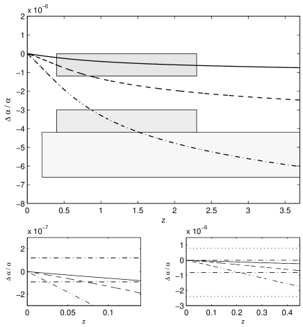
Figure 4: Evolution of $\alpha$ for a transient acceleration model with $\zeta_{1}=2\times 10^{-6}$ and $\zeta_{2}=8\times 10^{-5}$ (full line), $\zeta_{1}=5.3\times 10^{-6}$ and $\zeta_{2}=3\times 10^{-5}$ (dashed line), $\zeta_{1}=1.4\times 10^{-5}$ and $\zeta_{2}=7\times 10^{-4}$ (dash-dotted line). Line and box conventions are those of Figs. 2 and 3.

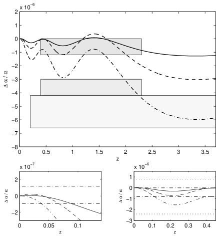
Figure 5: As for Fig. 4 but for a permanent acceleration model with $\zeta_{1}=-4\times 10^{-5}$ and $\zeta_{2}=1\times 10^{-6}$ (full line), $\zeta_{1}=-1\times 10^{-4}$ and $\zeta_{2}=1\times 10^{-6}$ (dashed line), $\zeta_{1}=-1.5\times 10^{-4}$ and $\zeta_{2}=1.4\times 10^{-5}$ (dash-dotted line).

As an example of transient acceleration models, we consider the following set of parameters: $\lambda=9.5$, $A=0.1$, $B=10^{-3}$, $C=8\times 10^{-5}$, $D=2.8$, $\phi_{*}=28.965$, $\psi_{*}=20$, with $\zeta_{1}=2\times 10^{-6}$ and $\zeta_{2}=8\times 10^{-5}$. In this case, the variation of $\alpha$ is in agreement with both the Oklo and meteorite bounds, as can be seen in the lower panel of Figure 2. In the upper panel, we see that the fit to Chand et al. QSO data (where terrestrial isotopic abundances have been assumed) is acceptable: we get $\chi^{2}/d.o.f=22/15$ (notice that, in the computation of the $d.o.f.$, only 8 free variables should be taken into account since one potential parameter is tuned in order to have the observed dark energy density at the present). Also the constraint from atomic clock measurements is verified as we obtain

$${{\dot{\alpha}\over\alpha}}=-4.5\times 10^{-17}~{}\mbox{yr}^{-1}~{}.$$ (23)

Moreover, the model gives variations in $\alpha$ during BBN and at the last scattering surface well within the bounds stated earlier, e.g. we get

$${\Delta\alpha\over\alpha}(CMBR)=-2.7\times 10^{-6}~{},$$

$${\Delta\alpha\over\alpha}(BBN)=-1.1\times 10^{-6}~{}.$$ (24)

For models with permanent acceleration, however, consistency with QSO spectra and Oklo data is problematic. Our results are illustrated in Figure 3, where we have chosen $\lambda=9.5$, $A=0.02$, $B=2\times 10^{-3}$, $C=6\times 10^{-4}$, $D=4.5$, $\phi_{*}=28.9675$, $\psi_{*}=15$, for $\zeta_{1}=-4\times 10^{-5}$ and $\zeta_{2}=1\times 10^{-6}$. We get

$${{\dot{\alpha}\over\alpha}}=5.2\times 10^{-17}~{}\mbox{yr}^{-1}$$

$${\Delta\alpha\over\alpha}(CMBR)=4.5\times 10^{-5}$$

$${\Delta\alpha\over\alpha}(BBN)=2.9\times 10^{-4}$$ (25)

and $\chi^{2}/d.o.f=21/15$. Notice that the BBN bound is not respected in this case.

It is clear that the evolution of $\alpha$, past and future, is a reflection of the dynamics of the fields $\phi$ and $\psi$, which depends crucially on whether acceleration is permanent or transient. In the example of Figure 2, $\alpha$ is increasing monotonically and will continue to do so. However if $\zeta_{1}\ll\zeta_{2}$, it is the $\psi$ field that determines the evolution; hence, in that case, $\alpha$ may decrease in the future. For permanent acceleration solutions, the sign of $\zeta_{2}$ determines the future evolution of $\alpha$, since $\psi$ has more dynamics than $\phi$. Hence, for the example of Figure 3, $\alpha$ will increase in the future since $\zeta_{2}>0$; the oscillating behavior of $\alpha$ reflects the oscillations of $\phi$ before it settles at the minimum of the potential.

In Figs. 4 and 5 we show that, increasing the couplings to the electromagnetic field, $\zeta_{1}$ and $\zeta_{2}$, it is also possible to fit Murphy et al. QSO data Murphy:2003hw , both in the transient and permanent acceleration regimes. However, as should be expected, it is more difficult to respect the Oklo and meteorites bounds in both cases.

IV Conclusions

In this work, we have studied the variation of the fine structure constant in the context of a quintessence model with two coupled scalar fields. We find that transient acceleration models can fit the latest QSO data and comply with the upper bounds on $\Delta\alpha$ from the Oklo reactor, meteorite analysis and the atomic clock measurements. For permanent acceleration models, however, it is more difficult to fit the QSO data and satisfy the Oklo, meteorite and BBN bounds simultaneously. We have studied the sensitivity of our results to $\zeta_{1}$ and $\zeta_{2}$, the couplings of quintessence fields with electromagnetism, and we have found that, in order to be consistent with the data, these parameters must be at least one order of magnitude smaller than the upper bound implied by the Equivalence Principle.

On a more general ground, we could say that establishing whether there is a variation of the fine structure constant and, in the affirmative case, identifying its origin, remains a difficult task before a deeper analysis of the systematic errors of the observations and studies of the degeneracies with the various cosmological parameters. This is particularly evident in what concerns the compatibility of the datasets of Murphy et al. and Chand et al.

- (1) M.T. Murphy, J.K. Webb and V.V. Flambaum, Mon. Not. Roy. Astron. Soc. 345, 609 (2003).
- (2) M.T. Murphy, J.K. Webb, V.V. Flambaum and S.J. Curran, Astrophys. Space Sci. 283, 577 (2003); J.K. Webb et al., Phys. Rev. Lett. 87, 091301 (2001); M.T. Murphy et al., Mon. Not. Roy. Astron. Soc. 327, 1208 (2001).
- (3) M.T. Murphy, J.K. Webb, V.V. Flambaum, J.X. Prochaska and A.M. Wolfe, Mon. Not. Roy. Astron. Soc. 327, 1237 (2001).
- (4) M.T. Murphy, J.K. Webb, V.V. Flambaum, M.J. Drinkwater, F. Combes and T. Wiklind, Mon. Not. Roy. Astron. Soc. 327, 1244 (2001).
- (5) J.D. Bekenstein, Phys. Rev. D 25, 1527 (1982).
- (6) K.A. Olive and M. Pospelov, Phys. Rev. D 65, 085044 (2002).
- (7) C.L. Gardner, Phys. Rev. D 68, 043513 (2003).
- (8) L. Anchordoqui and H. Goldberg, Phys. Rev. D 68, 083513 (2003); E.J. Copeland, N.J. Nunes, and M. Pospelov, Phys. Rev. D 69, 023501 (2004); J. Khoury and A. Weltman, astro-ph/0309411; D-S Lee, W. Lee and K-W Ng, astro-ph/0309316.
- (9) D.F. Mota and J.D. Barrow, astro-ph/0309273.
- (10) V.A. Kostelecký, R. Lehnert and M.J. Perry, Phys. Rev. D 68 123511 (2003).
- (11) O.Bertolami, R. Lehnert, R. Potting and A. Ribeiro, Phys. Rev. D, in press, astro-ph/0310344.
- (12) M.C. Bento, O. Bertolami and N.M.C. Santos, Phys. Rev. D 65, 067301 (2002).
- (13) A.A. Linde, Phys. Lett. B249 18 (1990); M.C. Bento, O. Bertolami and P.M. Sá, Phys. Lett. B262 11 (1991); Mod. Phys. Lett. A7 (1992) 911; L. Kofman, A. Linde and A.A. Starobinsky, Phys. Rev. Lett. 76 1011 (1996); Phys. Rev. D56 3258 (1997); O. Bertolami and G.G. Ross, Phys. Lett. B171 163 (1986).
- (14) S. Hellerman, N. Kaloper and L. Susskind, JHEP 0106, 003 (2001) W. Fischler, A. Kashani-Poor, R. McNess and S. Paban, JHEP 0107, 003 (2001); E. Witten, hep-th/0106109.
- (15) H. Chand, R. Srianand, P. Petitjean and B. Aracil, astro-ph/0401094;
- (16) R. Srianand, H. Chand, P. Petitjean and B. Aracil, astro-ph/0402177.
- (17) T. Damour and F. Dyson, Nucl. Phys. B 480, 37 (1996).
- (18) Y. Fujii, Phys. Lett. B 573, 39 (2003).
- (19) Y. Fujii et al., Nucl. Phys. B 573, 377 (2000).
- (20) S. K. Lamoreaux, nucl-th/0309048.
- (21) K.A. Olive, M. Pospelov, Y.Z. Qian, G. Manhes, E. Vangioni-Flam, A. Coc and M. Casse, Phys. Rev. D 69, 027701 (2004).
- (22) Y. Fujii and A. Iwamoto, Phys. Rev. Lett. 91, 261101 (2003).
- (23) K.A. Olive, M. Pospelov, Y.Z. Qian, A. Coc, M. Casse and E. Vangioni-Flam, Phys. Rev. D 66, 045022 (2002).
- (24) H. Marion et al., Phys. Rev. Lett. 90, 150801 (2003).
- (25) S. Bize et al., Phys. Rev. Lett. 90 150802 (2003).
- (26) M. Fischer et al., physics/0312086.
- (27) R.A. Battye, R. Crittenden and J. Weller, Phys. Rev. D 63, 043505 (2001); C.J.A. Martins, A. Melchiorri, G. Rocha, R. Trotta, P.P. Avelino and P. Viana, astro-ph/0302295.
- (28) S. Hannestad, Phys. Rev. D 60, 023515 (1999); M. Kaplinghat, R.J. Scherrer and M.S. Turner, Phys. Rev. D 60, 023516 (1999); S.J. Landau, D.D. Harari and M. Zaldarriaga, Phys. Rev. D 63, 083505 (2001).
- (29) L. Bergstrom, S. Iguri and H. Rubinstein, Phys. Rev. D 60, 045005 (1999); K. Ichikawa and M. Kawasaki, Phys. Rev. D 65, 123511 (2002); K.M. Nollett and R.E. Lopez, Phys. Rev. D 66, 063507 (2002).
- (30) R. Bean, S.H. Hansen and A. Melchiorri, Phys. Rev. D 64, 103508 (2001).
- (31) A. Albrecht and C. Skordis, Phys. Rev. D 84 2076 (2000).
- (32) D.N. Spergel et al., Astrophys. J. Suppl. 148, 175 (2003). C. L. Bennett et al., Astrophys. J. Suppl. 148, 1 (2003).