THE X-RAY DERIVED COSMOLOGICAL STAR FORMATION HISTORY AND THE GALAXY X-RAY LUMINOSITY FUNCTIONS IN THE Chandra DEEP FIELDS NORTH AND SOUTH

Abstract

The cosmological star formation rate in the combined Chandra Deep Fields North and South is derived from our X-Ray Luminosity Function for Galaxies in these Deep Fields. Mild evolution is seen up to redshift order unity with SFR $\sim(1+z)^{2.7}$. This is the first directly observed normal star-forming galaxy X-ray luminosity function (XLF) at cosmologically interesting redshifts (z$>$0). This provides the most direct measure yet of the X-ray derived cosmic star-formation history of the Universe.

We make use of Bayesian statistical methods to classify the galaxies and the two types of AGN, finding the most useful discriminators to be the X-ray luminosity, X-ray hardness ratio, and X-ray to optical flux ratio. There is some residual AGN contamination in the sample at the bright end of the luminosity function. Incompleteness slightly flattens the XLF at the faint end of the luminosity function.

The XLF has a lognormal distribution and agrees well with the radio and infrared luminosity functions. However, the XLF does not agree with the Schechter luminosity function for the H$\alpha$LF indicating that, as discussed in the text, additional and different physical processes may be involved in the establishment of the lognormal form of the XLF.

The agreement of our star formation history points with the other star formation determinations in different wavebands (IR, Radio, H$\alpha$) gives an interesting constraint on the IMF. The X-ray emission in the Chandra band is most likely due to binary stars although X-ray emission from non-stellar sources (e.g., intermediate-mass black holes and/or low-luminosity AGN) remain a possibility. Under the assumption it is binary stars the overall consistency and correlations between single star effects and binary star effects indicate that not only is the one parameter IMF(M) constant but also the bivariate IMF($M_{1},M_{2}$) must be constant at least at the high mass end. Another way to put this, quite simply, is that X-ray observations may be measuring directly the binary star formation history of the Universe.

X-ray studies will continue to be useful for probing the star formation history of the universe by avoiding problems of obscuration. Star formation may therefore be measured in more detail by deep surveys with future x-ray missions.

1. Introduction

There have been many recent studies of star formation in galaxies and of the star formation history of the universe derived from data in the radio, IR, and optical (Lilly et al., 1996; Madau et al., 1998; Rowan-Robinson et al., 1997; Haarsma et al., 2000; Cole et al., 2001; Baldry et al., 2002; Teplitz et al., 2003). In the range from the present epoch to redshifts of order unity, recent critical compilations and discussions of Sullivan et al. (2001), Hopkins et al. (2003), Sullivan et al. (2004) and Hogg (2004) show that the results from the multi-waveband data have a dispersion of 1-2 orders of magnitude in the comoving cosmic star formation density . As noted by these authors, there are important physical corrections that need to be made to go from the observations in a particular band to the cosmic star formation rate which include physical understanding of the dust extinction, the Initial Mass function (IMF), and stellar population models. Reasonable interpretations of the current observations in this redshift range have been presented that argue, on the one hand, that there is a steep decline in the star formation rate to the present epoch Hogg (2004) or, on the other, that the cosmic star formation density has a shallow decline in the same redshift range Wilson, Cowie, Barger & Burke (2002). Therefore it is important to utilize all wavebands to study this phenomenon from different aspects and with different selection effects. The X-ray band has now just opened up to detailed studies of star formation in galaxies at cosmological distances.

Hitherto, even deep X-ray surveys studied only the cosmological populations of evolving active galaxies and quasars. X-ray studies of individual nearby galaxies were performed and the underlying hot gas and stellar x-ray source components analyzed (Fabbiano, 1989). However, the deep 1-2 Megasecond surveys in the Chandra Deep Field South and North, respectively, now show a major cosmological population (in the range from present day to redshifts of order unity) of X-ray emitting normal star forming galaxies at faint flux levels. Stacking analysis allows one to extend the x-ray properties studied to even larger redshift ranges (Hornschemeier et al., 2002).

Some notable results on star-forming galaxies have already been derived in deep X-ray survey work. In the $Chandra$ Deep Field-North (hereafter CDF-N) it has been found that the faint 15$\mu$m population, composed primarily of luminous infrared starburst galaxies (e.g. Chary & Elbaz (2001)) are associated with X-ray-detected emission-line galaxies (Alexander et al. 2002). Chandra and XMM-Newton stacking analyses of relatively quiescent (non-starburst) galaxies have constrained the evolution of X-ray emission with respect to optical emission to at most a factor of 2–3 (e.g., Hornschemeier et al. 2002; Georgakakis et al. 2003). Studies of the quiescent population of galaxies has also provided some initial constraints on the evolution of star-formation in the Universe ( SFR $\sim(1+z)^{k}$ for $z<<1$ where k $<3$; Georgakakis et al. 2003).

We now discuss some relevant details of the X-ray observations. We derive X-ray Luminosity Functions and the corresponding cosmological star formation history using X-ray data from the 2 Ms and 1 Ms exposures of the CDF-N and Chandra Deep Field South (hereafter CDF-S). This analysis requires the extreme depth of the CDF surveys as non-active galaxies arise in appreciable numbers at extremely faint X-ray fluxes; the fraction of X-ray sources that are normal and star-forming galaxies rises sharply below 0.5–2 keV fluxes of $\approx 1\times 10^{-15}$ erg cm^-2 s^-1 (e.g., Figure 6 of Hornschemeier et al., 2003, ; see also the fluctuation analysis results of Miyaji & Griffiths 2002).

The luminosity functions for galaxies in the radio, optical and infrared have been studied extensively (c.f. Tresse et al. (2002) for a recent discussion). Prior to this work, the X-ray luminosity function for normal galaxies was estimated from the optical galaxy luminosity function by Georgantopoulus, Basilakos & Plionis (1999). Schmidt, Boller & Voges (1996) reported on a galaxy XLF derived in the local ($v<500$ km s^-1) Universe as well, however their sample does include some fairly active galaxies (e.g., Cen A) and does not appear to be an entirely clean normal/star-forming galaxy luminosity function. Our work seeks to construct a relatively clean normal star-forming galaxy luminosity function, and possesses the great advantage of doing this at cosmologically interesting distances (our two luminosity functions have median redshifts $z\approx 0.3$ and $z\approx 0.8$). We may thus study the evolution of X-ray emission from galaxies with respect to cosmologically varying quantities such as the global star-formation density of the Universe. Our galaxy XLFs have their own set of selection effects that we discuss later but they can add to the overall picture of the physics of galaxy evolution. For example, it is obvious that corrections for obscuration will not be as important here as in the analysis of H$\alpha$ Luminosity functions discussed in detail below.

We expect correlations between the various classic cosmological indicators of star formation (H$\alpha$, IR, radio) and our X-ray studies. In general, the fluxes we measure in the respective wavebands associated with the different methods are all ultimately connected with the evolution and death and transfiguration of massive stars. For example, the radiative luminosity of OB stars, the mechanical energy input from supernovae and the accretion power of high mass X-ray binaries (HMXBs) are all ultimately derived from massive stars. It is therefore not surprising that tight correlations have been found empirically between the X-ray flux, the radio flux and the IR continuum. The most recent careful analysis in the local Universe is from Ranalli, Comastri & Setti (2003) which is discussed in detail below. Interestingly, the correlations appear to hold for at least the radio and X-ray bands at high redshift Bauer et al. (2002); Grimm, Gilfanov & Sunyaev (2003). We use these latest empirically derived correlations betwen radio, IR, and X-ray star formation indicators as the central relations that allow us to infer star formation rates from the X-ray data on galaxies in the Chandra Deep Fields North and South. In addition, it is useful to also consider theoretical studies on the cosmic X-ray evolution of galaxies which have been presented by Cavaliere, Giacconi & Menci (2000), Ptak et al. (2001) and Ghosh & White (2001).

Observations of detailed X-ray stellar populations in individual nearby galaxies have been carried out by Zezas & Fabbiano (2002),Kilgard et al. (2002) and Colbert et al. (2003). Using archival $Chandra$ data on 32 galaxies in the nearby Universe, Colbert et al. (2003) have established that the X-ray emission from accreting binaries in galaxies is correlated with the current level of star formation in their host galaxies. This relation appears to be both macroscopic in that the entire X-ray point source luminosity of galaxies scales with star-formation rate and microscopic in that the slope of the X-ray binary luminosity function within galaxies correlates with star formation.

In our studies, much care has gone into accurately selecting the population of normal star forming galaxies. Contamination by AGNs is a potentially serious problem. We have a multi-parameter probability space for the selection of the normal star forming galaxies and we have therefore used Bayesian methods to classify the galaxies and the two types of AGN. The most useful discriminators are the X-ray luminosity and X-ray hardness ratio as well as the optical to X-ray ratios. AGN contamination is most serious at the bright end of the luminosity function. Our analysis is a step towards a fully modern statistical Monte Carlo Markov-Chain study but we need to have a better idea of the overall structure of the probability space before we undertake this (c.f. Hobson, Bridle and Lahav (2002) and Hobson & McLachlan (2003)). Our analysis assumes, as a first step, that the priors are Gaussian and we show that this is a reasonable and useful assumption.

These studies of the cosmological evolution of normal star forming galaxies in the x-ray bands are the first of many detailed studies that can be undertaken with future missions such as XEUS. Here we have made a start on the basic luminosity functions and cosmic star formation histories.

The organization of this Paper is as follows: in section 2 we describe the data acquisition, the selection of the galaxy sample and the processing of the data. Section 3 presents the derivation of the galaxy XLF. In Section 4, we carefully compare the galaxy XLF derived here with the IR LF using the recent empirically derived analysis from Ranalli, Comastri & Setti (2003) (hereafter RCS). A similar procedure is undertaken for comparison with the H$\alpha$LF. We also give the derived cosmic star formation rates from the XLF. In section 5 we discuss the implications of our results and the potential consequences for future missions. In section 6 we give our four principal conclusions. Throughout this paper, if not explicitly stated otherwise, we use $H_{0}$ = 70 km s^-1 Mpc^-1, $\Omega_{m}=0.3$ and $\Omega_{\Lambda}=0.7$.

2. Data Acquisition, Selection of Galaxies, and Data Reduction

2.1. Data Acquisition

2.1.1 CDF-S

From October 1999 to Dec 2000, 11 individual exposures of the CDF-S were performed with the Chandra ACIS instrument, resulting in a 1 Ms exposure. The sensitivity of this deep exposure has reached flux limits of $5.5\times 10^{-17}$ erg cm^-2 s^-1 in the soft band (0.5–2 keV) and $4.5\times 10^{-16}$ erg cm^-2 s^-1 in the hard band (2–10 keV). At these flux levels, $>$ 80$\%$ of the cosmic X-ray background in both bands is resolved. A total of 346 sources has been detected (Rosati et al., 2002; Giacconi et al., 2002); the X-ray data reduction, source detection, and X-ray source catalog can be found in Giacconi et al. (2002). The optical spectroscopic follow-up observations were obtained using FORS1/FORS2 on the VLT for the possible optical counterparts of 238 X-ray sources, yielding spectroscopic redshifts for 141 X-ray sources. The optical spectra and the redshifts are presented in Szokoly et al. (2004). Zheng et al., in preparation, have used the ten near-UV, optical, and near-infrared bands to estimate photometric redshifts for 342 (99%) of the CDF-S sources, making detailed comparison with the spectroscopic redshifts. In some cases, the optical spectroscopic redshifts of Szokoly et al. were not highly confident and Zheng et al. was able to place a better redshift constraint using the multiwavelength SED of the sources. We therefore used those redshifts of Zheng et al. which we consider to supercede those of Szokoly et al.

2.1.2 CDF-N

From November 1999 to February 2002, 20 individual exposures of the CDF-N were performed by the Chandra ACIS instrument, resulting in a 2 Ms exposure. In the central parts of the CDF-N the sensitivity reaches $2.5\times 10^{-17}$ erg cm^-2 s^-1 in the 0.5–2 keV band and $1.4\times 10^{-16}$ erg cm^-2 s^-1 in the 2–8 keV band. the 1 Ms survey; 503 sources were detected in the 2 Ms data, and the X-ray data reduction, source detection, and X-ray source catalog can be found in Alexander et al. (2003). The optical spectroscopic and photometric follow-up observations were obtained using Keck and Subaru (Barger et al., 2002, 2003). Spectroscopic redshifts have been obtained for 284 of CDF-N X-ray sources; using the multiwavelength photometric data, photometric redshifts were obtained for an additional 78 sources Barger et al. (2003). We use these 362 redshifts in our study. Note that although the overall completeness is roughly 71%, including the photometric redshifts, the spectroscopic completeness alone for R $\leq 24$ is 87%. The optical and near-infrared photometry, spectroscopic redshifts, and photometric redshifts are presented in Barger et al. (2003).

2.2. Galaxy Selection

In our study it is essential to classify galaxies correctly. We have employed two different galaxy classification techniques. The first method uses standard optical classification for sources with high-quality optical spectra. The second approach utilizes a multi-parameter Bayesian analysis.

We have chosen to construct XLFs in the 0.5–2 keV band since for moderately obscured AGN with significant star formation present, the soft band is dominated by star forming processes (Ptak et al., 1999; Levenson, Weaver, & Heckman, 2001; Terashima et al., 2002).

2.2.1 Optical Spectroscopic Classification

Very few galaxies have optical spectra with good enough signal-to-noise to allow classifications based on emission-line flux ratios. Therefore, it is essential that we develop a classification scheme which is not dependent (or overly dependent) upon optical spectroscopic classification. However, there is important optical spectroscopic information contained within the spectra. For the CDF-S spectra with sufficient signal-to-noise, we have used the diagnostic diagrams of Rola, Terlevich & Terlevich (1997) in a manner similiar to Kewley et al. (2002). Where only one or two emission lines are present, we classify the objects as AGN if broad features or high ionization lines were present and galaxies otherwise. Note that the classifications in most of the optical spectroscopic follow-up work in the Chandra Deep Fields, e.g., Szokoly et al. (2004), are based upon both X-ray (luminosities and hardness ratios) and optical properties. We do not consider the X-ray properties in classifying these galaxies as we are using them to construct our X-ray prior.

There are 29 galaxies whose emission-line ratios are consistent with starbursts and/or normal galaxies rather than AGN. We further exluded two of these sources since they were found at off-axis angle in excess of 8’ where the spectroscopic completeness considerably worsens relative to the center of the survey (Szokoly et al. 2004). This is thus our “spectroscopic CDF-S sample” with a total of 27 galaxies. Note that we do not classify an analogous “spectroscopic CDF-N sample” as those optical spectra are not available, and also are generally not flux calibrated (Barger et al., 2003), which would prevent line ratios from being calculated.

2.2.2 Multi-parameter Classification: $(f_{x}/f_{R})$, HR, $L_{X}$

Even with optical classification there is still the risk of AGN contamination, particularly for type-2 AGN where the AGN may be obscured and/or the spectral aperture encompasses the entire galaxy (e.g., Moran, Filippenko & Chornok, 2002). Therefore, we used a second selection approach based on the statistical properties of the sources.

For this statistical analysis we concentrated on the CDF-S multiwavelength data since again we had access to the optical spectra of potential counterparts, and could therefore most reliably identify control sets of galaxies and AGN. We investigated the distributions of the X-ray hardness ratios and 1.4 GHz, K-band, R-band and soft X-ray luminosities and inferred that a good discriminator between AGN and galaxies was based on the X-ray/optical luminosity ratio, the X-ray hardness ratio and X-ray luminosity as had been found previously (Hasinger, 2003, and references therein). The ratios $L_{X}/L_{1.4\ \rm GH}$ and $L_{X}/L_{\rm K}$ also show promise and will be explored in future work.

In Figure 1 we plot the hardness ratio vs soft band X-ray luminosity of all CDF-S sources with good spectroscopic redshifts and classifications. Different symbols are used for the various optical spectroscopic classifications (type 1 AGN, hereafter AGN1; type 2 AGN; hereafter AGN2 and normal galaxies). It is evident that the AGN1 and galaxies have similar hardness ratios and AGN1 have significantly higher X-ray luminosities. AGN2 span a larger range in X-ray luminosity than AGN1 and on average have harder spectra than AGN1 and galaxies. Both of these effects are expected since AGN2 are generally X-ray-obscured sources. A brief synopsis of the technique follows.

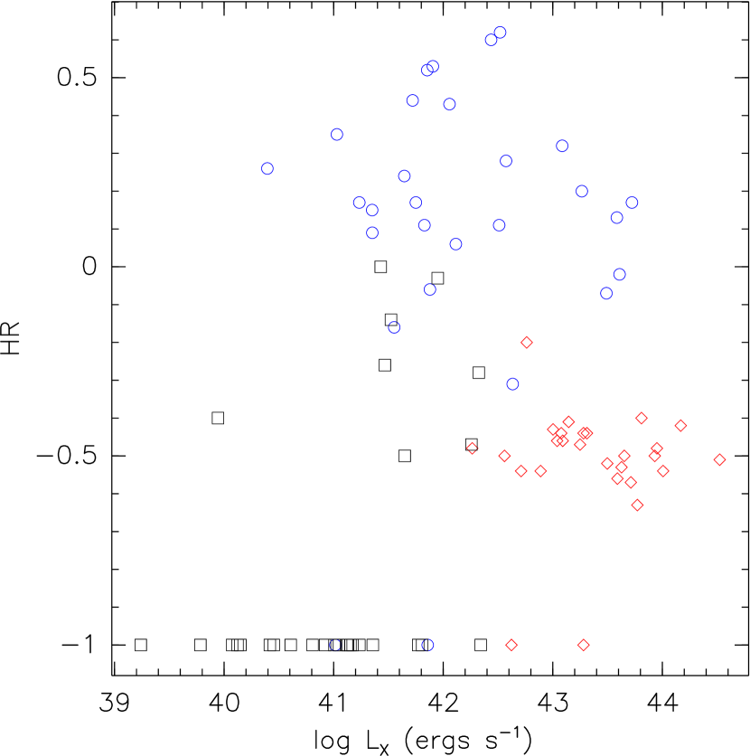
Figure 1.— X-ray hardness ratio HR vs. soft X-ray (0.5 – 2.0 keV) luminosities for CDF-S sources with spectroscopic redshifts and classification. Galaxies are plotted as black squares, AGN1 are red diamonds and AGN2 are blue circles. All luminosities are calculated assuming $H_{0}$ = 70 km s^-1 Mpc^-1, $\Omega_{m}=0.3$ and $\Omega_{\Lambda}=0.7$ .

In most cases the errors on the hardness ratios are large for sources in the galaxy regime as there were often only a few X-ray counts (i.e., $\log{L_{X}}<42$ and HR $<0$) and, in fact, many sources in this regime only have upper-limits for HR. Our selection approach takes into account the errors on the hardness ratios and the parent distribution properties discussed above. This approach is described in Appendix A, and we also restricted our sample to sources with redshifts $\leq 1.2$ (since the redshift estimates for the sources become increasingly uncertain at higher redshifts and our two redshift bins should be of comparable size). This resulted in 74 CDF-S and 136 CDF-N sources being classified as galaxies. In Figure 2 we show the redshift distribution for the (Bayesian) galaxy sample.

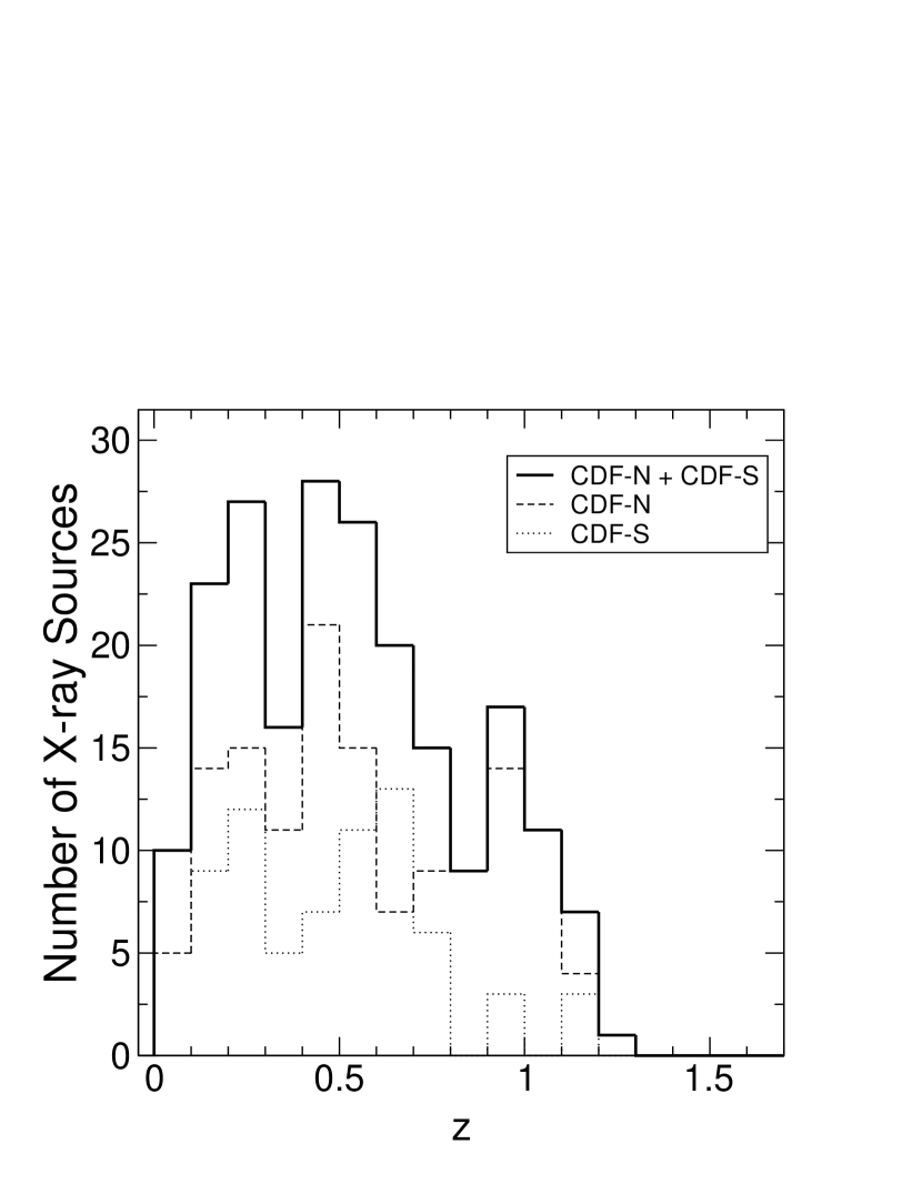
Figure 2.— The redshift distribution of the Bayes-selected galaxy sample.

3. Luminosity Functions

The standard method of constructing binned luminosity functions discussed in Page & Carrera (2000) was used in this paper to calculate the soft X-ray luminosity function for normal galaxies (see also Schmidt, 1968; Miyaji, Hasinger & Schmidt, 2000, 2001) . For each redshift and X-ray luminosity bin, the source density, $\phi$, can be estimated from $\phi\sim N(\int_{L_{min}}^{L_{max}}\int_{z_{min}}^{z_{max}(L)}(dV_{c}/dz)dzdL)^{-1}$, where N is the number of sources in the bin, $L_{min}$ and $L_{max}$ are the minimum and maximum X-ray luminosities of each bin, and $dV_{c}/dz$ is the total comoving volume per redshift interval, dz, that the CDF surveys can reach at each luminosity L. For a given luminosity L_X, $z_{min}(L)$ is the minimum redshift of the bin and $z_{max}(L)$ is the highest redshift possible for a source of luminosity L for it to remain in the redshift bin. The variance of the source densities can also be estimated from $\delta\phi\sim\delta N(\int_{L_{min}}^{L_{max}}\int_{z_{min}}^{z_{max}(L)}(dV/dz)dzdL)^{-1}$where $\delta$N is the $1\sigma$ Poisson error for the number of sources in each bin (Kraft, Burrows, & Nousek, 1991; Gehrels, 1986). The XLF derived from the Bayesian sample is shown in Figure 3 and the spectroscopic CDF-S sample XLF is shown in Figure 4.

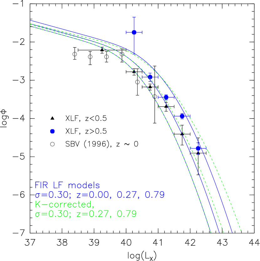
Figure 3.— Combined CDF-N and CDF-S XLF based on the Bayesian model testing sample (see text for details) along with the 60$\mu$m LF from Takeuchi, Yashikawa, & Ishii (2003) converted to the 0.5-2.0 keV bandpass using the $L_{60\mu m}$/X-ray correlation (based on the galaxy sample given in Ranalli et al. [2003]). The left panel shows the 60$\mu$m LF model based on the full IRAS PSCz sample while right panels shows the LF based on the “warm” galaxy sample (with $S_{100\mu m}/F_{60\mu m}<2.1$). The X-ray data in both plots are identical, and evidently the warm galaxy LF more closely matches the XLF at each redshift. The XLF was computed with redshifts z $<$ 0.5 and z $>$ 0.5. Also plotted (as open circles) is the local XLF derived in Schmidt, Boller, & Voges (1996), corrected for the factor of $\sim 3$ overdensity of galaxies locally (see text). Curves are plotted for z=0 and the mean redshifts of the two XLF samples ($z=0.27$,$z=0.79$), with the z$>$0 curves being calculated assuming (1+z)^2.7 evolution. The dashed curves show the (minor) effect of including an estimate of X-ray k-corrections when converting from FIR to X-ray 0.5-2.0 keV luminosities. The y axis units are log (Mpc${}^{-}3$ dex^-1).

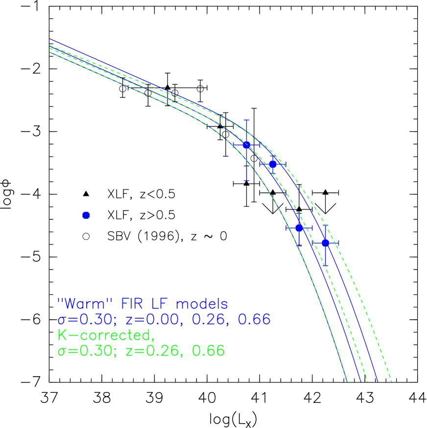
Figure 4.— The CDF-S spectroscopic galaxy sample (see text for details). Curves and symbols are as in Figure 3, with the 60 $\mu m$ “warm” galaxy LF model being used here. The XLF shown here were corrected for completeness, which only impacted the first bin of each XLF signficantly (see text).

In the case of the spectroscopic CDF-S sample we also made an approximate correction for spectroscopic completeness. We used the mean $\log F_{X}/F_{opt}$ value for galaxies (-1.7 as discussed in the Appedix) to compute the range in R magnitude corresponding to each XLF bin, and took the fraction of redshifts in that interval (using all sources in Szokoly et al. (2004), restricted to a maximum off-axis angle of 8’) as an estimate of the completeness. Often in the higher luminosity bins there were not a large enough number of sources for the fraction to be computed accurately however we found that the completeness when R$<$ 23 was consistently $\sim 90\%$, and therefore we fixed the completeness at 90% whenever the entire higher R range for that bin was $<$ 23. This procedure only significantly impacted the first point of each XLF, with completenesses of 43% and 73% for the z$<$0.5 and z$>$0.5 XLFs, respectively.

3.1. X-ray Luminosity Function Evolution

3.1.1 Form of the X-ray Luminosity Function

To describe the evolution of the X-ray luminosity in more detail it is useful to use a functional form for the XLFs we have obtained above. It is then easy to test simple models for evolution of the XLFs such as pure luminosity evolution (PLE). The choice of the appropriate functional fit should, if possible, have a solid basis in physical understanding and in empirical observational correlation. After trying various forms we chose to use the lognormal distribution. The infrared luminosity function of galaxies (IRLF) is well fit by this distribution. In addition, the IRLF is known to be directly proportional to the star-formation rate (Kennicutt, 1998). We established that this form of the distribution is a reasonable fit to our XLF data. Then, to give the XLF a more physical basis, we predict the XLF from the IRLF based on the Ranalli, Comastri & Setti (2003) correlations between IR and X-ray fluxes as discussed below.

3.1.2 IRLF comparison

We use the 60 $\mu$m luminosity function of Takeuchi, Yashikawa, & Ishii (2003), which assumes the same functional form for the IRLF as Saunders et al. (1990), but includes several improvements. Additionally, Takeuchi, Yashikawa, & Ishii (2003) adopt the same cosmology used here, allowing for direct comparison. We first have to convert to the IRLF to appropriate units to match the XLF. The luminosity function conversions were calculated using (Georgantopoulus, Basilakos & Plionis, 1999; Avni & Tannenbaum, 1986):

$$\small\phi_{X}(\log{L_{X}})=\int^{+\infty}_{0}\phi_{IR}(\log L_{IR})\Phi(\log{L_{X}}|\log{L_{IR}})d\log{L_{IR}}\normalsize$$ (1)

where $\Phi(\log{L_{X}}|\log{L_{IR}})$ is the probability distribution for observing $L_{X}$ for a given $L_{IR}$, which we take to be a Gaussian, giving

$$\footnotesize\phi(\log{L_{X}})=\int^{+\infty}_{-\infty}\phi_{IR}(\log L_{IR})\frac{1}{\sqrt{2\pi}\sigma}\times$$

$$\exp{\frac{-(a\log{L_{IR}}+b-\log L_{X})^{2}}{\sigma^{2}}}d\log{L_{IR}}\normalsize$$ (2)

We calculated the convolution given in eq. 2 numerically with the dispersion of $\sigma=0.3$, consistent with the dispersion in the soft X-ray / $L_{60\mu m}$ correlation.

In Figures 3 and 4 we show the 60 $\mu$m luminosity function of Takeuchi, Yashikawa, & Ishii (2003), which assumes the same functional form for the IRLF as Saunders et al. (1990). In Figure 3 we plot the 60 $\mu$m LF from Takeuchi, Yashikawa, & Ishii (2003) converted to the 0.5-2.0 keV bandpass using $\log L_{0.5-2.0\rm\ keV}=L_{60\mu m}-3.65$ (based on the sample galaxy sample and X-ray data as given in Ranalli et al. [2003]).

The XLF figures also show the effect of including pure luminosity evolution of the form $(1+z)^{2.7}$ (see §4) for the mean redshifts in each redshift bin (similar to the IR evolution $3\pm 1$ observed in Saunders et al. (1990)), and k-correcting the X-ray luminosities derived from the IR, i.e., all XLF points are based on luminosities computed without k-corrections, equivalent to assuming a flat spectrum with an energy index of $\sim 1$, while the IRLF curves where adjusted as discussed below. We assumed a canonical SED (shown in Figure 5; see Ptak et al. 1999) with a soft thermal plasma component (kT = 0.7 keV and 0.1 solar abundances), representing hot gas possibly associated with superwinds, and an absorbed power-law component representing the X-ray binary emission ($N_{H}=10^{22}\rm\ cm^{-2}$ and an energy index of 0.8). The contribution of the hot gas is softer than the binaries but the total effect is to give a flat SED. with SFR. The 0.5-2.0 keV/2.0-10.0 keV ratio was varied with 0.5-2.0 keV luminosity as observed in RCS (going from $\sim 1.7$ at $L_{X}=10^{39}\rm\ ergs\ s^{-1}$ to $\sim 0.3$ at $L_{X}=10^{42}\rm\ ergs\ s^{-1}$, derived from the $L_{0.5-2.0\rm\ keV}$ and $L_{2-10\rm\ keV}$ / FIR correlations). Therefore the typical case is in fact consistent with an effective 0.5-10 keV energy index of $\sim 1.0$, or a $\nu F_{\nu}$ slope of 0.

Figure 5.— Spectral energy distribution starburst model used to “k-correct” the models shown in Figures 3 and 4. In the model shown here L(0.5-2.0 keV) = L(2-10 keV), which is the case expected for L(0.5-2.0 keV) = $10^{40}\rm\ ergs\ s^{-1}$ (see text) and corresponds to an effective energy index of 1.0. The dashed and dot-dashed lines show the contribution of the soft and hard spectral components, respectively.

As a consistency check, we computed the hardness ratios corresponding to these model spectra. The model HRs ranged from $-0.8<HR<-0.3$ which can be contrasted with the observed HR $\sim<-0.5$ although for the vast majority of our sources there was no significant detection in the hard band. In addition, when the observed hard/soft X-ray luminosity ratios are correlated with soft X-ray luminosities in RCS, the scatter is very large and there is no obvious trend as implied by the correlations with FIR. However, since our assumed models are relatively flat, the k-corrections are minor as can be seen in Figure 3.

Takeuchi, Yashikawa, & Ishii (2003) note that the 60 $\mu$m LF binned from the full IRAS PSCz sample differs from the LFs derived from “warm” and “cool” galaxy samples, where “warm” is defined as $S_{100\mu m}/S_{60\mu m}<2.1$. This flux ratio corresponds to a temperature of $\sim 25$K. In Figure 3 we show both the full and warm galaxy sample LFs and evidently the XLF is better matched the warm XLF. The XLF is mostly sampling $L>L_{*}$ galaxies, and therefore this is due the bright-end LF slope being flatter ($\sigma=0.625$ as compared to $\sigma=0.724$ in the log-normal LF parameterization used here). This may be due to the fact that the galaxies in our sample have relatively high implied star formation rates (see below) which results in high dust temperatures, however we note that AGN activity will also result in higher dust temperatures and X-ray luminosities (Miley, Neugebauer & Soifer, 1985).

3.1.3 Radio LF Comparison

The local radio luminosity function is in excellent agreement with the FIR luminosity function (Condon, Cotton & Broderick, 2002), and therefore the z=0 FIR model LF is equivalent to the local radio 1.4 Ghz LF. This is not surprising considering the tight FIR/1.4 Ghz correlation.

3.1.4 H$\alpha$ Luminosity Function Comparison

The H$\alpha$ luminosity is a traditional tracer of the massive star-formation rate in galaxies (Kennicutt, 1983). The Balmer line strengths are proportional to the number of ionizing photons from young massive stars embedded in HII regions (Zanstra, 1927). Since the Balmer lines lie in the red part of the visible spectrum they are not as hypersensitive to dust as is the UV continuum. Unlike the FIR, H$\alpha$ can be observed to high-redshift. The H$\alpha$ LF is found to evolve by up to an order of magnitude by $z=1$ (Glazebrook et al., 1999; Yan et al., 1999; Hopkins, Connolly, & Szalay, 2000). Here we compare the XLF to the H$\alpha$ LF since X-rays also are primarily sensitive to the massive star formation rate.

We converted the older H$\alpha$ LFs to the now standard cosmology adopted for this paper in the following way. H$\alpha$ luminosity functions were calculated assuming $q_{\rm 0}=0.5$ and $\Omega_{\Lambda}=0$, with various values for $H_{0}$. Converting for differences in $H_{0}$ is straightforward. However, the cosmological constant introduces a redshift-dependence to the luminosity function translation. One should return to the original data and re-calculate the luminosity function but this requires the measured flux values, the redshifts, and detailed knowledge of the sensitivity which are generally not published with the luminosity functions. As a zeroth-order correction we evaluate the differences in comoving volume and luminosity distance at the median redshift for each luminosity function, and make the appropriate bulk shifts. We may then compare the H$\alpha$ luminosity functions with our XLF. For example, the Hopkins, Connolly, & Szalay (2000) H$\alpha$ LF has a median redshift of $z=1.3$. The luminosity distance ($D_{L}$) for an $\Omega_{\rm M}=0.3$, $\Omega_{\Lambda}=0.7$, $H_{0}=70$km s^-1 Mpc^-1 Universe is 46% larger for $z=1.3$ than for the $q_{\rm 0}=0.5$, $H_{0}=75$ km s^-1 Mpc^-1 cosmology of Hopkins, Connolly, & Szalay (2000). We thus shift their H$\alpha$ LF by a factor of 2.13 to higher luminosity. The differential comoving volume ($dV_{c}/dz$) at $z=1.3$ is 3.82 times larger for our cosmology, thus the Hopkins, Connolly, & Szalay (2000) H$\alpha$ LF normalization must be shifted down by this factor.

However, these shifts will not allow for cosmology-dependent changes in the shape of the luminosity function (due to the variance in the median redshift of the various bins). Since we have all the required data for the XLF, we thus also calculate our XLF in a [$q_{\rm 0}=0.5$,$\Omega_{\Lambda}=0$,$H_{0}=70$km s^-1 Mpc^-1] cosmology to ensure that inferred differences in luminosity functions are not just artifacts of our zeroth-order cosmology correction.

In Figure 6 we show H$\alpha$ luminosity functions covering the full redshift range of interest ($z\approx 0$–1.3), for both the $\Omega_{\Lambda}=0.7$ and $\Omega_{\Lambda}=0$ cosmologies. At lower redshift, the comparison H$\alpha$ LFs include the work of Gallego et al. (1995) using the Universidad Complutense de Madrid (UCM) survey for emission-line objects ($z<0.045$) and the work of Tresse, & Maddox (1998) using the Canada-France Redshift Survey (CFRS; median $z\approx 0.2$). At higher redshift, H$\alpha$ shifts into the observed near-infrared; the comparison sample at $z\approx 0.7$ is the VLT ISAAC-observed sample of Tresse et al. (2002). The extinction corrections in Tresse et al. (2002) are not as reliable as the lower-redshift data due to the difficult of measuring H$\beta$ in the NIR spectra. Finally, at even higher redshift, there are two Hubble Space Telescope Near Infrared Camera (NICMOS) studies: Yan et al. (1999) and Hopkins, Connolly, & Szalay (2000). These two studies have median $z\approx 1.3$ and are not extinction-corrected.

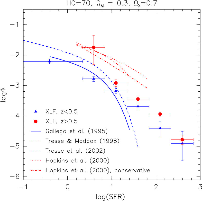
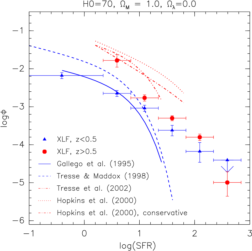
Figure 6.— Comparison of H$\alpha$ and X-ray luminosity functions (based on the combined CDF-N and CDF-S Bayes-selected sample as shown in Figure 3) after both have been rescaled to star-formation rates. The H$\alpha$ points were taken from Tresse et al. (2002, z $\sim$ 0.7), and Schechter function fits to H$\alpha$ LFs were taken from Gallego et al. (1995, z $\sim$ 0.),Tresse, & Maddox (1998, z $\sim$ 0.3), and Hopkins, Connolly, & Szalay (2000, z $\sim$ 1.3). Note that Hopkins, Connolly, & Szalay (2000) included the H$\alpha$ data from Yan et al. (1999) in their fits. The H$\alpha$ data are listed in the legend in order of increasing redshift; the z $<$ 0.5 data and curves are plotted in blue and the z $>$ 0.5 data and curves are plotted in red. The curves are plotted only at the range in luminosity (and hence SFR) over which the fits were performed. The left panel shows the X-ray luminosity function calculated for the cosmology $H_{0}$ = 70 km s^-1 Mpc^-1, $\Omega_{m}=0.3$ and $\Omega_{\Lambda}=0.7$, and the published $H\alpha$ values were converted from the cosmologies used ($H_{0}$ = 50 km s^-1 Mpc^-1, $q_{0}$ = 0.5 in most cases) by scaling the luminosities by $D_{L}^{2}$ and the normalization by $dV_{c}/dz^{-1}$ evaluated at the mean redshift of each survey (see text for details). The right panel shows the XLF rebinned for a cosmology of $H_{0}$ = 70 km s^-1 Mpc^-1 and $q_{0}$ = 0.5, in which case the published H$\alpha$ LFs are simply rescaled by $H_{0}^{-2}$ in luminosity and $H_{0}^{3}$ in normalization. Both cases are shown here since the cosmology correction applied in the first case is only an approximation (out of necessity). Hopkins, Connolly, & Szalay (2000) gave two H$\alpha$ LFs based on a “conservative” sample where the H$\alpha$ emission was securely measured and a sample in which less secure H$\alpha$ line identifications were also considered (i.e., the “true” H$\alpha$ LF at this redshift is between these two extremes).

In Figure 6, the Schechter function fits to the H$\alpha$ LFs from Gallego et al. (1995), Tresse, & Maddox (1998), Hopkins, Connolly, & Szalay (2000), and Tresse et al. (2002) are shown. Note that the results of Yan et al. (1999) are consistent with those given in Hopkins, Connolly, & Szalay (2000) and were included in the Schechter function fits in Hopkins, Connolly, & Szalay (2000). The H$\alpha$ luminosities are converted to a SFR function by multiplying the $H\alpha$ luminosities by $7.9\times 10^{-42}\rm M_{\odot}\ yr^{-1}\ ergs^{-1}\ s$ (Kennicutt, 1998). The XLF based on the combined CDF-S + CDF-N Bayes-selected sample shown in Figure 3 was converted by multiplying the X-ray luminosities by $2.2\times 10^{-40}\rm M_{\odot}\ yr^{-1}\ ergs^{-1}\ s$ (RCS). Note that the extinction-corrected z $\sim$ 0.7 H$\alpha$ LF overlaps with the uncorrected z $\sim$ 1.3 LF, implying that the extinction correction (a factor of $\sim$ 2) is of the same order as the evolution in the H$\alpha$ LF between these redshifts.

The most striking feature of the XLF / H$\alpha$ LF comparison is that the two sets of luminosity functions have different shapes, and more specifically different bright-end slopes. As with the FIR comparison the XLF data prefer a flatter bright-end slope than is the case in the H$\alpha$ Schecter function fits. The bright-end of the Schechter function is an exponential cut-off, and therefore the only “tuning” that can be done to fit the bright end of the LF is adjusting $L_{*}$. Accordingly the closest agreement in shape between the X-ray and H$\alpha$LFs is with the Hopkins et al. “conservative” Schechter fit, which had the largest value of L_∗. However, note that the shape of the H$\alpha$ LF fits should only be considered to be representative since the Schechter function fit parameters are not usually well constrained (and in addition are often correlated; see Hopkins et al. 2000). The relevance of the form of the luminosity functions is discussed below.

3.2. Towards a Physical Understanding of the Luminosity Functions associated with Massive Star Formation Indicators.

The galaxy luminosity functions for cosmic star formation indicators have either: (I) a Schechter distribution or (II) a lognormal distribution and we discuss each of them in turn below.

3.2.1 Schechter Distribution

.

The Schechter distribution was derived to fit the luminosity function for normal galaxies. It is associated with the hierarchical build up of luminous baryonic mass, in dark matter potential wells, to form the luminous galaxy distribution function. It is obvious that if: (1) the initial stellar mass function(IMF) is approximately universal; (2) the (massive) star formation rate per unit luminosity is roughly constant and (3) the H$\alpha$ is not significantly obscured by dust then the H$\alpha$LF should roughly reflect the parent Schechter LF of the galaxies.

3.2.2 Lognormal Distribution

Lognormal distributions are associated with physical systems that depend on many random multiplicative processes (and many associated random multiplicative probability distributions). A good example is the complex physics leading to relatively simple and robust probability density functions in a multi-phase,turbulent self-gravitating system (Wada & Norman, 2001). It is not surprising a lognormal distribution results for complex star forming systems with,for example, either:(1) reprocessing of the radiation by dust into the IR,to make the IRLF or;(2) evolutionary processes of massive stars in binaries accreting matter to produce the X-rays of the XLF. One way to think of this is to imagine, for example in the x-ray binary emission case, all the time ordered processes that a piece of matter undergoes on its way to emit an X-ray photon from accretion processes onto compact objects in binary systems. Subsequently, the photon may also be reprocessed on its way to the observer. To make this argument more explicit let us assume that the Schechter function discussed above for the H$\alpha$LF is dependent on the variable X(SH$\alpha$) given by:

$$X(SH\alpha)=x(star)x(IMF)x(U)x(f_{B})=\prod_{i=1}^{4}x(i)$$ (3)

where the four x(i) functions on the right are related to star formation, the IMF, the cosmological parameters including $\Omega_{m}$, and the baryonic fraction respectively. This schematic model is meant to indicate that the H$\alpha$LF depends on a few variables.

The physics behind the production of X-ray luminosity are more complicated. For example for the X-ray luminosity variable X(xray) we could write:

X(xray) = X(SH$\alpha$) x(binary) x(compact) x(high mass) x (accretion) x(metallicity) x(HI)… = $\prod_{i=1}^{N}x(i)$

where here the, N, x(i) functions on the right side depend not only on the four x(i) variables that we have included in our schematic representation of the Schecter $H\alpha$ LF but on a total of, N, x(i) functions describing the formation of binaries, compact objects in the binaries, high mass companions, physics of accretion, metallicity and HI column … respectively. Here, the point is that the production of X-rays depends on many more variables, $N>>1$, in an approximately multiplicative fashion. Consequently, the natural distribution for large N multiplicative variables is the lognormal.

Similar ideas apply to the IRLF where, again, we can write:

X(IR) = X(SH$\alpha$) x(dust) x(transfer) x(metals) x(SN:dest/form) x(molcloud) x(m,i) x(dyn)…

= $\prod_{i=1}^{N}x(i)$

where again we have, in addition to the basic Schecter variables, additional x function variables describing the physics of dust, radiative transfer, supernovae destruction and formation of grains, the molecular environment, the triggering of star formation by mergers and interactions and other dynamical instabilities (such as bars, and oval distortions).. respectively.

In summary, our argument is that the lognormal distributions, such as the IRLF, XLF and RadioLF are functions of many complicated physical processes, as discussed above, and the Schechter type functions, such as the H$\alpha$LF and the K-band LF depend on relatively simple and relatively few processes.

3.2.3 Future Work

Detailed models could be developed using the ideas discussed above but with more attention to the detailed physical processes. Possibly, the lognormal distributions may be associated more with starbursting normal galaxies rather than normal quiescent galaxies. It is likely that starbursting events are triggered in some way, by external galaxy merging and interactions or by internal dynamical instabilities such as bar formation. The random nature of such triggering processes may naturally lead to the type of multiplicative probability chain that would produce lognormal distributions. The more normal star formation mode may be reflected by the H$\alpha$. It would then be very interesting that normal modes and the triggered modes contribute very roughly the same amount of the cosmic SFR. For a detailed discussion of the merits of H$\alpha$ versus IR star formation rate indicators see Kewley et al. (2002).

4. Cosmic Star Formation History

In Figure 7 we show the cosmic star formation history taken from Tresse et al. (2002), with X-ray points added at z=0.27 and z=0.79 based on the combined CDF-N+S Bayes sample. We chose the Bayes sample since the XLF is in better agreement with the FIR prediction (see below). We computed the X-ray luminosity density by integrating $\Phi(logL)LdlogL$ and rescaling by $2.2\times 10^{-40}\rm M_{\odot}\ yr^{-1}\ erg\ s^{-1}$ (RCS). This resulted in SFR density estimates of $2.0\times 10^{-2}$ and $6.0\times 10^{-2}\ \rm M_{\odot}\ yr^{-1}Mpc^{-3}$ at two redshifts.

Figure 7.— Compilation of SFR densities from Tresse et al. (2002), including the X-ray points for z=0.27 and z=0.79 from this work. The X-ray points are shown with black filled squares. The triangles represent the H$\alpha$ SFR values from Gallego et al. (1995) at z $\sim 0$, Gronwall (1999) at z$\sim 0.05$, and Hopkins, Connolly, & Szalay (2000) at z$\sim 1.3$. The empty square represents the UV-selected H$\alpha$ Pascual et al. (2001) value at z$\sim 0.24$. The filled circles show the SFR densities from Tresse et al. (2002). The star gives the UV-selected z=0.15 SFR density from Sullivan et al. (2000). The open circles give 2800Å  CFRS points from Lilly et al. (1996), without dust correction. We also plot the SFR history based on the 60 $\mu$m LF luminosity density at z $\sim 0$, including (1+z)³ evolution. The 60 $\mu$m luminosity density was computed from Saunders et al. (1990, solid line) and Takeuchi, Yashikawa, & Ishii (2003, dotted line).

Note that the integration of an LF tends to be dominated by the contribution of the LF near L_∗. Here we primarily only sample galaxies brighter than L_∗, and therefore this estimate is a lower limit to the true SFR. However we also integrated the rescaled FIR LF (the curves in Figure 3b including k-corrections) at those redshifts, resulting in SFR = 0.022 and 0.055 $\rm M_{\odot}\ yr^{-1}Mpc^{-3}$. The two approaches resulted in consistent SFR estimates however the errors are large on the XLF data points, particularly on the lowest luminosity points which dominate the luminosity density sum. Therefore, we estimated the error on the SFR by summing the upper and lower error bounds on the XLF data points. This resulted in errors in log SFR of $\sim 0.16$ and $\sim 0.31$ at z=0.27 and 0.79, respectively. In this figure the SFR density estimates from Tresse et al. (2002) were corrected to $h=0.7,\Omega_{\lambda}=0.7,\Omega_{M}=0.3$.

The X-ray SFR points are consistent with an evolution of the SFR for $0<z<1$ of SFR $\propto(1+z)^{2.7}$ (i.e., an increase by a factor of $\sim 2.5$ in SFR density between z $\sim 0.3$ and z $\sim 0.8$). The Tresse et al. SFR history plot includes UV and extinction-corrected H$\alpha$ values. The z $\sim 0.3$ XLF SFR estimate is more consistent with the H$\alpha$ SFR estimate and the z $\sim 0.8$ XLF SFR estimate is intermediate between the H$\alpha$ and UV SFR values. However since the error on the z $\sim 0.8$ XLF SFR is large it is consistent with either the UV or H$\alpha$ SFR. We also plotted the z $\sim$ 0 SFR predicted from the Saunders et al. (1990) 60 $\mu$m LF (solid line) with an evolution of $(1+z)^{3}$, as well as the 60 $\mu$m SFR predicted by integrating the 60 $\mu$m LF in Takeuchi, Yashikawa, & Ishii (2003, dotted line). In both cases the 60 $\mu$m/SFR conversion of $2.6\times 10^{-10}\ M_{\odot}\ \rm yr^{-1}[L_{60}/L_{\odot}]^{-1}$ (where $L_{60}/L_{\odot}$ is the 60 $\mu$m luminosity in solar units) from Rowan-Robinson et al. (1997) was used. The Takeuchi, Yashikawa, & Ishii (2003) 60 $\mu$m LF has a somewhat steeper faint-end slope, which resulted in a factor of $\sim 2$ larger luminosity density.

5. Discussion

Our studies have focused on establishing the X-ray derived cosmic star formation rate and the normal star-forming galaxy X-ray Luminosity functions up to redshifts of order unity. Mild evolution is seen. The results presented here open up a new waveband for such star formation studies with the significant advantage that obscuration effects are not present. The Bayesian techniques developed in this paper for the galaxy selection have a wide range of applicability for further such studies. We now discuss important aspects of our results in more detail below.

5.1. Normal Star-Forming Galaxy X-ray Luminosity Functions

We have derived the first X-ray galaxy luminosity functions at the redshifts of $\sim 0.3$ and $\sim 0.7$. The high-luminosity bins for both the z$<$0.5 and z$>$0.5 Bayesian sample XLFs tend to be flatter than the predictions based on rescaling the FIR LF, although there is better agreement when the XLF is compared to the “warm” galaxy FIR LF rather than the full PSCz sample FIR LF. This implies that there is some AGN contamination in the sample. The spectroscopic CDF-S sample XLF also appears to be somewhat flat, which may indicate that absorbed and/or low-luminosity AGN are being missed in the optical spectra, although the small number of galaxies in that sample results in large statistical errors. Near IR spectra may be more revealing (e.g., Veilleux, Sanders & Kim, 1999). This overall agreement with the FIR prediction suggests that X-rays may be a useful tool for discriminating AGN2 and galaxies in surveys, due to the ability of X-rays to penetrate columns of $10^{22-23}\ \rm cm^{-2}$ as typically observed in Compton-thin AGN2. Finally, $\log L_{X}<40.5$ bin from the Bayesian z $<$ 0.5 XLF is most consistent with the local (full sample) FIR LF and the z=0 XLF from Schmidt, Boller, & Voges (1996), implying no evolution. However the mean redshift of galaxies with $\log L_{X}<40.5$ is only 0.16, implying evolution only on the order of $\sim 50\%$ in luminosity.

5.2. Star Formation Rates from X-ray Studies

Detailed physical modeling of the X-ray emission from galaxies and its application in measuring cosmic star formation history has been considered recently by Cavaliere, Giacconi & Menci (2000) for the hot gas component, Ghosh & White (2001) and Ptak et al. (2001) for the X-ray binary component, and for high mass binaries by Grimm, Gilfanov & Sunyaev (2003). The spectral energy distribution (SED) for starburst galaxies has been modeled by Persic & Rephaeli (2002). The potentially dominant contribution from Ultra-Luminous X-ray point sources (ULXs) has been analyzed in a recent paper by Colbert et al. (2003).

The physical reason for the correlation of both hard and soft X-ray luminosity with SFR is worth studying because it seems to constrain the overall physics of massive star formation and evolution. One possibility is that the (accretion-powered) core-collapse supernovae provide the hot $1$ keV component and the accretion-powered high-mass X-ray binaries dominating the point source contribution (Grimm, Gilfanov & Sunyaev, 2003). However, the detailed physics of how the relative branching ratios to SNe and to HMXBs for the evolution of the massive star population can conspire to produce the flat SED is not yet clear. We argue below that not only must the single star IMF be fixed but the bivariate binary star IMF($M_{1},M_{2}$) must also be approximately constant. For a flat SED, what is required is that the massive stars ending in Type II SNe powering the 1 keV hot gas component of the ISM and the HMXBs for the evolution of massive stars in binaries must be giving approximately equal energy per octave. Detailed studies of nearby galaxies and detailed population synthesis models help significantly (Zezas & Fabbiano, 2002; Georgantopoulos, Zensas & Ward, 2003; Swartz et al., 2003; Colbert et al., 2003; Sipior et al., 2003). In general, the X-ray luminosity of a galaxy can be related to the mass of the galaxy, $M$ and its star formation rate, $SFR$ by :

$$L_{X}=\eta_{M}M_{G}+\eta_{*}{\dot{M}_{*}}$$ (4)

where the $\eta$’s are linear efficiency factors. The first term is due to the old low mass X-ray binary population(LMXBs) and the second term is due to the high mass binaries (HMXBs) and the hot gas powered by SNe. In the Chandra band (0.3-8 keV), the X-ray point-source luminosity is proportional to the mass and SFR with coefficients $\eta_{M}=1.3\times 10^{29}\rm\ ergs\ s^{-1}\ M_{\odot}^{-1}$ and $\eta_{*}=0.7\times 10^{39}\rm\ ergs\ s^{-1}\ (M_{\odot}\ yr^{-1})^{-1}$ (Colbert et al., 2003). In the soft band (0.5-2.0 keV) the star formation dominates for galaxies with $L_{X}\gtrsim 10^{39}\ \rm\ ergs\ s^{-1}$ (as indicated in X-ray observations of the composite emission of starburst galaxies; Dahlem, Weaver & Heckman (1998); Ptak et al. (1999)). It was, therefore, not surprising that Ranalli, Comastri & Setti (2003) found that the soft X-ray luminosity of starburst galaxies is proportional to the SFR alone, specifically with $\eta_{M}\sim 0$ and $\eta_{*}=4.5\times 10^{39}\rm\ ergs\ s^{-1}\ (M_{\odot}\ yr^{-1})^{-1}$.

The extinction-corrected H$\alpha$ star formation history and the X-ray star formation history formally agree within the errors, although the X-ray SFR values are lower than the H$\alpha$ SFR values. This is probably due in part to the different sample selection and the different corrections applied to calculate the SFR. The revision to the 60 $\mu$m LF given in Takeuchi, Yashikawa, & Ishii (2003) resulted in a factor of $\sim 2$ increase in the 60 luminosity density relative to the value given in Saunders et al. (1990). It is likely that future work on both the H$\alpha$ LF and XLF will similarly result in adjustments to the SFR estimates.

The recent comprehensive study of Cohen (2003) using spectroscopy of the [OII]3727 $\AA$ line emitted by galaxies found in the 2 Ms exposure of the CDF-N shows that the $L_{X}$-SFR rate is similar locally and at redshifts of order unity, which is consistent with what we assume here.

The basic ingredients of a workable model are fairly clear:

(1)Constant IMF($M_{1},M_{2}$).

A constant two-parameter IMF(B($M_{1}$, $M_{2}$),S($M_{1}$))for binary stars(B) and single stars(S) as a function of $M_{1}$ and $M_{2}$. This is probably an important implication of the work of Ranalli, Comastri & Setti (2003) and if the general consistency here between the x-ray star formation results and the star formation indicators.

(2)Normal Stellar Evolution and Binary Star Evolution.

Straightforward stellar evolution and binary evolution to produce roughly constant branching ratios for high-mass X-ray binaries (HMXB) and core collapse SNeII. This is probably satisfied since we expect no surprises in stellar evolution and binary evolution (Ghosh & White, 2001).

(3)Consistent ISM properties.

It is also necessary to have at least very roughly constant properties for the interstellar medium(ISM). Over the whole galaxy ensemble, no large variations in the properties of the ISM including: dust-to-gas ratio, grain properties, metallicity, dense molecular environments and galactic winds. However, the dispersion of ISM properties from galaxy-to-galaxy is known to be large. For example, there are large well-known variations in the grain properties in the LMC, the SMC and the Galaxy.

(4)Consistent Dynamical Properties.

The population of normal starbursting galaxies we are studying can have additional dynamical and environmental constraints due to the amount of merging, interactions, barred driven inflow…

The first two points (1,2) give a way to understand the rough correlations and the last two points (3,4) give the dispersion and the overall lognormal shape to the radio, IR and X-ray LFs.

The star formation history derived from the X-ray data using the empirically derived relation between X-ray luminosity and star formation rate from Ranalli, Comastri & Setti (2003) is in rough agreement with other methods although, as discussed by Hogg (2004) there is a large dispersion in the results.

5.3. Hidden Active Galactic Nuclei

An important issue is whether the X-ray emission from our galaxies could be due to central AGNs hidden in faint Type 2 Seyfert nuclei lurking in the center of our galaxies Moran, Filippenko & Chornok (2002). This is not likely because Seyfert 2s have a hard spectrum with hardness ratio $HR>0$, whereas the galaxies in our sample have softer spectra.

A key advantage to using soft X-ray luminosities to estimate the X-ray galaxy luminosity function and the SFR is that the soft band tends to be dominated by starburst emission regardless of whether an obscured AGN is present (see, e.g., Turner et al., 1997; Levenson, Weaver, & Heckman, 2001). This assists us in discerning galaxies from AGN2.

5.4. Implications for Future X-ray Missions

Our cosmological star formation studies, extending up to $z\approx 1$, require the combination of 1-2 Msec $Chandra$ exposures and high-quality optical spectroscopic coverage from large-aperture ground-based telescopes such as VLT and Keck. There is, however, a wealth of information on galaxy evolution available through current ground-based wide-field optical surveys (e.g., 2dF and SDSS) that is still relatively underutilized. The small fields of view of $Chandra$ and $XMM$-$Newton$ make X-ray studies of these wide-field galaxy surveys quiet difficult (but see e.g., Georgakakis et al., 2003, for an example of one high-quality statistical study of 2dF galaxies with $XMM$-$Newton$). Deeper wide-field X-ray surveys would also be complementary to the deep wide-field ultraviolet imaging surveys of GALEX. The GALEX surveys, currently underway, are probing star formation from $z=0-2$, overlapping with the work we present here. Possible future wide-field X-ray telescopes include the Wide Field X-ray Telescope (WFXT) Burrows, Burg & Giacconi (1992) and its successors WAXS/WFXT (Chincarini et al., 1998) and DUET (Jahoda et al. 2003).

X-ray studies of galaxies may be extended to truly extreme redshifts when high-sensitivity X-ray telescopes such as XEUS (Parmar et al., 2003) commence operation. XEUS may achieve sensitivities as faint as $4\times 10^{-18}$ erg cm^-1 and at this level galaxies will dominate the X-ray source number counts. This sensitivity will allow for the detection of star-forming galaxies to great distances ($z>5$) and will allow for the probing of X-ray emission from star formation to the very epoch of galaxy formation in the early Universe.

6. Conclusions

There are five main conclusions of this work.

1. We have established the X-ray luminosity functions of galaxies in the Chandra deep Fields North and South. These XLFs have a lognormal distribution. The XLFs are completely consistent with both the infra-red luminosity functions (IRLFs) and the GHz radio luminosity functions(RLFs), which both have lognormal distributions.

2. The evolution of the XLFs is consistent with a pure luminosity evolution(PLE) of $\sim(1+z)^{2.7}$.The more robust integral of the XLFs can be transformed to an x-ray derived cosmic star formation history. This cosmic star formation rate (SFR) is consistent with the (mild) evolution in SFR $\propto(1+z)^{2.7}$. In general, the overall SFR estimates in the range of redshift from unity to the present epoch show a wide scatter although there is a general trend of mild evolution consistent with the above. To reduce the scatter and better understand the evolution of the SFR in this redshift range one needs in the future:(1) more sensitive wide area studies such as the GALEX mission (2) extensive multi-band studies; the XLFs and X-ray derived SFRs now bring in a new waveband here and (3) deeper physical understanding of the star formation indicators.

3. The H$\alpha$LFs have the form of the Schechter luminosity function which fits the galaxy luminosity functions in J and K. The H $\alpha$ distribution is quite different from the the lognormal distributions for the XLF, IRLF and RLF discussed above. A detailed physical understanding is not yet available.

4. The X-ray derived star formation history gives an interesting constraint on the IMF. The X-ray emission in the Chandra band is most likely due to binary stars. The overall consistency and correlations between single star effects and binary star effects in different wavebands indicate that the bivariate IMF($M_{1},M_{2}$) must be universally constant, at least at the high mass end, since the X-ray observations may be measuring directly the binary star formation history of the Universe.

Appendix A Bayesian Statistical Analysis

For many of the sources in our sample both the X-ray and optical information is limited. Classifying a source based simply on “sharp” cuts in parameter space, such as log $L_{X}<42\ \rm ergs\ s^{-1}$ and X-ray hardness HR $<-0.2$, does not take into account the errors in the measured quantities and the fact that the parent distribution (i.e., real galaxies in the Universe) are not so sharply delineated. Here we remedy this situation by using a Bayesian statistical approach. Specifically, we assume parent distribution models for measured parameters, $\theta$, and then compute the conditional probability, $P_{M}$, of measuring the observed values of the parameters ($D$) by integrating over the parent distributions for a given model M. Specifically, $\theta$ = {HR, $\log L_{X}$, $\log F_{X}/F_{opt}$}, where HR is the X-ray hardness ratio, $F_{X}$ is the 0.5-2.0 keV luminosity, and $\log F_{X}/F_{opt}$ is the X-ray/optical flux ratio. $\log F_{X}/F_{opt}$ is given by $\log_{10}(F_{0.5-2.0\rm\ keV}-R/2.5-R_{0}$, where $R_{0}$ = 5.5 for CDF-N sources (Hornschemeier et al., 2003) and $R_{0}$ = 5.7 for CDF-S sources (Szokoly et al., 2004). $P_{M}$ is given by $P_{M}=\int p_{M}(\theta|D)d\theta$, with

$$p_{M}(\theta|D)=p_{M}(\theta)p(D|\theta)/p(D)$$ (A1)

$p(D|\theta)/p(D)$ is the probability of observing a given set of parameter values D when the expected (i.e., parent) values are $\theta$, which is simply the likelihood function for the data. In this analysis we assume that the errors on each parameter are reasonably approximately Gaussian, and defer the treatment of the more general likelihood functions for future work. $p_{M}$ is the prior, or parent population probability distribution for a sources of type M. We further assume that the parent distributions of the parameters are also reasonably approximated by a Gaussian, with the mean and standard deviations of the Gaussian set to the observed values for the parameter (see below). $p_{M}$ should be normalized by the relative number of sources of a given type that would be detected in the 0.5-2.0 keV bandpass. However, since these numbers are not known precisely and the relative number of sources used in the statistical analysis below are approximately equal, we set this term to unity here. Therefore $P_{M}$ is given by

$$P_{M}=\Pi_{i}\int d\theta_{i}\frac{1}{\sqrt{2\pi}\sigma_{i}}\exp[-\frac{(\theta_{i}-\bar{\theta_{i}})^{2}}{2\sigma_{i}^{2}}]\frac{1}{\sqrt{2\pi}\Delta x_{i}}\exp[-\frac{(x_{i}-\theta_{i})^{2}}{2\Delta x_{i}^{2}}]$$ (A2)

Here $\bar{\theta}_{i}$ and $\sigma_{i}$ are the parent distribution mean and standard deviation for the ith parameter, while $x_{i}$ and $\Delta x_{i}$ are the measured value and error for that parameter. For more discussion of Bayesian methods used in model testing, see Hobson & McLachlan (2003) and references therein.

Applying these methods to our sample, we have chosen Gaussian parent distribution functions whose mean and standard deviations ($\sigma$) are derived from the subset of X-ray sources which have high-quality optical spectroscopic identifications (Szokoly et al., 2004). We further require that the sources have constrained hardness ratios (relevant mostly for the galaxies, which were X-ray faint) when computing the mean and standard deviation of the hardness ratios. The histograms of the observed parameters are shown in Figures 8-10. The Gaussian parameters are shown in Table 1 and the corresponding Gaussian curve is also plotted in Figures 8-10.

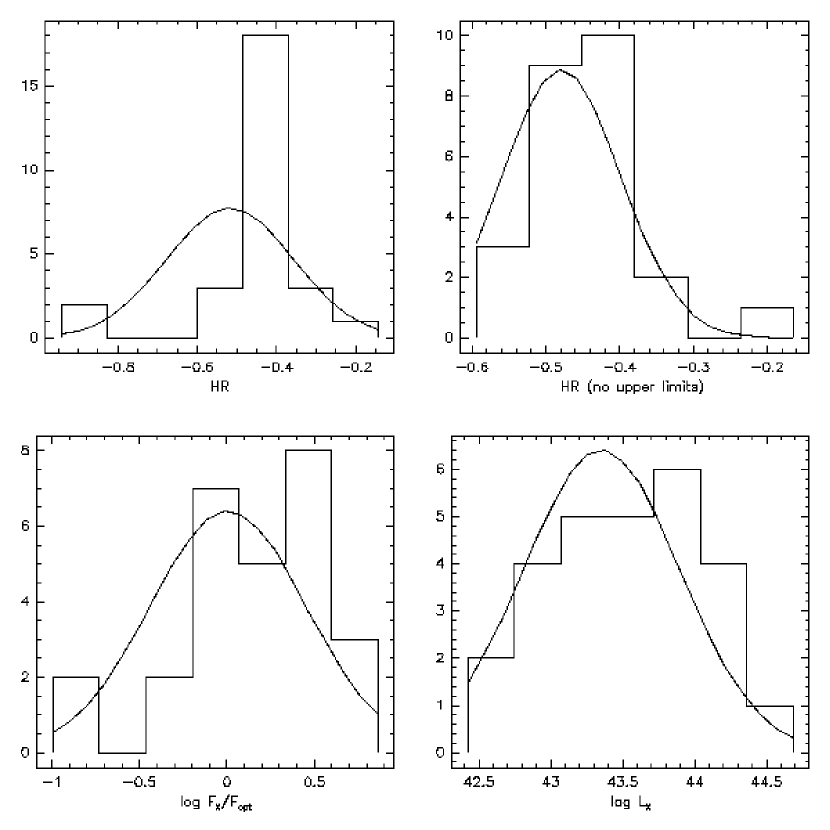
Figure 8.— The observed parameter distributions for AGN1 sources in the CDF-S. The y-axes are numbers of sources. The curves show the Gaussian resulting from taking the mean and standard deviation of the distribution.

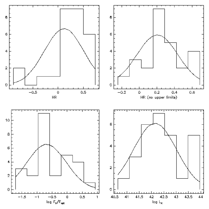
Figure 9.— As in Figure 8, except for AGN2 sources.

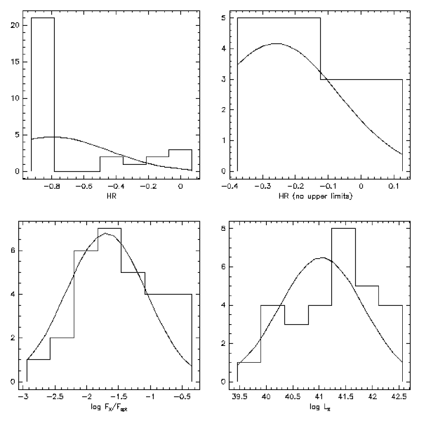
Figure 10.— As in Figure 8, except for galaxy sources.

Table 1Statistical Parameters for the Galaxy, AGN1 and AGN2 CDF-S Samples

Source Type	Number	$\bar{\log L_{X}}$	$\sigma_{\log L_{X}}$	$\bar{HR}$	$\sigma_{HR}$	$\bar{\log F_{X}/F_{opt}}$	$\sigma_{\log F_{X}/F_{opt}}$
Galaxy	8/29	41.0	0.8	-0.26	0.19	-1.7	0.6
AGN1	25/27	43.4	0.5	-0.48	0.08	0.0	0.4
AGN2	26/28	42.1	0.9	0.21	0.23	-0.7	0.6

Note. — The Number column lists the number of sources of the given type with a detection in the hard band / the total number of sources of that type. Sources with upper-limits on the hardness ratio (i.e., without hard band detections) were excluded when computing the mean and standard deviation of HR.

Using these assumed models, the observed errors on HR, and an assumed error of 0.25 on $\log L_{X}$ and $\log F_{X}/F_{opt}$, we computed the probability of each source being a galaxy, an AGN1 and an AGN2. Note that the errors on HR were also taken to be Gaussian, using the larger of the upper and lower error estimates (derived using Lyons, 1991; Kraft, Burrows, & Nousek, 1991, ; see discussion in Alexander et al. 2003). A source is classified as a given type when the computed probability for that type is the greatest. As a check, we summarize in Table 2 the results for the sources with high-quality classifications (i.e., those used to produce the parent distribution models as discussed above). Of course in general a control sample is necessary to properly assess the performance of a classification procedure, however our sample is too small to allow for this approach. However in future work this test will be performed with other data sets (most notably using GOODS data). As would be expected, nearly all of the false galaxy identifications were AGN2 and vice-versa.

Table 2Bayesian Classification Results

Source Type	Number	Galaxy	AGN1	AGN2
Galaxy	29	25	2	2
AGN1	27	1	25	1
AGN2	28	3	1	24

Note. — Source Type gives the spectroscopic classification of the sources.

Appendix B Galaxy Sample

In Table 3 we give the identification numbers (as given in Giacconi et al. 2002 and Alexander et al. 2003), redshift and $\log L_{X}$ values for the galaxies in the Bayesian-selected sample. The sources that are also in the spectroscopic CDF-S sample are marked. There are also 3 additional sources in the spectroscopic CDF-S sample that were not selected as galaxies by the Bayesian analysis, which have IDs 49, 242, and 519, redshifts 0.53, 1.03, and 1.03, and $\log L_{X}$ values 42.3, 42.3, and 41.9. As might be expected, these were the spectroscopic CDF-S sample galaxies with the highest $L_{X}$ values.

Table 3XLF galaxy sample

ID #a	$z$	$L_{X}$ (0.5–2 keV)
CDF-S sample:
1	0.347	41.73
12*	0.251	41.65
40	0.545	42.16
77	0.622	42.26
84	0.103	40.38
95	0.076	39.95
96	0.274	40.78
97	0.180	41.16
98	0.279	41.02
103	0.215	40.92
116	0.076	39.87
170	0.664	41.55
173*	0.524	40.92
175*	0.522	41.12
185	0.925	41.51
186	1.158	41.81
211	0.679	41.81
218	0.497	41.29
224*	0.738	41.77
229*	0.103	39.78
233*	0.577	41.01
236	0.731	41.68
246	0.690	41.98
247	0.040	38.64
249	0.964	41.85
504	0.541	41.53
509	0.556	41.59
511	0.767	41.52
512*	0.668	41.52
514	0.103	39.63
516*	0.665	41.47
521*	0.131	39.94
525	0.229	40.49
534	0.676	41.03
535*	0.575	41.43
536	0.444	41.10
538	0.310	40.50
552	0.673	41.63
553	0.366	40.97
554	0.225	40.67
556	0.635	41.33
557	0.500	40.85
558	0.585	41.49
559	0.114	39.78
560*	0.669	41.36
565*	0.363	40.42
566	0.734	41.74
567*	0.456	40.81
573*	0.414	40.61
575*	0.340	40.45
577*	0.547	41.23
578	0.969	41.62
580*	0.664	41.13
581	0.799	41.44
582*	0.241	40.15
586*	0.580	41.05
587*	0.246	40.07
590	0.280	40.36
592	1.150	41.78
594	0.733	41.91
617	0.588	41.54
619	0.050	38.91
620*	0.648	41.15
621	0.290	40.30
624*	0.668	41.17
625	1.151	41.76
627*	0.248	40.12
628	0.200	39.98
629	0.410	40.71
644	0.119	40.08
646	0.438	40.79
650	0.223	40.67
651	0.182	40.57
652*	0.077	39.24

Table 4XLF galaxy sample

ID #a	$z$	$L_{X}$ (0.5–2 keV)	ID #a	$z$	$L_{X}$ (0.5–2 keV)
CDF-N sample:
3	0.138	40.29	6	0.135	40.83
22	0.317	39.89	46	0.207	40.43
49	0.296	41.27	55	0.637	41.30
56	0.108	39.77	57	0.375	40.87
60	0.529	40.78	62	0.087	38.70
66	0.333	41.24	67	0.639	41.39
69	0.520	41.11	78	0.747	41.66
81	0.409	40.77	87	0.136	39.76
93	0.275	42.08	101	0.454	40.81
103	0.969	42.13	105	0.319	39.99
111	0.515	40.64	114	0.534	40.63
119	0.473	40.83	120	0.694	41.27
121	0.520	41.33	126	0.779	40.91
131	0.631	40.62	132	0.647	41.07
136	0.472	40.65	138	0.483	40.79
141	0.746	41.87	148	1.130	41.96
166	0.455	40.50	169	0.845	41.53
175	1.014	41.99	177	1.016	42.14
180	0.456	41.24	189	0.410	41.01
192	0.680	40.80	197	0.081	38.92
200	0.971	41.31	203	1.143	41.27
207	0.300	41.04	209	0.510	41.36
210	0.848	41.50	211	0.846	41.35
212	0.943	41.77	214	1.144	41.37
215	1.006	41.17	218	0.089	39.31
219	0.845	40.96	224	0.700	41.92
225	0.290	40.30	227	0.556	40.64
230	1.011	41.62	234	0.454	40.85
241	0.851	41.83	244	0.971	41.36
245	0.321	39.90	249	0.475	41.30
251	0.139	39.59	255	0.113	40.31
256	0.593	41.09	257	0.089	38.92
258	0.752	40.96	260	0.475	40.72
264	0.319	40.26	265	0.410	40.74
269	0.358	40.36	274	0.321	40.92
279	0.890	41.07	280	0.850	41.12
282	0.202	39.87	285	0.288	41.03
288	0.792	41.49	291	0.517	40.59
294	0.474	41.42	295	0.845	41.31
296	0.663	41.11	300	0.137	39.54
305	0.299	40.15	308	0.515	40.53
310	0.761	40.91	311	0.914	41.33
313	0.800	41.30	316	0.231	40.32
320	0.956	41.38	326	0.359	40.30
327	0.913	41.16	332	0.561	40.70
333	0.377	41.62	337	0.902	41.04
339	0.253	39.95	346	1.017	40.98
351	0.940	41.59	353	0.422	40.80
354	0.568	41.05	355	1.027	41.77
356	0.956	42.20	358	0.907	41.86
359	0.902	41.62	378	1.084	41.40
383	0.105	39.18	387	1.081	41.70
388	0.559	41.05	389	0.557	40.78
392	0.411	40.51	395	0.411	40.77
401	0.935	41.51	404	0.104	39.26
407	1.200	41.94	410	0.113	39.30
414	0.800	41.46	415	0.116	39.60
418	0.279	40.35	425	0.214	40.11
426	0.159	39.75	428	0.298	40.47
433	1.022	41.64	435	0.201	39.99
436	0.189	40.38	438	0.220	40.46
443	0.231	40.69	446	0.410	40.56
450	0.935	41.74	453	0.838	42.11
454	0.458	41.48	458	0.069	39.55
460	1.084	42.17	462	0.511	40.44
466	0.440	40.81	469	0.188	40.09
471	1.170	41.90	476	0.475	40.95
480	0.456	41.19	489	1.024	42.24

References

- Avni & Tannenbaum (1986) Avni, Y. & Tannenbaum, H. 1986, ApJ, 305, 83
- Alexander et al. (2003) Alexander, D.M. et al. 2003,AJ, 126, 539
- Alexander et al. (2002) Alexander, D.M. et al. 2002, ApJ, 568, L85
- Baldry et al. (2002) Baldry, I. K., et al. 2002, ApJ, 569, 582
- Barger et al. (2003) Barger, A.J., et al. 2003, AJ, 126, 632
- Barger et al. (2002) Barger, A.J., et al. 2002, AJ, 124, 1839
- Bauer et al. (2002) Bauer, F.E., Alexander, D.M., Brandt, W.N., Hornschemeier, A.E., C. Vignali, Garmire, G.P. & Schneider, D.P. 2002, AJ, 124, 2351
- Brandt et al. (2001) Brandt, W. N. et al. 2001, AJ, 122, 2810
- Burrows, Burg & Giacconi (1992) Burrows, C.J., Burg, R. & Giacconi, R. 1992 ApJ, 392, 760
- Cavaliere, Giacconi & Menci (2000) Cavaliere, A., Giacconi, R. & Menci, N. 2000 ApJ, 528, L77
- Chary & Elbaz (2001) Chary, R. & Elbaz, D. 2001, ApJ, 556, 562
- Chincarini et al. (1998) Chincarini, G., Citterio, O., Conconi, P., Ghigo, M. & Mazzoleni, F. 1998 Astron. Nachr., 319, 125
- Cohen (2003) Cohen, J. 2003, astro-ph/0307537
- Colbert et al. (2003) Colbert, E., Heckman, T., Ptak, A., Strickland, D., & Weaver, K 2003, ApJ, in press, astro-ph/0305476
- Cole et al. (2001) Cole, S. et al. 2001, MNRAS, 326, 255
- Condon, Cotton & Broderick (2002) Condon, J., Cotton, W. & Broderick, J. 2002, ApJ, 124, 675
- (17) Cowie, L.L., Songaila, A. & Barger, A.J. 1999 ApJ, 118, 603
- Dahlem, Weaver & Heckman (1998) Dahlem, M., Heckman, T.M.& Weaver, K.A. 1998 ApJS, 118, 401
- Fabbiano (1989) Fabbiano, G. 1989, ARA&A,27, 87
- Flores et al. (1999) Flores et al. 1999, ApJ, 503, 148
- Gallego et al. (1995) Gallego, J., Zamorano, J., Aragon-Salamanca, A. & Rego, M. 1995 ApJ, 459, L43
- Gehrels (1986) Gehrels, N. 1986, ApJ, 303, 336
- Georgantopoulos, Zensas & Ward (2003) Georgantopoulos, I., Zezas, A. & Ward, M.J. 2003ApJ, 584, 129
- Georgantopoulus, Basilakos & Plionis (1999) Georgantopolous, I., Basilakos, S. and Plionis, M. 1999 MNRAS, 305, L31
- Georgakakis et al. (2003) Georgakakis, A. et al. 2003, astro-ph/0305278
- Ghosh & White (2001) Ghosh, P. & White, N. 2001, ApJ, 559, L97
- Giacconi et al. (2002) Giacconi, R., et al. 2002, ApJS, 139, 369
- Glazebrook et al. (1999) Glazebrook, K., Blake, C., Economou, F., Lilly, S. and Colless, M. 1999 MNRAS, 306, 843
- Grimm, Gilfanov & Sunyaev (2003) Grimm, H.-J., Gilfanov, M. & Sunyaev, R. 2003, MNRAS,339, 793
- Gronwall (1999) Gronwall, C. 1999, in Holt S., Smith E., eds, Proc. Conf. ’After the Dark Ages: When Galaxies were Young’ AIP, New York, p. 335
- Haarsma et al. (2000) Haarsma, D.A., Partridge, R.B., Windhorst, R.A. & Richards, E.A. 2000 ApJ, 544, 641
- Hammer et al. (1997) Hammer, F. et al. 1997 ApJ, 481, 49
- Hasinger (2003) Hasinger, G. 2003, to appear in “High Energy Processes and Phenomena in Astrophysics”, IAU Symposium 214, X. Li, Z. Wang, V. Trimble (eds), astro-ph/0301040
- Hobson, Bridle and Lahav (2002) Hobson, M.P., Bridle, S.L. & Lahav, O. 2002 MNRAS, 335, 377
- Hobson & McLachlan (2003) Hobson, M. & McLachlan, C. 2003, MNRAS, 338, 765
- Hogg et al. (1998) ogg, D.W., Cohen, J.G., Blandford, R.D. and Pahre, M.A. 1998, ApJ, 504, 622
- Hogg (2004) Hogg, D.W. 2004, PASP, submitted (astro-ph/0105280)
- Hopkins, Connolly, & Szalay (2000) Hopkins, A., Connolly, A., & Szalay, A. 2000, AJ, 120, 2843
- Hopkins et al. (2003) Hopkins, A.M., Miller, C.J., Nichol, R.C., Connolly, A.J., Bernardi, M., Gomez, P.L., Goto, T., Tremonti, C.A., Brinkmann, J., Ivezic, Z. & Lamb, D.Q. 2003 ApJ, 599, 971
- Hornschemeier et al. (2002) Hornschemeier, A. et al 2002 ApJ, 568, 82
- Hornschemeier et al. (2003) Hornschemeier, A.,Bauer, F.E., Alexander, D.M., Brandt, W.N., Sargent, W.L.W., Bautz, M.W., Conselice, C., Garmire, G.P., Schneider, D.P., & Wilson, G. 2003, AJ, 126, 575
- Jones & Bland-Hawthorn (2001) Jones, D.H. & Bland-Hawthorn, J. 2001 ApJ, 550, 593
- Jahoda et al. (2003) Jahoda, K. et al. 2003, AN, 324, 132
- Kennicutt (1983) Kennicutt, R. 1984, ApJ, 272, 54
- Kennicutt (1998) Kennicutt, R. 1998, ARA&A, 36, 189
- Kewley et al. (2002) Kewley, L., Geller, M., Jansen, R., & Dopita, M. 2002, AJ, 124, 6
- Kilgard et al. (2002) Kilgard, R.E., Kaaret, P. Kraus, M.I., Prestwich, A., Raley, M.T. & Zezas, A. 2002 ApJ, 573, 138
- Kraft, Burrows, & Nousek (1991) Kraft, R., Burrows, D., & Nousek, J. 1991, ApJ, 374, 344
- Lanzetta et al. (2002) Lanzetta et al. 2002 ApJ, 570, 492
- Levenson, Weaver, & Heckman (2001) Levenson, N. A., Weaver, K., & Heckman, T. 2001, ApJ, 550, 230
- Lilly et al. (1996) Lilly, S.J., Le Fevre, O., Hammer, F., Crampton, D. 1996 ApJ, 460, L1
- Lyons (1991) Lyons 1991, Data Analysis for Physical Science Students (Cambridge: Cambridge Univ. Press)
- Madau et al. (1998) Madau, P., Ferguson, H., Dickinson, M., Giavalisco, M., Steidel. C. & Fruchter, A. 1996 MNRAS, 283, 1388
- Mobasher et al. (1999) Mobasher, B. et al. 1999 MNRAS, 308, 45
- Miley, Neugebauer & Soifer (1985) Miley, G.K., Neugebauer, G. & Soifer, B.T. 1985 ApJ, 293, L11
- Miyaji, Hasinger & Schmidt (2000) Miyaji, T., Hasinger, G. & Schmidt, M. 2000 A&A, 353, 25
- Miyaji, Hasinger & Schmidt (2001) Miyaji, T., Hasinger, G. & Schmidt, M. 2001 A&A, 369, 49
- Miyaji & Griffiths (2002) Miyaji, T. & Griffiths, R. ApJ, 564, 5
- Moran, Filippenko & Chornok (2002) Moran, E.C., Filippenko, A.V. & Chornok, R. 2002 ApJ, 579, L71
- Page & Carrera (2000) Page, M.J. & Carrera 2000 MNRAS, 311, 433
- Parmar et al. (2003) Parmar, A. et al., 2003, SPIE, 4851, 304
- Pascual et al. (2001) Pascual, S., Gallego, J., Aragon-Salamamca, A., & Zamorano, J. 2001, A&A, 379, 798
- Persic & Rephaeli (2002) Persic, M. & Rephaeli, Y. 2003 A&A, 382, 843
- Ptak et al. (1999) Ptak, A., Serlemitsos, P., Yaqoob, T. & Mushotzky, R. 1999 ApJS, 120, 179
- Ptak et al. (2001) Ptak, A., Griffiths, R., White, N. & Ghosh, P. 2001, ApJ, 559, L91
- Ranalli, Comastri & Setti (2003) Ranalli, P., Conmastri, A. & Setti, G. 2003 A&A, 399, 39
- Rola, Terlevich & Terlevich (1997) Rola, C.S., Terlevich, E. & Terlevich, R. 1997 MNRAS, 289, 419
- Rosati et al. (2002) Rosati, P., et al. 2002, ApJ, 566, 667
- Rowan-Robinson et al. (1997) Rowan-Robinson et al. 1997, MNRAS, 289, 490
- Santiago & Strauss (1992) Santiago, B. & Strauss, M. 1992, ApJ, 387, 9
- Saunders et al. (1990) Saunders, W., Rowan-Robinson, M., Lawrence, A., Efstathiou, G., Kaiser, N., Ellis, R.S. & Frenk, C.S. 1990 MNRAS,242, 318
- Schmidt (1968) Schmidt, M. 1968 ApJ, 151, 393
- Schmidt, Boller, & Voges (1996) Schmidt, K.-H., Boller, Th., & Voges, W. 1996, MPE Report, 263, 395
- Sipior et al. (2003) Sipior, M.S., Eracleous, M. amd Sigurdsson, S. 2003 astro-ph/0308077
- Sullivan et al. (2000) Sullivan, M., Treyer, M., Ellis, R., Bridges, T., Milliard, B., & Donas, J. 2000, MNRAS, 312, 442
- Sullivan et al. (2001) Sullivan, M., Mobasher, B., Chan, B., Cram, L., Ellis, R., Treyer, M. & Hopkins, A. 2001 ApJ, 558
- Sullivan et al. (2004) Sullivan, M., Treyer, M.A., Ellis, R.S. & Mobasher, B. 2004, MNRAS, in press (astro-ph/0310388)
- Swartz et al. (2003) Swartz, D.A., Ghosh, K.K., McCollough, M., Pannuti, T.G., Tennant, A.F. & Wu, K. 2003 ApJS, 144, 213
- Szokoly et al. (2004) Szokoly, G. P., et al. 2004, submitted, astro-ph/0312324