A Deep Chandra Observation of the Distant Galaxy Cluster MS1137.5+6625

Abstract

We present results from a deep Chandra observation of MS1137.5+66, a distant (z=0.783) and massive cluster of galaxies. Only a few similarly massive clusters are currently known at such high redshifts; accordingly, this observation provides much-needed information on the dynamical state of these rare systems. The cluster appears both regular and symmetric in the X-ray image. However, our analysis of the spectral and spatial X-ray data in conjunction with interferometric Sunyaev-Zel’dovich effect data and published deep optical imaging suggests the cluster has a fairly complex structure. The angular diameter distance we calculate from the Chandra and Sunyaev-Zel’dovich effect data assuming an isothermal, spherically symmetric cluster implies a low value for the Hubble constant for which we explore possible explanations.

1 Introduction

Rich galaxy clusters are useful cosmological probes. The richest clusters are thought to be massive enough to comprise a fair sample of the Universe, i.e., their mass composition should reflect the universal mass composition (White et al. 1993; Evrard 1997) and so provide an efficient laboratory for measuring the baryonic to dark matter ratio. The mere existence of massive galaxy clusters at high redshifts can also place powerful constraints on the physical and cosmological parameters of structure formation models (e.g., Peebles et al. 1989; Bahcall & Cen 1992; Luppino & Gioia 1995; Oukbir & Blanchard 1997; Bahcall & Fan 1998; Donahue et al. 1998; Eke et al. 1998; Haiman et al. 2001; Holder et al. 2001). The greatest leverage is provided by the most massive and distant clusters; in fact, to constrain $\Omega_{\Lambda}$ one must use clusters with redshifts greater than 0.5 (e.g., Oukbir & Blanchard 1997; Holder et al. 2001). For these reasons, we are particularly interested in observations of massive galaxy clusters at high redshift.

A set of observations of distant clusters can be used to constrain the expansion rate and curvature of the universe. The most noted approach is through the angular diameter distance relation. The theoretical value of the angular diameter distance $D_{A}(z)$ is cosmology-dependent; $D_{A}(z)$ can be calculated from measurements of the X-ray temperature and surface brightness profile of a cluster’s intracluster medium (ICM) analyzed in conjunction with a measurement of the cluster’s Sunyaev-Zel’dovich effect (cf. Birkinshaw et al. 1991; Birkinshaw & Hughes 1994; Myers et al. 1997; Hughes & Birkinshaw 1998; Reese et al. 2000; Patel et al. 2000; Grainge et al. 2002), a spectral distortion of the cosmic microwave background (CMB) radiation by the hot, ionized ICM (Sunyaev & Zel’dovich 1970, 1972).

Another approach to measuring cosmological constants with clusters uses the idea that the fraction of the total cluster mass contained in this atmosphere, the gas mass fraction $f_{g}$, traces the universal baryonic mass fraction, under the fair sample assumption. The fair sample assumption then implies also that the gas mass fraction in massive clusters should not vary.

With a well-chosen sample which includes clusters at high-redshifts, both the above determinations of the cluster gas mass fraction (cf. Sasaki 1996; Pen 1997; Rines et al. 1999) and cluster distances can be used to constrain the geometry of the universe, since at high redshifts, the calculated cluster distances and gas mass fractions depend significantly on the cosmological parameters $\Omega_{M}$ and $\Omega_{\Lambda}$. Recent measurements of $D_{A}(z)$ via the X-ray/SZE method (Mason et al. 2001; Reese et al. 2002; Jones et al. 2003) and of the gas mass fraction (Grego et al. 2001) in samples of clusters imply values of the Hubble constant and the curvature of the universe in good agreement with the values determined independently with other methods. In the work of Reese et al. (2002), the angular diameter distance to 18 clusters, distributed widely in redshift, is calculated. For $\Omega_{M}$=0.3, $\Omega_{\Lambda}$=0.7, they find the mean Hubble constant for the sample is 60${}^{+4}_{-4}\ {}^{+18}_{-13}$ km s^-1 Mpc^-1. For seven low-redshift clusters, Mason et al. (2001) find a mean Hubble constant of 66${}^{+14}_{-11}\pm$15 km s^-1 Mpc^-1 for this same cosmology. Jones et al. (2003) find a mean value of 65${}^{+8}_{-7}\pm$15 km s^-1 Mpc^-1 for five moderate-redshift clusters. (The uncertainties, statistical and systematic, are reported at 68% confidence.) These Hubble constant measurements agree within the uncertainties with the value derived from the Hubble Space Telescope $H_{\circ}$ Key Project (cf. Mould et al. 2000), 72$\pm 3\pm 7$ km s^-1 Mpc^-1, and Type Ia supernovae (cf. Riess et al. 1998), who find the Hubble constant to be $\sim$65, in the cosmology considered here.

When determining cosmological parameters from cluster distances and mass fractions, one generally assumes the dominant cluster physics is well-represented by a simple picture: galaxies and an ionized intra-cluster medium in hydrostatic equilibrium in a large dark-matter potential, supported by thermal pressure. In general, this is descriptive of clusters in the local universe, as evidenced by the strong correlations between X-ray luminosity and temperature (Mushotzky & Scharf 1997; Allen & Fabian 1998; Arnaud & Evrard 1999; Donahue et al. 1999) and cluster size and temperature (Mohr et al. 2000); and by the uniformity of the gas mass fraction in massive clusters (cf. David et al. 1995; Mohr et al. 1999). One can attempt to ameliorate the effects of departures from this simple picture on the accuracy of the results by determining cosmological parameters from samples of clusters, in which some of these systematic effects will average out, and taking care to choose the sample in an unbiased way. Indeed, much of the observational cluster work cited above (e.g., Mason et al. 2001; Grego et al. 2001; Reese et al. 2002) uses such an approach. In this work, we investigate the validity of the hydrostatic, isothermal, spherically symmetric assumption by studying observations of a massive (and therefore relatively bright) distant cluster.

We analyze a deep observation of the galaxy cluster MS1137.5+6625 taken with the Chandra Observatory’s Advanced CCD Imaging Spectrometer (ACIS). MS 1137.5+6625 was observed as part of L. VanSpeybroeck’s Cycle 1 Guaranteed Time Observations (GTO). These GTO observations, together with observations in subsequent Chandra observation cycles, form a collection of X-ray observations of galaxy clusters designed for measuring cosmological parameters to high accuracy. Over 1,250 ks of Chandra time were scheduled for this project in observation Cycles 1 and 2, and it included over 40 clusters by the close of Cycle 2. The project was designed to include a sufficient number of clusters to overcome systematic errors in the calculated cosmological parameters arising from cluster ellipticity and orientation (cf. Sulkanen 1999). The clusters in the sample are massive (kT${}_{e}\gtrsim$ 5 keV) and distributed widely in redshift. The clusters were chosen on the basis of having high X-ray luminosity and/or high X-ray temperature. Those with extremely bright radio point sources at their centers were avoided. The MS 1137.5+6625 observation is one of the longest observations scheduled for this project.

The Chandra Observatory carries instruments particularly well-suited to studying the distant, massive clusters in the cosmology project, owing to a combination of unprecedented angular resolution in the X-ray band; low background rates, particularly in the front-illuminated ACIS-I devices; and the ability to detect X-ray photons up to high energies (kT${}_{e}\sim$10 keV). The XMM X-ray observing facility has substantially more collecting area, permitting investigation of large-scale temperature gradients in distant clusters with observations of moderate length. The Chandra facility, however, has significantly better angular resolution than XMM, and as is discussed in this paper, this becomes quite important for distant clusters; their compactness does require the higher angular resolution of Chandra to accurately model the cluster’s spectrum and spatial structure. The two facilities are therefore complementary for study of high-redshift clusters.

The Chandra observation reveals that while the X-ray image suggests this massive, distant cluster is relaxed, symmetric, and spherical, its story is actually considerably more complicated. We analyze the Chandra data in conjunction with SZE data and compare it with optical data. We determine it has a remarkably compact density distribution, find evidence of asymmetric temperature structure, and measure an angular diameter distance which implies a very low value for the Hubble constant.

In this paper, we review previous observations of MS 1137.5+6625 in Section 2 and describe the Chandra observations and the ICM temperature and density profiles we derive from them in Section 3. In Section 4, we derive the ICM cooling time, ICM mass and total mass profiles from the results of Section 3, and calculate the cluster distance and infer the Hubble constant from the X-ray and SZE data in Section 5. We discuss these results, evaluate the cluster’s suitability for cosmological work, and suggest possible interpretations in Section 6.

2 Previous Observations

MS1137.5+6625 was serendipitously discovered in the Einstein Extended Medium Sensitivity Survey (EMSS) (Gioia et al. 1990) and was subsequently identified as a distant galaxy cluster (Henry et al. 1992; Gioia & Luppino 1994). It was confirmed by Donahue et al. (1999) to be at a redshift of z=0.784. Assuming $\Omega_{M}$=0.3, $\Omega_{\Lambda}$=0.7, $h$=0.65 (which we will use throughout this paper), this redshift implies an angular diameter distance ($D_{A}$) of 1655.50 $h_{65}^{-1}$ Mpc and a scale of 8.0 kpc arcsec^-1.

Further observations of the cluster confirmed that it is massive and compact. From a 70 ks ASCA observation, Donahue et al. (1999) find the cluster’s best-fit rest-frame emission-weighted intracluster medium temperature to be kT${}_{e}=$ 5.7${}^{+2.1}_{-1.1}$ keV, at 90% confidence. From Keck II spectra of 22 cluster members, they ascertain a velocity dispersion of 884${}^{+185}_{-124}$ km s^-1. Clowe et al. (2000) obtained deep optical R-band images of MS 1137.5+6625 with the Keck II 10 m telescope and I-band images with the University of Hawaii 2.2 m telescope. The optical light of the cluster has a compact distribution, and the centroid of this distribution is coincident with the brightest cluster galaxy (BCG). There are two giant strong gravitational lensing arcs, at 5.5^′′ and 18.0^′′ from the BCG, and several other arc candidates, indicating a high surface mass density. Clowe et al. (2000) performed a weak lensing analysis of the data, and found the mass distribution is as compact as the light distribution. Using aperture densitometry, they found the minimum cluster mass within a radius of 2^′ centered on the BCG to be $(4.9\pm 1.6)\times 10^{14}h_{65}^{-1}$M_⊙. A second mass peak to the north of the cluster may or may not be associated with the cluster, but only contributes about 10% of the total mass.

3 Chandra Observations

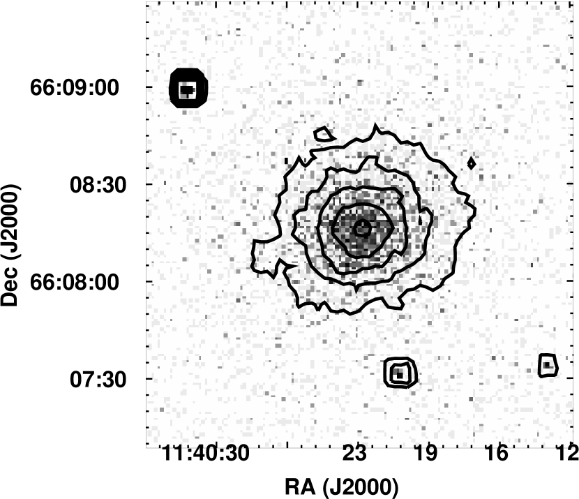
Figure 1: Raw 0.3 keV to 10.0 keV image of MS1137.5+6625, blocked into 2^′′ pixels. There are approximately 4,000 cluster counts in 107 ks of time. No background subtraction has been performed. The contours are logarithmically spaced from 0.55 to 30 counts, where the map has been smoothed over 4 pixels. The aimpoint is $\sim$ 1 arcmin south and $\sim$2.5 arcmin east of the cluster’s center; the instrument PSF is nearly unchanged from the aimpoint at the cluster’s position.

MS 1137.5+6625 was observed from September 30 to October 2, 1999 for an elapsed live time of 117.712 ks. The aimpoint of the ACIS-I3 chip was $\sim 1^{\prime}$ south and 2.5^′ east of the cluster center. We selected events with the standard ASCA grades and rejected data taken during times with background rates more than 20% greater than the mean. The effective exposure time after this filtering was 107.045 ks. In Figure 1, we present a raw image, without a background subtracted, in the 0.3 to 10.0 keV energy range, blocked into 2^′′ pixels. There are about 4000 cluster photons in the image. The background rate in the map is about 0.15 counts arcsec^-2; the average emission rate over the cluster area is about four times brighter. In the image, the cluster looks relaxed and symmetric.

3.1 Temperature Structure

To determine the cluster’s emission-weighted temperature, we extract the cluster spectrum within 63^′′ (506 $h_{65}^{-1}$ kpc) from the cluster’s center. We estimate the background in the same region using a number of long integrations on blank fields compiled by Markevitch. (See http://hea-www.harvard.edu/$\sim$maxim/axaf/acisbg/ for a complete description of the background datasets and their reduction.) We use the background data set taken coevally with the MS 1137.5+6625 observations, so that the Chandra focal plane was at the same temperature ($-$110 C). We use Vikhlinin’s calcrmf package to derive response matrices and effective area files for the cluster spectrum; this software ensures that the variation of the energy response across the I3 chip is taken into account. Before extracting the spectra, we mask out the pointlike sources in the observed field. This has little effect on the number of cluster photons we can retrieve; only one source, $\sim$45^′′ southwest of the cluster center, was within the cluster spectrum extraction region. The spectrum contains $\sim$4200 cluster photons and $\sim$1800 background photons.

We fit this spectrum, grouped into channels with a minimum of 20 counts to ensure applicability of the $\chi^{2}$ fit statistic, to a single-temperature MEKAL plasma model in the 0.7-7.5 keV energy range, using XSPEC. The lower energy bound is chosen so that we keep only the best-calibrated data. We make our best estimate of the background spectrum by an iterative process of varying the background spectrum normalization and noting how this affects the $\chi^{2}$ fit statistic for the best-fit model. Since the hard and soft components of the X-ray background originate in different physical processes (cosmic X-rays dominate the background at energies below $\sim$5 keV and cosmic rays dominate above $\sim$5 keV), the background in the MS 1137.5+6625 observation may depart from the blank-sky background differently at low and high energies. To mitigate these effects while keeping the high-energy cluster photons, we choose an upper bound of 7.5 keV for our fit. We find the best estimate of the background to be 4.5% higher than the blank-sky background file for our epoch.

We find the best-fit emission-weighted mean temperature for the intra-cluster medium to be 6.64${}^{+1.67}_{-1.20}$ at 90% confidence. The best-fit metal abundance is 0.26${}^{+0.21}_{-0.21}$ times the solar abundance as determined by Anders & Grevesse (1989), again at 90% confidence. The cluster spectrum, its best-fit model, and the fit residuals are shown in Figure 2 along with the two-parameter confidence regions for temperature and metal abundance. The neutral hydrogen column density is not strongly constrained by the data in this energy range. The 90% confidence interval is $n_{H}=2.28^{+3.76}_{-2.28}\times 10^{20}$cm^-2, consistent with the Galactic value for this direction: 1.14$\times 10^{20}$cm^-2 (Dickey & Lockman 1990). The reduced $\chi^{2}$ statistic for this fit is 1.051 for 150 degrees of freedom.

Since the density profile suggests that the gas in the cluster center may be dense enough to cool (as discussed in Section 4), we also fit the cluster’s spectrum to a MEKAL plasma plus a MEKAL cooling flow component. We fix the lower cutoff temperature to 0.2 keV and tie the upper temperature of the cooling flow to the MEKAL plasma temperature. The best fit cooling flow upper temperature is consistent with the emission-weighted temperature we found above, the cooling flow mass deposition rate is consistent with zero, and the reduced $\chi^{2}$ is not improved. We conclude that there is no spectral evidence for a cooling flow component in the cluster.

We compare these results to those obtained by Donahue et al. (1998, 1999), who found kT_e = $5.7^{+2.1}_{-1.1}$ keV and an iron abundance of $0.43^{+0.40}_{-0.37}$ times solar abundance, at 90% confidence. These results are consistent with the Chandra results. Some difference may be expected, as there are a number of bright point sources in this field which can be distinguished by Chandra and their emission removed from the cluster spectrum, but which would likely contaminate the ASCA cluster spectrum. The point sources in the I3 chip have a background-subtracted sum of about 3800 counts in the 0.7-10.0 keV band. The brightest of these pointlike sources, located $\sim$ 60^′′ to the northeast of the cluster center, contributes $\sim$ 1000 of the 3800 counts. This emphasizes the importance of good angular resolution for studies of high-redshift clusters; it is difficult to determine accurately the ICM temperature and luminosity of high-redshift clusters without the ability to exclude point sources.

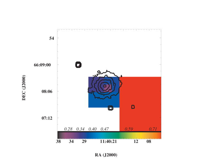
Figure 3: Hardness-ratio map of MS1137.5+6625. The cluster image in the 2.5-5.0 keV energy range is divided by the 0.5-2.5 keV image. The background is subtracted from each image and the fractional error is a constant value of 0.15 across the map. An emission-weighted temperature and abundance of 7.0 keV and 0.245 solar would give a hardness ratio of $\sim$ 0.165. Lower values correspond to lower temperatures and/or metallicity. The surface-brightness contours from Figure 1 are overlaid.

To investigate the presence of structure in the temperature or metallicity distribution in this cluster, we make a hardness ratio map using the adaptive binning technique described in Sanders & Fabian (2001). This technique ensures a constant signal-to-noise ratio across the map; we set the fractional error in each bin to be 0.10. We estimate the background in each band from the MS 1137.5+6625 dataset. In Figure 3 we show a map of the cluster in the 2.0-5.0 keV band divided by the 0.43-2.0 keV band with the surface brightness contours of Figure 1 overlaid. This ratio is sensitive to temperature variations, moderately sensitive to metal abundance variations, and essentially insensitive to neutral hydrogen absorption variations. There appear to be significant fluctuations, with the center of the cluster softer than the outer regions. The hardness ratio image appears more complicated than the raw image, suggesting variations in temperature and/or abundance may not be present in the ICM density. Such behavior is not uncommon in clusters at low redshifts. Donnelly et al. (2002) derive temperature maps for a complete sample of nearby clusters observed with the ASCA facility. Many of these clusters which appear regular in surface brightness, even in images with much better photon statistics, exhibit quite complicated temperature structure, suggesting that temperature and abundance variations, likely created during cluster merging, are either created frequently or persist for a long time.

We can quantify the structure in this map further by identifying the hardness ratios with those expected from a MEKAL plasma. A MEKAL plasma at our best-fit emission-weighted temperature of 6.7 keV and metallicity of 0.25 solar gives a hardness ratio of $\sim$0.28 in these bands. For a hardness ratio of 0.35, a $\sim$ 7 keV plasma must have an abundance of $\sim$ 1.0; or, if the abundance is to be 0.25, the plasma must be at a temperature of $\sim$10 keV.

We attempt to confirm this temperature variation by fitting spectra extracted from different regions. The first is the region within 17^′′ and the second is the annulus between 17^′′ and 47.5^′′. The best fit temperature and abundance for the inner region are 6.9${}^{+2.2}_{-1.5}$ keV and 0.21${}^{+0.26}_{-0.21}$ times solar, at 90% confidence. The best fit temperature and abundance for the outer region are 8.8${}^{+3.5}_{-2.6}$ keV and 0.28${}^{+0.39}_{-0.28}$ times solar. The data are consistent with a cooler inner region, but this is not statistically significant at 90% confidence. There are not enough photons to support a temperature deprojection analysis.

3.2 Density Profile

We parameterize the spatial distribution of the electron number density $n_{e}$ as a spherically-symmetric isothermal beta-model(cf. Cavaliere & Fusco-Femiano 1976, 1978). The beta-model has the form:

$$n_{e}(r)=n_{e0}\left(1+\frac{r^{2}}{r_{c}^{2}}\right)^{-3\beta/2},$$ (1)

where $n_{e0}$ is the electron number density at the cluster’s center; $\beta$, though derived with a physical meaning, is in practice a fitted parameter; $r_{c}$ is a characteristic length scale for the cluster, also a fitted parameter; and $r$ is the radius from the center. Thermal bremsstrahlung X-ray emission from such a plasma results in a surface brightness profile of the form

$$S_{X}(\theta)=S_{X0}\left(1+\frac{\theta^{2}}{\theta_{c}^{2}}\right)^{\frac{1}{2}-3\beta},$$ (2)

where $S_{X0}$ is the surface brightness at the center of the cluster, $\theta_{c}$ is the cluster’s projected core radius $\theta_{c}={{\rm r}_{c}/D_{A}}$, and $\theta$ is the angular distance from the cluster center. Using the CXC Sherpa package, we fit an image made in the energy range 0.3 keV to 5.0 keV to a generalized beta-model, in which two perpendicular axes can have different core radii. (As noted by Fabricant et al. (1984), a biaxial ellipsoid with a beta-model electron-density distribution will project to a simple elliptical beta-model of this type for any orientation of the axes with respect to the observer.) The axis ratio, i.e., the ratio of the minor to the major axis, is 0.87${}^{+0.06}_{-0.07}$, at 90% confidence. We use the image analysis to quantify the deviation from circular symmetry and to locate the cluster’s center. However, using a biaxial or triaxial cluster model introduces a considerable amount of ambiguity, cf. Grego et al. (2000). We use a spherically symmetric model, checking that the best-fit shape parameters from the two-dimensional fit are consistent with those from the spherically symmetric model, and leave the discussion of the effects of deviations from spherical symmetry until Section 6.

Using the centroid from the two-dimensional fit (RA = 11^h40^m22^′′.4, Dec.= +66^∘ 08^′ 14^′′.7), we derive a one-dimensional surface brightness profile and fit it to the beta-model of Equation 2. We model the background (as a constant) concurrently with the cluster model, so that we can use the log-likelihood statistic (called the “Cash” statistic in Sherpa). This statistic, $S\equiv-2ln(L)$ where $L$ is the Poisson likelihood, tends asymptotically to be distributed like the $\chi^{2}$ statistic, so confidence intervals on the calculated quantity can be constructed by the deviation from the minimum statistic. Over the small angular region within which we are fitting (within a radius of 85^′′) and in this energy band, the effective area of Chandra changes by less than 3% and the background (as estimated from the Markevitch background files) is constant. We also allow for an offset between the centroid we determined from the image analysis and the surface brightness peak. In Figure 4 we show the data, the best fit model, and the fit residuals; the best-fit model has $\beta$=0.63 and a core radius of 13.3^′′, or 106 $h_{65}^{-1}$ kpc. The confidence intervals on the surface-brightness shape parameters are shown in the right panel of the figure. For the confidence interval calculation, the offset between the centroid and peak is fixed to its best-fit value of $2.1^{\prime\prime}$, reasonable for a cluster with the observed axis ratio. If we require the peak to coincide with the centroid, the best-fit core-radius decreases to 10.9^′′, the best-fit $\beta$ is 0.56, and the fit statistic degrades by $\Delta S$=1.6. The small core radius of this cluster reinforces the importance of Chandra’s high angular resoution for studying high-redshift clusters.

We fit this profile again, after eliminating the central region, to see if the small (and marginally statistically significant) central excess is affecting the shape parameter fit, and we find no appreciable change in the fitted parameters.

We recover the central gas density from the normalization of the fitted XSPEC model to the spectrum. The XSPEC normalization is as follows:

$$N_{XS}={10^{-14}\over 4\pi(1+z)^{2}D_{A}^{2}}\int n_{H}n_{e}dV,$$ (3)

where the integral is taken over the volume projected onto the area within which the spectrum was extracted, here, within a circular region with radius R. All variables are in cgs units. The central density can be found from this relation:

$$n_{e0}^{2} = {4\,\pi\,(1+z)^{2}D_{A}\,^{2}N_{XS}\over 10^{-14}\,(n_{H}/n_{e})}\left({1-3\beta\over 2\,\pi r_{c}^{3}}\right)$$ (4)

$$\times \left[\int\limits_{0}^{\infty}\left\{\left(1+\zeta^{2}+{R^{2}\over r_{c}^{2}}\right)^{1-3\beta}-\left(1+\zeta^{2}\right)^{1-3\beta}\right\}d\zeta\right]^{-1},$$

where $\zeta$ is the distance from the cluster center along the line of sight in units of the core radius.

To determine the uncertainty in the central electron density measurement due to the spatial fits, we calculate n_e0 at a large number of parameter pairs (grid points) distributed over the 90% confidence interval on $\theta_{c}$, $\beta$ of Figure 4b. Determining the confidence interval on $n_{e0}$ from the relevant confidence area for $\theta_{c}$ and $\beta$ is necessary to correctly account for the strong correlation between parameters. We add in quadrature the spectrum normalization uncertainty and the uncertainty from the spatial fits. We find a central density of 0.0136${}^{+0.0016}_{-0.0013}$ cm^-3. In Figure 5, we illustrate the relative contributions of the uncertainties; we plot with a solid line the $n_{e}(r)$ calculated for each grid point within the 90% confidence interval (the contribution from the spatial fit) and with a dashed line the 90% confidence interval on $n_{e}(r)$ which includes the contribution from the uncertainty in the XSPEC normalization. We note that uncertainty is dominated by the uncertainty in the shape parameters.

4 Calculated Quantities

4.1 Cooling Profile

We calculate the cooling time of the ICM as a function of cluster radius, using the ratio $(5kT_{e}/2)/(\epsilon_{ff}(T_{e})n_{e}(r))$, where $\epsilon_{ff}(T_{e})$ is the free-free emissivity of a plasma with our best-fit abundance (line emission contributes very little cooling at 7 keV). The cooling time in Gyr as a function of cluster radius is shown in the left panel of Figure 6. In the right panel, we compare the cooling time to the age of the universe at the cluster’s epoch, which is 7.53 $h_{65}^{-1}$ Gyr in our chosen cosmology. The cooling time of the ICM appears to be shorter than the cluster’s age at radii below 25-70 $h_{65}^{-1}$ kpc. However, we do not see convincing evidence for a cooling flow in the cluster’s image or spectrum. For the cooling time in the center of the cluster to be longer than the cluster’s age, one or more of our assumptions must be incorrect. There could be a source of heat to the gas at the cluster center (although there is no evidence for a radio-loud galaxy there). The cosmology we use could be incorrect, but for the cooling time to be longer than the cluster’s age with certainty, $h$ must be greater than 1.0 for an $\Omega_{M}$=0.3 flat universe, or $\Omega_{M}$=0.8 if $h$ is $\sim$ 0.65 in a flat universe. It is also possible that our simplified physical model for the cluster is incorrect; if the gravitational potential is steeper along the line of sight than it appears in projection, the central density we calculate would be overestimated, and the cooling time underestimated. A relatively modest change of $\theta_{c}$(line of sight)/$\theta_{c}$(projected) = 0.8 can lower the central density by $\sim$50%. Or the cluster may have formed or undergone a merger with enough power to disrupt cooling processes at some time more recent than $t_{cool}$.

4.2 Gas and Total Mass Profiles

The gas mass profile follows directly from the electron number density profile (cf. Sarazin 1988):

$$M_{g}(R)=4\pi\int\limits_{0}^{R}n_{e}(r)\,\mu_{e}m_{p}\,r^{2}\,dr.$$ (5)

We use the best-fit abundance to calculate the mean atomic mass $\mu m_{p}$ and assume $\mu$ is constant throughout the gas, and that the plasma is fully ionized. We calculate the cluster’s total mass under the assumption that the ICM is isothermal and in hydrostatic equilibrium in the cluster potential, with thermal support only. Under such assumptions, the total mass of a cluster within radius $R$ is

$$M(R)={3kT_{e}\beta\over G\mu m_{p}}{R^{3}\over r_{c}^{2}+R^{2}},$$ (6)

where G is the gravitational constant.

The resulting gas mass fraction profile is shown in Figure 5, where again we use solid lines to trace $f_{g}(r)$ for the allowed shape parameters and the dashed lines to delineate the 90% confidence interval which includes the uncertainties in $N_{XS}$ and $T_{e}$. We compare the left and right panels of Figure 5 and note that the statistical uncertainty is dominated by the uncertainty in $T_{e}$.

We compare the gas mass fraction we calculate with the Chandra data with the gas mass fraction determined using Sunyaev-Zel’dovich effect data. We use the method described in Grego et al. (2001) which was used to determine the gas mass fraction from interferometric SZE data and published ASCA temperatures. The method uses the SZE data to constrain the cluster’s shape parameters $\beta$ and $\theta_{c}$ and X-ray spectra to determine the emission-weighted temperature, which is combined with the SZE normalization and shape parameters to determine $n_{e0}$. To better compare the masses, we rederive the SZE $f_{g}$ using the Chandra temperature from Section 3.1. The SZE/Chandra-determined gas mass within 63^′′ is $3.0^{+0.7}_{-1.0}\times 10^{13}h_{65}^{-2}$ M_⊙ and the gas mass fraction within 63^′′ is $0.06^{+0.07}_{-0.03}h^{-1}_{65}$. The precision of the temperature measurement is greatly improved from that used in Grego et al. (2001); this is masked somewhat by our choice here to use the 90% confidence interval rather than the 68% confidence interval. We compare these to the gas mass and gas mass fraction determined in this work from the Chandra data alone: a gas mass of 2.1${}^{+0.1}_{-0.1}\times 10^{13}h_{65}^{-5/2}$ M_⊙ and a gas mass fraction of 0.157${}^{+0.022}_{-0.044}h_{65}^{-3/2}$. The results are summarized in Table 1. The gas mass and gas mass fraction measurements are marginally consistent at 90% confidence.

To compare the total mass estimate with the weak lensing measurement, we calculate the total cluster mass projected within a radius of 2^′. We integrate the mass density along the line of sight to $\sim$20 core radii, or about 1.5 Mpc; if we integrate out twice as far, the total mass changes by only $\sim$15%. The projected cluster mass within 2^′ determined from the Chandra data is 6.0${}^{+1.7}_{-1.2}\times$10¹⁴M${}_{\odot}h_{65}^{-1}$. This is quite consistent with the minimum projected mass of $(4.9\pm 1.6)\times 10^{14}h_{65}^{-1}M_{\odot}$ calculated from the Clowe et al. (2000) weak lensing estimate.

We note here that the cluster’s lensing-derived mass profile appears more compact than expected. In their weak lensing analysis, Clowe et al. (2000) compare the calculated mass profile to the Navarro et al. (1996) universal profile and find MS 1137.5+6625 is more centrally concentrated than is usual for massive clusters in this scenario. (The Navarro et al. (1996) profile has since been noticed to generally predict steeper density distributions than observed, so this is particularly striking.) MS 1137.5+6625 also exhibits a number of lensed arcs in the cluster center, again indicating a high central mass concentration. Clowe et al. (2000) find these points suggestive, but not conclusive, of an elongation of the cluster along the line of sight. Our analysis of this cluster shows a core radius of $\sim$ 100 ${}_{65}^{-1}$ kpc. This is certainly more compact than the bulk of nearby clusters, whose core radii are generally around 150 $h_{65}^{-1}$ kpc (Jones & Forman 1999; Mohr et al. 1995). Only 11 of the 45 clusters in the Mohr et al. (1995) sample have core radii as small or smaller than this, yet the temperature of MS 1137.5+6625 has a higher emission-weighted temperature, and is therefore presumably more massive, than 28 of the clusters in the sample. The cluster may then fall into the compact-core radius group of Ota & Mitsuda (2002), which divides clusters into two distinct groups, one with core radii around 60 kpc, and one with core radii 220 kpc. Although a full investigation into correlations between core radius size and other properties has yet to be done, Ota & Mitsuda (2002) find evidence that clusters with cD galaxies have small core radii and that the luminosity-temperature relationships for the two cluster populations have different normalizations, though similar slopes.

5 Cluster Distance

We derive the cluster’s angular diameter distance by comparing the cluster’s X-ray emission and Sunyaev-Zel’dovich Effect (SZE) data. The method closely follows the method used in Reese et al. (2000), except that in this work we use Chandra imaging and spectral data instead of ROSAT imaging and ASCA spectral data.

The SZE has a magnitude proportional to the Compton $y$-parameter, i.e., the total number of scatterers, weighted by their associated temperature,

$$y={{k\sigma_{T}}\over{m_{e}c^{2}}}\int{n_{e}(l)T_{e}(l)dl},$$ (7)

where $k$ is Boltzmann’s constant, $\sigma_{T}$ is the Thomson scattering cross section, $m_{e}$ is the electron mass. For an isothermal beta-model, the projected SZE effect would be:

$$\Delta T=f_{(x,T_{e})}T_{CMB}D_{A}\!\int\!\!d\zeta\,\sigma_{T}n_{e}\frac{k_{B}T_{e}}{m_{e}c^{2}}=\Delta T_{0}\left(1+\frac{\theta^{2}}{\theta_{c}^{2}}\right)^{(1-3\beta)/2},$$ (8)

where $\Delta T$ is the thermodynamic SZE temperature decrement/increment and $f_{(x,T_{e})}$ is the frequency dependence of the SZE, with $x=h\nu/kT_{CMB}$, where $T_{CMB}$ is the temperature of the cosmic microwave radiation $T_{CMB}$=2.728 (Fixsen et al. 1996). In the non-relativistic and Rayleigh-Jeans limits, $f_{(x,T_{e})}\sim-2$; we apply the relativistic corrections of Itoh et al. (1998) to fifth order in $kT_{e}/m_{e}c^{2}$, so that $f_{(x,T_{e})}=-1.907$.

Extending Equation 2, the cluster’s projected X-ray surface brightness is

$$S_{X}=\frac{1}{4\pi(1+z)^{4}}D_{A}\!\int\!\!d\zeta\,n_{e}n_{H}\Lambda_{eH}\>\;\!=S_{X0}\left(1+\frac{\theta^{2}}{\theta_{c}^{2}}\right)^{\frac{1}{2}-3\beta},$$ (9)

where $S_{X}$ is the X-ray surface brightness in erg s^-1 cm^-2 arcmin^-2, $z$ is the cluster’s redshift, n_H is the hydrogen number density of the ICM, $\Lambda_{eH}=\Lambda_{eH}(T_{e},\mbox{abundance})$ is the X-ray cooling function of the ICM in the cluster rest frame in erg cm³ s^-1 integrated over the redshifted Chandra band, and $S_{X0}$ is the X-ray surface brightness at the center of the cluster. We convert the X-ray detector counts to cgs units using the Chandra response matrices available from http://asc.harvard.edu/cal/Links/Acis/acis/; the conversion factor is 7.91$\times 10^{-12}$ erg cm^-2 s^-1. One can solve for the angular diameter distance by eliminating $n_{e0}$.

We perform a joint fit to the interferometric SZE data and the Chandra image, in which the X-ray pointlike sources have been masked out. We compare the X-ray data to a beta model with a constant cosmic background; this model is exposure-corrected before the fit. The logarithm of the Poisson likelihood is then calculated. The interferometric SZE observations provide constraints in the Fourier ($u$-$v$) plane, so we perform our model fitting in the $u$-$v$ plane, where the noise properties of the data and the spatial filtering of the interferometer are well defined. The Gaussian likelihood is calculated using the SZE model and the SZE data. There are no detected point sources in the SZE data. We use a downhill simplex method (Press et al. 1992) to search the parameter space and maximize the joint likelihood of the cluster position, $\beta$, $\theta_{c}$, $S_{X0}$, $\Delta To$, and cosmic X-ray background.

Each data set is independent, and likelihoods from each data set can simply be multiplied together to construct the joint likelihood. From this we can generate confidence regions for the parameters.

Uncertainties in the angular diameter distance from the fit parameters are calculated by gridding (stepping) in the interesting parameters to explore the $\Delta S$ likelihood space. As a compromise between precision and computation time, we grid in $\Delta T_{0}$, $S_{X0}$, $\beta$, and $\theta_{c}$ allowing the X-ray background to float while fixing the positions of the cluster (both SZE and X-ray). From this four dimensional $\Delta S$ hyper-surface, we construct the 90% confidence interval for $D_{A}$ due to $S_{X0}$, $\Delta T_{0}$, $\beta$, and $\theta_{c}$ jointly. The correlations between the beta-model parameters require this treatment to determine accurately the uncertainty in $D_{A}$ from the fitted parameters. We emphasize that these uncertainties are meaningful only within the context of the spherical isothermal $\beta$ model.

In the Reese et al. (2002) work, the calculated angular diameter distance of MS 1137.5+6625 using ROSAT and ASCA data was 3179${}^{+1103}_{-1640}h^{-1}$ Mpc (statistical uncertainty only), at 68% confidence. In our analysis here, with a more accurate emission-weighted temperature and improved X-ray imaging data, we find an angular diameter distance (at 90% confidence) of 3439${}^{+1854}_{-2087}h^{-1}$ Mpc, which implies a Hubble constant of 31${}^{+19}_{-17}$ km s^-1 Mpc^-1 (with statistical uncertainties only). The Chandra observation moderately improves the precision of the measurement, but do not rectify it with the Reese et al. (2002) sample; the derived Hubble constant is still $\sim 2.5\sigma$ from the 18 cluster sample average.. MS 1137.5+6625 is a peculiar cluster, and in the next section we discuss our calculations and attempt to discern how this cluster may deviate from a relaxed, spherical, isothermal cluster.

6 Discussion

The X-ray and optical images of the distant galaxy cluster MS1137.5+6625 show the X-ray surface brightness and optical light have a regular, symmetric, and quite compact distribution. However, several lines of evidence suggest that the cluster structure is more complicated:

• The hardness ratio map and spectral analysis suggest that the cluster has a relatively more complicated temperature and metal abundance structure than density structure.

• The gas mass fraction calculated from the SZE/Chandra data is only marginally consistent with the gas mass fraction calculated from the X-ray data.

• The Hubble constant calculated for this cluster is low by a factor of $\sim$2. (This is closely related to the discrepancy in the gas mass fraction and gas mass.)

These calculated quantities are summarized in Table 1. The most compelling argument that MS 1137.5+6625 deviates from isothermal, spherical symmetry is that the Hubble constant value derived from it is so low. The X-ray and SZE data sets are not sensitive enough individually to allow us to definitively test our assumptions, but taken together they do provide some insight. Here, we discuss a number of possible explanations for our observations.

6.1 SZE Data Systematics

The possible contribution to systematic uncertainty to the Hubble constant and gas mass fraction measurement by the SZE data itself is very low. It is possible that there are undetected radio-bright point sources in the cluster field. Unless they are unfortunately placed on the sidelobes, point sources will decrease the measured SZE effect and increase the measured $H_{\circ}$. Combining the SZE observations with 1.4 GHz NVSS (Condon et al. 1998) observations suggests that possible undetected point sources in the MS 1137.5+6625 field have a negligible effect on the derived Hubble parameter (Reese et al. 2002). We find no evidence for a radio halo in this cluster in the NVSS image. Radio haloes, i.e., large scale diffuse radio emission, would again depress the measured SZE and therefore would cause an overestimate of the Hubble constant.

Anisotropies of the CMB of other types which might affect the SZE data are at very low levels. A limit to the primary anisotropies at these angular scales was set by Dawson et al. (2001) and Holzapfel et al. (2000). They find the Rayleigh-Jeans temperature of these fluctuations to be less than 14 $\mu$K, and this in turn should contribute less than 2% uncertainty to $H_{\circ}$. Confusion from the kinematic SZE effect (the spectral distortion of the CMB made by the cluster moving with respect to the CMB rest frame) should also be quite small; for an 8 keV cluster moving with a 300 km s^-1 velocity component in the line of sight direction, the kinetic SZE effect will be $\sim$4% of the thermal SZE (and the sign of the effect will depend on whether the cluster is moving towards or away from the observer) leading to an 8% error in the Hubble constant. It is therefore quite unlikely for the SZE to be severely in error due to peculiar velocity of the cluster gas.

6.2 Geometry

The Hubble constant is derived under the assumption that the cluster can be characterized by a spherically symmetric distribution. This will be in error by the ratio of the projected cluster size $L_{PROJ}$ to the line of sight cluster size $L_{LOS}$: $H_{meas}=H_{true}\times\,L_{PROJ}/L_{LOS}$. We have measured the apparent axis ratio to be 0.87${}^{+0.06}_{-0.07}$ for the elliptical beta model; the core radius measured by the circular beta model is roughly the geometric mean of the two axes. For an apparently circular distribution, the line of sight axis could be longer or shorter than the projected axis, leading to a prolate or oblate three dimensional cluster, respectively. For an apparently elliptical mass distribution, the true three-dimensional distribution has another degree of complexity in addition to the degree of prolateness or oblateness; the axis of symmetry could have any angle of inclination with respect to the plane of the sky, allowing the symmetry axis an essentially infinite range of lengths which would produce the same projected image. Additionally, there is no a priori reason that clusters need to be ellipsoidally symmetric; in fact, for axis ratios of less than $1/\sqrt{2}$, the concentrically ellipsoidal isothermal beta-model for the density distribution is unphysical (cf. Grego et al. 2000) if the the cluster is indeed in hydrostatic equilibrium. The gravitational potential supporting such a beta-model requires negative dark matter density. A more sophisticated model for the non-spherical density distribution is clearly required in such cases, but is beyond the scope of this paper. We note that for measuring cosmological parameters from an ensemble of clusters, increasing the complexity of the model is not strictly necessary. For example, (Sulkanen 1999) shows that from a sample of triaxial clusters, one can reconstruct an unbiased estimator for the Hubble constant by using a spherical model.

In the simplest picture, the error in the Hubble constant is approximately the ratio of the apparent cluster size (i.e., the geometric mean of the two core radii) to the line of sight size. In such a picture, for MS 1137.5+6625’s measured Hubble constant to equal the sample mean of Reese et al. (2002), L(projected)/L(line of sight) must be 0.58. As a fiducial point, in a flux limited sample of clusters fitted with elliptical beta-models, Mohr et al. (1995) measure an axis ratio for the sample of 0.8${}^{+0.14}_{-0.11}$. For the low Hubble constant to be due solely to an elongated cluster, it would have to be have two unusual characteristics for a cluster chosen from an unbiased sample: it would have a much longer axis ratio than generally observed in projection, and would have its symmetry axis nearly aligned with the line of sight, basically a long cigar pointed at the observer. If the symmetry axis were not nearly along the line of sight, the true axis ratio would need to be even greater.

Since such an elongation along the line of sight is so unexpected, this may indicate that the criteria by which MS 1137.5+6625 was detected favored such clusters. MS 1137.5+6625 was originally identified in the EMSS (Gioia et al. 1990), using a 2.${}^{\prime}4\times 2.^{\prime}4$ detection cell, a size which would just fit the cluster emission we observe with Chandra. It was detected with a signal-to-noise ratio of 5.3 in a survey with minimum S/N for detection of 4.0. MS 1137.5+6625 is the coolest and least luminous of the z $>$ 0.5 clusters in the EMSS survey. If there does exist a population of similarly luminous, highly elongated clusters at high redshifts, it is likely that only those aligned very nearly along the line of sight would be detected by this survey; a cluster also near the detection cutoff but which was elongated in the plane of the sky would deposit less of its flux into a single detection cell and may not be detected. For example, if MS 1137.5+6625 had an intrinsic axis ratio of $\sim$0.75 but with the major axis in the plane of the sky, it is unlikely that it would have been detected with sufficient significance to be included in the survey.

The selection effects from the original point-source algorithm used for the EMSS were discussed in Pesce et al. (1990), and reprocessing of the Einstein data led Lewis et al. (2002) to conclude that the EMSS survey systematically missed clusters of low surface brightness. Similarly, simulations of the EMSS detection algorithm by Ebeling et al. (2000) suggest the algorithm may miss clusters with significant substructure.

6.3 Temperature Gradients

Although we have no compelling evidence for a cooling flow at the cluster’s center, we do have evidence of structure in the temperature and abundance distribution. Temperature structure could affect both the derived shape parameters and the derived emission-weighted temperature.

Temperature structure will affect the X-ray and SZE data differently. It should not strongly affect the X-ray-derived spatial shape parameters; for a given emission measure, the emitted flux in the band we use for spatial fitting only changes by $\sim$ 20% for gas with kT_e from 4 keV to 10 keV. Also, for the X-ray spatial fitting, the data are azimuthally averaged, so that such structure would have little effect.

The SZE measurements, by virtue of the spatial filtering inherent in interferometry, are insensitive to temperature gradients on scales larger than a few arcminutes, but can be quite sensitive to smaller scale gradients. As the SZE effect is proportional to $n_{e}\times T_{e}$, the density inferred at any particular point will be over (under) estimated from an under (over) estimate of the temperature. Temperature structure could result in the beta-model fitted to the SZE differing from that fitted to the X-ray data. We do not expect this poor fit to the beta-model to strongly affect the calculated Hubble constant, because the joint-fit to the model is dominated by the X-ray imaging data in this case. It may, however, affect strongly the gas mass fraction determined from the SZE data, as this is derived from the SZE spatial fits.

If MS 1137.5+6625 had a non-hydrostatic pressure structure, then we may expect to see evidence of this in the SZE data. The low surface brightness of the SZE-effect makes it difficult to image on small scales, however, and with the current data, we are unable to make a conclusion about non-hydrostatic pressure. Future generations of SZE instruments may have such capability.

The temperature structure of the cluster could contribute to the low value of the Hubble constant in another way. The temperature we use for the $H_{\circ}$ calculation is the emission-weighted temperature, and the relevant quantity for the calculation is actually the density-weighted temperature. As a fiducial point for the discussion, we compare the emission-weighted temperature and the density-weighted temperature for a cluster with the following structure: $\beta$ equal to the best-fit value from our model fit, and gas within two core radii ($\sim$200 kpc) at half the temperature of the gas from two core radii to ten: $T_{e}(r<2r_{c})=0.5\times T_{e}(2r_{c}<r<10r_{c})$. Temperature structure of this magnitude, while unusually pronounced, has been observed by Chandra in the cluster Abell 1835 (Schmidt et al. 2001), a massive cooling-flow cluster with highly luminous optical emission-line nebulae. In such a scheme, the emission-weighted temperature would be 0.80 times the density-weighted temperature, and the Hubble constant would be 0.64 times the true Hubble constant. For the underestimation of the Hubble constant to be due solely to an underestimate of the temperature, the emission-weighted temperature must be $\sim$0.65-0.70 times the density-weighted temperature. We stress that this is a simple calculation; the exact effect depends also on the specifics of the instruments used to make the measurements. However, even if MS 1137.5+6625 had as extreme a temperature gradient as the atypical Abell 1835, this could not explain the entire Hubble constant underestimate.

7 Summary

In conclusion, the massive, distant galaxy cluster MS 1137.5+6625 appears compact and regular in its optical and X-ray images, but evidence suggests that it is not an isothermal, spherical cluster. The Hubble constant calculated for the cluster from X-ray imaging and spectra and interferometric SZE data is unusually low.

Many of the known systematic effects in the X-ray/SZE Hubble constant measurement tend to make the Hubble constant higher, and few effects make it lower. (A thorough discussion of these systematic effects can be found in Reese et al. (2002).) Two effects which can make the measured Hubble constant artificially low are elongation along the line of sight and temperature structure in the ICM. We have evidence suggestive of a line of sight elongation. The optical lensing data indicate the surface mass density is quite high, as evidenced by strongly lensed arcs, and that the mass distribution is very compact. The X-ray data show the ICM density distribution is unusually compact, as well. We see structure in the hardness ratio map which could be interpreted as temperature structure, with cooler or less metal-enriched gas at the center of the cluster.

We also compare other calculated quantities besides the Hubble constant to investigate the systematic effects. The SZE-derived gas mass is completely insensitive to geometry, though it is quite sensitive to temperature structure; if the emission-weighted temperature were biased low, the SZE gas mass would be an overestimate of the true gas mass. The X-ray-derived gas mass is essentially insensitive to temperature structure, but has a moderate dependence on geometry; if the cluster were elongated along the line of sight, the X-ray gas mass would be a slight overestimate. The X-ray-derived gas mass is 2.1${}^{+0.1}_{-0.1}\ h_{65}^{-5/2}\times 10^{13}M_{\circ}$ and the SZE-derived mass is $3.0^{+1.0}_{-1.0}\ h_{65}^{-2}\times 10^{13}M_{\circ}$. Within the uncertainty the masses agree and we cannot place strong limits on temperature structure and elongation with the current datasets.

We conclude with two points: one, that cluster appearance is a poor criterion for choosing sources for cosmological tests. MS 1137.5+6625 appeared as a possibly ideal cluster for cosmology, with its regular, compact, round, X-ray and optical images, and no evidence of a strong cooling flow. However, it yields a Hubble constant measurement which is strikingly low. We stress that a cluster sample must be selected via well-defined, objective criteria. And two, that selection effects in the parent sample from which the clusters are drawn should be well-understood, i.e., although for cosmological work we generally select clusters from existing X-ray surveys on the basis of luminosity rather than surface brightness, any selection for surface brightness in the X-ray survey itself will still be present in the luminosity-selected sample. This situation can be ameliorated by future cluster surveys, such as the SZE survey discussed in Holder & Carlstrom (2001), which have selection functions different from the X-ray and optical cluster surveys.

8 Acknowledgements

We are very sad to note that Leon VanSpeybroeck passed away at the end of 2002. He was an excellent scientist and colleague and friend. We remain inspired by his example.

Many thanks to the referee for her insightful comments that improved this paper. We gratefully acknowledge the contributions of several people who developed public-use tools which we used extensively: Maxim Markevitch for the blank field background data sets, Alexey Vikhlinin for the X-ray data analysis software, and J. S. Sanders and A. C. Fabian for the adaptive binning software. We thank the CLEGS group at the CfA for helpful discussion. EDR acknowledges support from the NASA Chandra Postdoctoral Fellowship PF 1-20020. This work was supported in part by the NASA grants NAG5-4985, GO0-1037X, NAG5-10071, and GO1-2138X.

Table 1: Summary of Derived Properties

Data	gas mass	total mass	$f_{g}$	$D_{A}$
	$10^{13}M_{\circ}$	$10^{14}M_{\odot}$		(Mpc)
	within 63′′	projected within 120′′	within 63′′	(for $\Omega_{M}=0.3$, $\Omega_{\Lambda}=0.7$)
Chandra	2.1${}^{+0.1}_{-0.1}\ h_{65}^{-5/2}$	6.0${}^{+1.7}_{-1.2}\ h_{65}^{-1}$	0.157${}^{+0.022}_{-0.044}\ h_{65}^{-3/2}$	—
SZE	$3.0^{+1.0}_{-1.0}\ h_{65}^{-2}$	—	$0.06^{+0.07}_{-0.03}\ h^{-1}_{65}$	—
SZE/Chandra	—	—	—	3439${}^{+1854}_{-2087}h_{65}^{-1}$
Keck Weak Lensing	—	4.9${}^{+1.6}_{-1.6}\ h_{65}^{-1}$	—	—

Figure 2: Left panel: the Chandra ACIS-I spectrum, best-fit model, and residuals for the full cluster spectrum for MS 1137.5+6625. Right panel: the two-parameter confidence region for emission-weighted temperature (kT_e) and abundance. The first, third, and fourth regions correspond to 68.3%, 90%, and 99.0% confidence on the two parameters jointly. The projection of the second region onto either axis marks the 90% confidence interval on the single parameter. The ‘+’ marks the best-fit value.

Figure 4: Left panel: One-dimensional surface brightness profile of cluster MS1137.5+6625 with background, its best-fit beta-model, and fit residuals in units of the standard deviation $\sigma$.. Right panel: Two-parameter confidence region for $\beta$ and $\theta_{c}$ for the one-dimensional beta-model fit to MS1137.5+6625. The confidence contWe use values $\Omega_{M}$ = 0.3 and $\Omega_{\Lambda}$= 0.7.ours correspond to 68.3%, 90%, 93% and 99.0% confidence on the two parameters. The projection of the 93% confidence interval onto an axis gives the single-parameter 90% confidence interval. The best-fit model is marked with a ‘+’.

Figure 5: Left. Electron number density versus radius in kpc. Right. The gas mass fraction of the cluster as a function of cluster radius in kpc. The solid lines show n${}_{e}(r)$ and $f_{g}(r)$ for parameter grid points within the 90% confidence region of the fitted model. The dashed lines show the full 90% confidence intervals for n${}_{e}(r)$ and $f_{g}(r)$, which includes the uncertainty in the spectrum’s normalization for n${}_{e}(r)$, and in the spectrum’s normalization and emission-weighted $T_{e}$ for $f_{g}(r)$. The calculations are done using values $\Omega_{M}$ = 0.3 and $\Omega_{\Lambda}$= 0.7.

Figure 6: Left panel: The cooling time of the ICM in Gyr as a function of cluster radius in kpc. Right panel: The cooling time of the ICM in units of the age of the universe at the cluster’s redshift, as a function of cluster radius in kpc. The calculations are done using values $\Omega_{M}$ = 0.3 and $\Omega_{\Lambda}$= 0.7. Again, the solid lines show the cooling times calculated for the parameter grid points within the 90% confidence region of the fitted model and the dashed lines show the full 90% confidence intervals including the uncertainty in $N_{XS}$ and $T_{e}$. The age of the universe at the cluster’s epoch is 7.53 Gyr $h_{65}^{-1}$.

References

- Allen & Fabian (1998) Allen, S. W. & Fabian, A. C. 1998, MNRAS, 297, L57
- Anders & Grevesse (1989) Anders, E. & Grevesse, N. 1989, Geochim. Cosmochim. Acta, 53, 197
- Arnaud & Evrard (1999) Arnaud, M. & Evrard, A. E. 1999, MNRAS, 305, 631
- Bahcall & Cen (1992) Bahcall, N. A. & Cen, R. 1992, ApJ, 398, L81
- Bahcall & Fan (1998) Bahcall, N. A. & Fan, X. 1998, ApJ, 504, 1
- Birkinshaw & Hughes (1994) Birkinshaw, M. & Hughes, J. P. 1994, ApJ, 420, 33
- Birkinshaw et al. (1991) Birkinshaw, M., Hughes, J. P., & Arnaud, K. A. 1991, ApJ, 379, 466
- Cavaliere & Fusco-Femiano (1976) Cavaliere, A. & Fusco-Femiano, R. 1976, A&A, 49, 137
- Cavaliere & Fusco-Femiano (1978) —. 1978, A&A, 70, 677
- Clowe et al. (2000) Clowe, D., Luppino, G. A., Kaiser, N., & Gioia, I. M. 2000, ApJ, 539, 540
- Condon et al. (1998) Condon, J. J., Cotton, W. D., Greisen, E. W., Yin, Q. F., Perley, R. A., Taylor, G. B., & Broderick, J. J. 1998, AJ, 115, 1693
- David et al. (1995) David, L. P., Jones, C., & Forman, W. 1995, ApJ, 445, 578
- Dawson et al. (2001) Dawson, K. S., Holzapfel, W. L., Carlstrom, J. E., Joy, M., LaRoque, S. J., & Reese, E. D. 2001, ApJ, 553, L1
- Dickey & Lockman (1990) Dickey, J. M. & Lockman, F. J. 1990, ARA&A, 28, 215
- Donahue et al. (1998) Donahue, M., Voit, G. M., Gioia, I., Lupino, G., Hughes, J. P., & Stocke, J. T. 1998, ApJ, 502, 550
- Donahue et al. (1999) Donahue, M., Voit, G. M., Scharf, C. A., Gioia, I. M., Mullis, C. R., Hughes, J. P., & Stocke, J. T. 1999, ApJ, 527, 525
- Donnelly et al. (2002) Donnelly, R. H., Jones, C., Forman, W., Churazov, E., & Gilfanov, M. 2002, ApJ–in prep.
- Ebeling et al. (2000) Ebeling, H., Jones, L. R., Perlman, E., Scharf, C., Horner, D., Wegner, G., Malkan, M., Fairley, B. W., & Mullis, C. R. 2000, ApJ, 534, 133
- Eke et al. (1998) Eke, V. R., Cole, S., Frenk, C. S., & Patrick Henry, J. 1998, MNRAS, 298, 1145
- Evrard (1997) Evrard, A. E. 1997, MNRAS, 292, 289
- Fabricant et al. (1984) Fabricant, D., Rybicki, G., & Gorenstein, P. 1984, ApJ, 286, 186
- Fixsen et al. (1996) Fixsen, D. J., Cheng, E. S., Gales, J. M., Mather, J. C., Shafer, R. A., & Wright, E. L. 1996, ApJ, 473, 576
- Gioia & Luppino (1994) Gioia, I. M. & Luppino, G. A. 1994, ApJS, 94, 583
- Gioia et al. (1990) Gioia, I. M., Maccacaro, T., Schild, R. E., Wolter, A., Stocke, J. T., Morris, S. L., & Henry, J. P. 1990, ApJS, 72, 567
- Grainge et al. (2002) Grainge, K., Jones, M. E., Pooley, G., Saunders, R., Edge, A., Grainger, W. F., & Kneissl, R. . 2002, MNRAS, 333, 318
- Grego et al. (2000) Grego, L., Carlstrom, J. E., Joy, M. K., Reese, E. D., Holder, G. P., Patel, S., Cooray, A. R., & Holzapfel, W. L. 2000, ApJ, 539, 39
- Grego et al. (2001) Grego, L., Carlstrom, J. E., Reese, E. D., Holder, G. P., Holzapfel, W. L., Joy, M. K., Mohr, J. J., & Patel, S. 2001, ApJ, 552, 2
- Haiman et al. (2001) Haiman, Z. ., Mohr, J. J., & Holder, G. P. 2001, ApJ, 553, 545
- Henry et al. (1992) Henry, J. P., Gioia, I. M., Maccacaro, T., Morris, S. L., Stocke, J. T., & Wolter, A. 1992, ApJ, 386, 408
- Holder et al. (2001) Holder, G., Haiman, Z. ., & Mohr, J. J. 2001, ApJ, 560, L111
- Holder & Carlstrom (2001) Holder, G. P. & Carlstrom, J. E. 2001, ApJ, 558, 515
- Holzapfel et al. (2000) Holzapfel, W. L., Carlstrom, J. E., Grego, L., Holder, G., Joy, M., & Reese, E. D. 2000, ApJ, 539, 57
- Hughes & Birkinshaw (1998) Hughes, J. P. & Birkinshaw, M. 1998, ApJ, 501, 1
- Itoh et al. (1998) Itoh, N., Kohyama, Y., & Nozawa, S. 1998, ApJ, 502, 7
- Jones & Forman (1999) Jones, C. & Forman, W. 1999, ApJ, 511, 65
- Jones et al. (2003) Jones, M., Edge, A., Grainge, K., Grainger, W., Kneissl, R., Pooley, G., Saunders, R., Miyoshi, T., Yamashita, K., Tawara, Y., Furuzawa, A., Harada, A., & Hatsukade, I. 2003, MNRAS–submitted: astro-ph/0103046
- Lewis et al. (2002) Lewis, A. D., Stocke, J. T., Ellingson, E., & Gaidos, E. J. 2002, ApJ, 566, 744
- Luppino & Gioia (1995) Luppino, G. A. & Gioia, I. M. 1995, ApJ, 445, L77
- Mason et al. (2001) Mason, B. S., Myers, S. T., & Readhead, A. C. S. 2001, ApJ, 555, L11
- Mohr et al. (1995) Mohr, J. J., Evrard, A. E., Fabricant, D. G., & Geller, M. J. 1995, ApJ, 447, 8
- Mohr et al. (1999) Mohr, J. J., Mathiesen, B., & Evrard, A. E. 1999, ApJ, 517, 627
- Mohr et al. (2000) Mohr, J. J., Reese, E. D., Ellingson, E., Lewis, A. D., & Evrard, A. E. 2000, ApJ, 544, 109
- Mould et al. (2000) Mould, J. R., Huchra, J. P., Freedman, W. L., Kennicutt, R. C., J., Ferrarese, L., Ford, H. C., Gibson, B. K., Graham, J. A., Hughes, S. M. G., Illingworth, G. D., Kelson, D. D., Macri, L. M., Madore, B. F., Sakai, S., Sebo, K. M., Silbermann, N. A., & Stetson, P. B. 2000, ApJ, 529, 786
- Mushotzky & Scharf (1997) Mushotzky, R. F. & Scharf, C. A. 1997, ApJ, 482, L13
- Myers et al. (1997) Myers, S. T., Baker, J. E., Readhead, A. C. S., Leitch, E. M., & Herbig, T. 1997, ApJ, 485, 1
- Navarro et al. (1996) Navarro, J. F., Frenk, C. S., & White, S. D. M. 1996, ApJ, 462, 563
- Ota & Mitsuda (2002) Ota, N. & Mitsuda, K. 2002, ApJ, 567, L23
- Oukbir & Blanchard (1997) Oukbir, J. & Blanchard, A. 1997, A&A, 317, 1
- Patel et al. (2000) Patel, S. K., Joy, M., Carlstrom, J. E., Holder, G. P., Reese, E. D., Gomez, P. L., Hughes, J. P., Grego, L., & Holzapfel, W. L. 2000, ApJ, 541, 37
- Peebles et al. (1989) Peebles, P. J. E., Daly, R. A., & Juszkiewicz, R. 1989, ApJ, 347, 563
- Pen (1997) Pen, U. 1997, New Astronomy, 2, 309
- Pesce et al. (1990) Pesce, J. E., Fabian, A. C., Edge, A. C., & Johnstone, R. M. 1990, MNRAS, 244, 58
- Press et al. (1992) Press, W. H., Teukolsky, S. A., Vetterling, W. T., & Flannery, B. P. 1992, Numerical Recipes in C. The Art of Scientific Computing (Cambridge: Cambridge University Press, 2nd ed.)
- Reese et al. (2002) Reese, E. D., Carlstrom, J. E., Joy, M., Mohr, J. J., Grego, L., & Holzapfel, W. L. 2002, ApJ–submitted: astro-ph/0205350
- Reese et al. (2000) Reese, E. D., Mohr, J. J., Carlstrom, J. E., Joy, M., Grego, L., Holder, G. P., Holzapfel, W. L., Hughes, J. P., Patel, S. K., & Donahue, M. 2000, ApJ, 533, 38
- Riess et al. (1998) Riess, A. G., Filippenko, A. V., Challis, P., Clocchiatti, A., Diercks, A., Garnavich, P. M., Gilliland, R. L., Hogan, C. J., Jha, S., Kirshner, R. P., Leibundgut, B., Phillips, M. M., Reiss, D., Schmidt, B. P., Schommer, R. A., Smith, R. C., Spyromilio, J., Stubbs, C., Suntzeff, N. B., & Tonry, J. 1998, AJ, 116, 1009
- Rines et al. (1999) Rines, K., Forman, W., Pen, U., Jones, C., & Burg, R. 1999, ApJ, 517, 70
- Sanders & Fabian (2001) Sanders, J. S. & Fabian, A. C. 2001, MNRAS, 325, 178
- Sarazin (1988) Sarazin, C. L. 1988, X-ray emission from clusters of galaxies (Cambridge Astrophysics Series, Cambridge: Cambridge University Press, 1988)
- Sasaki (1996) Sasaki, S. 1996, PASJ, 48, L119
- Schmidt et al. (2001) Schmidt, R. W., Allen, S. W., & Fabian, A. C. 2001, MNRAS, 327, 1057
- Sulkanen (1999) Sulkanen, M. E. 1999, ApJ, 522, 59
- Sunyaev & Zel’dovich (1970) Sunyaev, R. A. & Zel’dovich, Y. B. 1970, Comments Astrophys. Space Phys., 2, 66
- Sunyaev & Zel’dovich (1972) —. 1972, Comments Astrophys. Space Phys., 4, 173
- White et al. (1993) White, S. D. M., Navarro, J. F., Evrard, A. E., & Frenk, C. S. 1993, Nature, 366, 429