Semi–Analytic Simulations of Galactic Winds: Volume Filling Factor, Ejection of Metals and Parameter Study

Abstract

We present a semi–analytic treatment of galactic winds within high resolution, large scale cosmological N–body simulations of a $\Lambda$CDM Universe. The evolution of winds is investigated by following the expansion of supernova driven superbubbles around the several hundred thousand galaxies that form in an approximately spherical region of space with diameter $52h^{-1}$ Mpc and mean density close to the mean density of the Universe. We focus our attention on the impact of winds on the diffuse intergalactic medium. Initial conditions for mass loss at the base of winds are taken from Shu, Mo & Mao (2003). Results are presented for the volume filling factor and the mass fraction of the IGM affected by winds and their dependence on the model parameters is carefully investigated. The mass loading efficiency of bubbles is a key factor to determine the evolution of winds and their global impact on the IGM: the higher the mass loading, the later the IGM is enriched with metals. Galaxies with $10^{9}<M_{\star}<10^{10}$ M_☉ are responsible for most of the metals ejected into the IGM at $z=3$, while galaxies with $M_{\star}<10^{9}$ M_☉ give a non negligible contribution only at higher redshifts, when larger galaxies have not yet assembled. We find a higher mean IGM metallicity than Ly$\alpha$ forest observations suggest and we argue that the discrepancy may be explained by the high temperatures of a large fraction of the metals in winds, which may not leave detectable imprints in absorption in the Ly$\alpha$ forest.

1 Introduction

Powerful outflows from star–forming galaxies have been detected throughout the history of the universe (Heckman, Armus & Miley 1990, Heckman et al. 2000, Adelberger et al. 2003), providing, perhaps, the mechanism to transport metals from the interstellar medium (ISM) of galaxies to the low density intergalactic medium (IGM). This could at least partially explain the widespread level of chemical enrichment observed in the spectra of quasars (Cowie et al. 1995, Schaye et al. 2000, Ellison et al. 1999, Simcoe, Sargent & Rauch 2004).

The energy necessary to power outflows on galactic scales is supplied by supernova explosions and winds from young massive stars in OB associations. Any episode of star formation may create a superbubble in the ISM and, if the rate of energy input is large enough, the superbubble can blow out of the ISM and create a wind. In local starbursts (Phillips 1993, Cecil, Bland-Hawthorn & Veilleux 2002, Walter, Weiss & Scoville 2002, Sugai, Davies & Ward 2003), winds have been observed to extend to at least 10 kpc from their host galaxies. Strickland & Stevens (2000) claim that winds can reach even larger distances, but are unobservable because of the low emissivity of the outflowing gas.

At present, it is difficult to predict which galaxies are responsible for seeding the IGM with metals or to establish the effects that supernova–driven blastwaves have on the galaxy formation process. While gravity does not influence the evolution of superbubbles in the ISM, it is crucial for determining the long term fate of winds. Since winds from dwarf galaxies form in shallower potential wells, they are the most likely to be able to disperse their metal content into the IGM. On the other hand, Strickland & Stevens (2000) suggest that most of the energy from winds resides in a hot ($T\sim 10^{7}$ K) low density component that can escape the galaxies even when the bulk of the outflowing mass is retained. Mac Low & Ferrara (1999) demonstrate that metals are easily accelerated to velocities larger than the escape velocity, implying that a galaxy can lose a high fraction of its metals even with a relatively low mass ejection efficiency. Although winds may occur more frequently in dwarf galaxies, the metals ejected by massive galaxies may dominate the total budget. It is therefore not a trivial problem to assess which galaxies have been responsible for the pollution of the IGM and when the enrichment occurred.

Several groups have applied simple phenomenological prescriptions to simulations in order to investigate the effects of winds on the IGM and some important results have emerged. For example, Madau, Ferrara & Rees (1999) find that pregalactic outflows are an efficient mechanism for distributing the metals produced in stars over large cosmological volumes, prior to the reionisation epoch. Aguirre et al. (2001) argue that radiation pressure ejection or winds from relatively large galaxies at lower redshifts can account for the observed metallicity of the IGM and the intracluster medium. Theuns, Mo & Schaye (2001) and Croft et al. (2002) demonstrate that cavities evacuated by winds in the outskirts of galaxies may leave characteristic signatures in the Ly$\alpha$ forest. In contrast, Theuns et al. (2002) find that winds have little effect on the statistics of H I absorption lines and produce C IV absorption lines in reasonable agreement with observations.

The significance of galactic winds for the evolution of the IGM is still not fully established, however. Both hydrodynamic and semi–analytic simulations use phenomenological prescriptions for the physics of galactic winds and new parameters have to be introduced to account for the uncertainties that derive from a still uncomplete observational picture. In particular, no well founded relation is available to link the properties of the ISM and the morphology of its host galaxy to the structure and evolution of the outflows. Because of insufficient resolution and incomplete physics, numerical results often disagree with each other and the effects of winds on the Ly$\alpha$ forest remain controversial, leaving the way open for further studies.

In this paper, we present a new implementation of the physics of galactic winds within the semi–analytic galaxy formation model of Springel et al. (2001), and we apply it to a set of high resolution N–body simulations of structure formation in a $\Lambda$CDM universe (Stoehr 2003, Ciardi, Stoehr and White 2003). By using a high resolution simulation of a spherical region of diameter 52 $h^{-1}$ Mpc, we investigate the long term evolution of winds and their effects on a typical region of the IGM. We solve the equation of motion for a spherical astrophysical blastwave to follow the evolution of winds after they escape the visible regions of galaxies. Our phenomenological model for winds uses the initial conditions proposed by Shu, Mo & Mao (2003), which parameterise the mass loss and the initial velocity of winds as a function of the star formation rate of the galaxy. Here we follow the evolution of galactic winds throughout most of the history of the universe and we outline their impact on the IGM by estimating the fraction of volume and mass of the IGM which they affect as a function of time and model parameters.

This paper is organised as follows: in Section 2 we present our set of high resolution N-body simulations and the semi–analytic prescriptions we adopt to model the physics of galactic winds; in Section 3 we outline some global properties of winds as a function of the model parameters; in Sections 4 and 5 we present the results for the volume filling factor and the fraction of mass affected by winds and in Section 6 our findings for the ejection of metals into the IGM; finally, in Section 7 we discuss the dependence of our results on the numerical resolution of the simulations and we draw our conclusions in Section 8.

2 Simulating Galaxy Formation and Feedback Processes

2.1 The N–body Simulations

Here we describe our set of high resolution N–body simulations. Later subsections present the prescriptions we adopt for the physics of galactic winds and their numerical implementation. We assume a $\Lambda$CDM cosmology with matter density $\Omega_{m}=0.3$, dark energy density $\Omega_{\Lambda}=0.7$, Hubble constant $h=0.7$, primordial spectral index $n=1$ and normalisation $\sigma_{8}=0.9$.

The use of pure N–body simulations allows us to find a good compromise between high mass resolution and a large simulated volume, although this choice implies that the physics of baryons cannot be followed directly. A high resolution in mass is crucial to determine the role of galaxies with different masses in polluting the IGM with metals, while a large region is necessary to study the effects of winds in their proper cosmological context.

Our simulations are resimulations at higher resolution of a “typical” spherical region with a diameter of approximately 52 $h^{-1}$ Mpc and average density close to the cosmic mean. About half of the enclosed galaxies at $z=0$ are field galaxies, while the rest are in groups and poor clusters. The simulated region was identified within the much larger cosmological “VLS” simulation run by the VIRGO Consortium (Jenkins et al. 2001, Yoshida, Sheth & Diaferio 2001). It was resimulated four times with increasing internal mass resolution and decreased external resolution. The effects of the large scale gravity field on the region of interest are thus correctly retained. The mass of the dark matter particles in the high resolution region of “M3” is $1.7\cdot 10^{8}h^{-1}$ M_☉ and the number of particles about $7\cdot 10^{7}$. The initial conditions were generated with ZIC (Tormen, Bouchet & White, 1997) and the simulations were performed using the parallel treecode GADGET (Springel, Yoshida & White, 2001). The dark matter evolution was followed from redshift $z=120$ down to redshift $z=0$ and 52 simulation outputs were stored between $z=20$ and $z=0$.

2.2 Galaxy Formation and Star Formation History

The formation and evolution of galaxies is modelled with the semi–analytic technique proposed by Kauffmann et al. (1999) in the new implementation by Springel et al. (2001). Merging trees extracted from the simulations are used to follow the galaxy population in time, while simple prescriptions for gas cooling, star formation and galaxy merging model the processes involving the baryonic component of the galaxies. Both the spectrophotometric evolution of the stellar population and the morphological evolution of the galaxies can thus be modelled in detail.

Dark matter haloes and subhaloes are identified with the algorithm SUBFIND (Springel et al., 2001) and a catalogue is compiled with all the groups and subhaloes that contain at least ten particles, meaning that for M3 the minimum dark matter mass of a subhalo is $1.7\cdot 10^{9}h^{-1}$ M_☉. At $z=3$ a total of about four hundred thousand galaxies are identified and about three hundred fifty thousand are present at $z=0$. The two largest clusters, each with a total mass of about $10^{14}h^{-1}$ M_☉, assemble most of their mass after $z\sim 1$.

The convergence of the star formation history in the “M” series of simulations has been investigated by Ciardi, Stoehr and White (2003). They show that the lower the mass resolution, the later in time the simulations are able to account for all the star formation in the region, since at redshifts higher than $z\sim 10$ the major contribution comes from objects with total masses of order $10^{9}$ M_☉, while only at lower redshifts do more massive objects appear and become dominant. By comparing the results of the star formation history of M3 with a higher resolution cluster simulation by Springel et al. (2001), Ciardi and collaborators estimate that M3 is able to account for most of the star formation at $z\la 11$.

2.3 Feedback Prescriptions

In our model, new recipes for mechanical feedback from supernovae are introduced in order to include the physics of galactic winds.

Kauffmann et al. (1999) and Springel et al. (2001) find that a simple recipe for feedback, implemented in the so–called “ejection” scheme, is sufficient to give reasonable predictions for some observed properties of galaxies, e.g. the suppression of star formation in low mass haloes and the slope of the Tully–Fisher relation. However, the simplicity of this prescription makes it impossible to follow in detail the evolution of galactic winds. In particular, the scheme does not describe the diffusion of the matter and metals lost by galaxies, because there are no recipes for following the evolution of wind ejecta. This is what we aim to provide in this paper.

Here we use the semi–analytic model of Springel et al. (2001) with the implementation of the ejection scheme, to follow the evolution of the cold gas and the stellar component of the galaxies. We add our recipes for winds on top of this pre–existing scheme, without modifying its prescriptions. This is not fully consistent, because we do not modify the cooling and the infall prescriptions in the semi–analytic code to match our new model for the immediate surroundings of galaxies. One consequence of this is that the total metal and gas mass in our simulated region is not exactly conserved. However, violations are minor.

Since we want to investigate the effects of winds on the IGM by applying our model to a large simulated region, we are neither able nor interested to resolve the details of the first phases of wind evolution, when the superbubbles blow out of the ISM of galaxies. Nor do we model the impact of the outflow on the physical conditions of the ISM in the host galaxy. Here, we are concerned with the long–term evolution of the winds once they have escaped the visible regions of galaxies.

We make the simplifying assumption of spherical symmetry for the wind evolution. Galactic outflows observed in nearby galaxies appear to be mostly bipolar (Heckman et al., 2000), with the gas escaping preferentially along the direction where the gravitational potential gradient is steeper. However, observations of high redshift objects (Frye, Broadhurst & Benitez 2002, Pettini et al. 2002) suggest that most galaxies are affected by large scale winds implying near spherical outflows. Together with the fact that an initially nonspherical bubble approaches sphericity at later times (Ostriker & McKee, 1988), this suggests that our symmetry assumption may be appropriate.

The thermal energy injected by supernova explosions is converted to kinetic energy and the outflow remains approximately adiabatic until radiative losses become substantial. During the adiabatic phase of the evolution, radiative losses are negligible and the expansion of the bubble is driven by the pressure of the hot plasma, which acts as a piston on the surrounding medium. The outflow can be described as an adiabatic blastwave expanding into a cosmologically structured context, and its dynamics obeys a virial theorem as stated by Ostriker & McKee (1988). This phase typically happens during the early evolution of winds immediately after blow out, when a newly formed bubble starts expanding into the galactic halo, the mass of ejecta is larger or comparable to the mass of the swept up gas and the cooling time of the hot gas within the bubble is longer than the age of the wind. Observationally, Hoopes et al. (2003) and Strickland & Stevens (2000) have proved that the energy lost through radiative cooling of the coronal ($T\sim 10^{5.5}$ K) and the hot ($T\sim 10^{7}$ K) phases of the wind in the starburst galaxy M82 is small, supporting the idea that the early evolution of this wind is nearly adiabatic.

The interior of a hot bubble is made up of two phases: a hot phase which we assume to have roughly uniform temperature and pressure, and dense gas falling in from surrounding “filaments”. In our model, the hot phase is a mixture of shocked wind gas, of shocked low density ambient gas and of denser ambient gas stripped from the infalling gas clouds. The shocked wind gas is in turn made up of SN ejecta and of entrained interstellar medium outflowing from the galaxy. In their SPH simulations, Springel & Hernquist (2003) find that winds expand anisotropically into low density regions and that although a significant fraction of the gas from infalling filaments is “entrained” (i.e. mixed into the hot phase) most remains cool and dense. Springel & Hernquist (2003) also find no clear radial stratification of the phases within the bubble: the supersonic outflow region of the wind fills a very small volume near the galaxy and there is no clear separation between shocked wind gas, shocked diffuse ambient gas, and initially denser ambient gas “entrained” into the hot phase after filaments are engulfed by the bubble. No significant cool, dense shell forms near the outer shock radius.

The adiabatic phase is terminated when the loss of energy by radiation becomes substantial, that is most of the energy transferred to the swept up gas is radiated away and the total energy content of the hot bubble decreases. This phase sets in when the cooling time of the hot bubble becomes shorter than the age of the wind. At this point, a thin shell of cooled gas forms near the bubble’s outer boundary and continues to expand pushed by the momentum input from the wind.

In our simulations, we model galactic winds as uniform pressure–driven bubbles of hot gas emerging from star forming galaxies, which evolve adiabatically until their cooling time becomes shorter than their dynamical expansion time. After this moment, we switch to a momentum–driven approximation and we assume that the mass swept up by the wind accumulates in a thin cooled shell pushed by the momentum accreted from the wind. During this second phase, both the thin shell and the bubble interior are cool.

2.3.1 The Adiabatic Phase: Pressure–Driven Bubbles

According to Ostriker & McKee (1988), under the assumption of negligible energy losses, the equation for the conservation of energy of a spherical bubble with energy injection at the origin is

$$\frac{dE}{dt} = \frac{1}{2}\dot{M}_{w}v_{w}^{2}+\varepsilon 4\pi R^{2}\cdot$$ (1)

$$\left\{\left[\frac{1}{2}\rho_{o}v_{o}^{2}+u_{o}-\rho_{o}\frac{GM_{h}}{R}\right]\left(v_{s}-v_{o}\right)-v_{o}P_{o}\right\}.$$

Here $R$ and $v_{s}$ are the radius and the velocity of the shock, $\dot{M}_{w}$ and $v_{w}$ the mass outflow rate and the outflow velocity of the wind, $\rho_{o}$, $P_{o}$ and $v_{o}$ the density, the pressure and the outward velocity of the surrounding medium, $M_{h}$ the total mass internal to the shock radius and $\varepsilon$ a parameter, the entrainment fraction, defining the fraction of mass that the bubble sweeps up while crossing the ambient medium. The first term on the right hand side is the energy injected by the starburst, while the terms in brackets represent the energy variation due to the accretion of gas onto the bubble. The newly entrained gas mass contributes its kinetic ($\propto\rho_{o}v_{o}^{2}$), internal ($\propto u_{o}$) and potential ($\propto GM_{h}$) energy to the total energy in the bubble, but it requires work to be accelerated against the pressure forces of the surrounding medium ($\propto P_{o}$). We neglect the gravitational energy transfer to the dark matter component, which is small and does not significantly change the energy budget. For the conservation of mass law, the total mass in the bubble $M_{b}$ is the sum of the outflowing wind mass plus the swept–up mass:

$$\frac{dM_{b}}{dt}=\dot{M}_{w}+\varepsilon 4\pi R^{2}\rho_{o}\left(v_{s}-v_{o}\right).$$ (2)

The radius of the shocked bubble is given by $v_{s}=dR/dt$.

At blow out, that is when the wind escapes the galactic disk or spheroid, we assume that a bubble is formed initially with a radius equal to the galaxy radius $R_{g}$ ($R_{o}=R_{g}$), no mass ($m(R_{o})=0$) and velocity equal to the wind velocity ($v_{s}(R_{o})=v_{w}$). After blow out, the bubble starts to accumulate gas. Since our semi–analytic model does not follow the internal structure of galaxies, we have to make a further assumption for the galaxy radius, in order to link it to the properties of the dark matter halo in which the galaxy is embedded. Thus we fix $R_{g}$ to be a given fraction of the virial radius of the DM halo, e.g. $R_{g}=r_{200}/10$. This choice gives values in rough agreement with the observed radii of galaxies at all redshifts.

Equations for the evolution of winds in the thin shell approximation have previously been used in similar work by Theuns, Mo & Schaye (2001) and Aguirre et al. (2001). As noted by Ostriker & McKee (1988), the approximation of a thin shell holds for radiatively cooled blastwaves and for blastwaves expanding in the Hubble flow, but it is not applicable to adiabatic blastwaves evolving in a static or infalling medium. Beside the different formalism used to describe the winds, we make different assumptions for the initialisation of the bubble properties, which we think are more realistic than those of Theuns, Mo & Schaye (2001) and Aguirre et al. (2001). Theuns, Mo & Schaye (2001) fix the initial conditions at the virial radius and assume that the initial shell mass is equal to $m=\left(\Omega_{b}/\Omega_{m}\right)M_{vir}$. This choice implies that winds blow out all the baryonic mass of the galaxy, including its stars. The evolution of winds in the outskirts of galaxies immediately after blow out is crucial for determining their ability to escape the gravitational attraction of haloes. Thus, following the evolution of winds only for $R>R_{vir}$ may neglect an important stage in their formation which could significantly affect the reliability of the final results. Aguirre et al. (2001) set initial conditions for the shell mass by choosing a radius $R_{o}$ to include a fixed fraction $\xi$ of the galaxy mass. The initial shell mass is therefore $m(R_{o})\propto\xi M_{gal}$, but it is not clear why, when computing wind evolution, a significant fraction of the galaxy mass should be assumed to be already in the shell when the wind emerges from the galaxy.

During the phase of adiabatic expansion, the pressure of the hot shocked bubble can be expressed as a function of the bubble energy, that is

$$P_{b}=\frac{E}{2\pi R^{3}}.$$ (3)

Given the bubble pressure $P_{b}$, a simple estimate of the bubble temperature is then

$$T_{b}=\frac{\mu m_{H}E}{2\pi k\rho_{b}R^{3}},$$ (4)

with $\mu$ the mean molecular weight, $m_{H}$ the mass of atomic hydrogen and $k$ the Boltzmann constant. At blow out, most of the bubbles have temperatures in excess of $10^{6}$ K. During the subsequent adiabatic evolution, the bubble temperature is determined by two competing processes: it decreases because of the adiabatic expansion of the bubble and it increases because of the energy injected by the starburst.

The adiabatic expansion continues until the cooling time of the hot shocked bubble becomes shorter than the age of the wind. We calculate the cooling time of bubbles as a function of their temperature $T_{b}$, mean density $\rho_{b}$ and metallicity $Z_{b}$ as:

$$t_{cool}=\frac{3\rho_{b}kT_{b}}{2\mu m_{H}n^{2}\Lambda\left(T_{b},Z_{b}\right)},$$ (5)

where $n$ is the total ion density and $\Lambda\left(T_{b},Z_{b}\right)$ is the metal dependent cooling function of Sutherland & Dopita (1993). For most bubbles at blow out, the cooling time is at least one order of magnitude larger than the age. When the wind expands into a high density environment, the cooling time decreases steadily with time and soon the wind makes the transition to a momentum driven shell. This happens particularly often at high redshift, where the mean density of the Universe is higher and the energy provided by star formation smaller. Another important factor that determines the shortening of the cooling time is the mass loading of winds: the higher the mass loading efficiency, the higher the bubble density, the shorter the cooling time. We find that the cooling time of a bubble normally becomes shorter than the dynamical expansion time after the swept-up mass exceeds the mass of wind ejecta.

2.3.2 The Radiative Phase: Momentum–Driven Shells

When a bubble becomes radiative, the expansion work done on the ambient medium is radiated away, at the expenses of the total energy of the bubble. From this point onward, the dynamics of the wind is dominated by the momentum imparted onto the thin shell of cooled material by the outflowing hot gas. The equation of motion for the spherically symmetric thin shell that accumulates mass at the shock radius is given by the conservation of momentum :

$$\frac{d}{dt}\left(mv_{s}\right) = \dot{M}_{w}\left(v_{w}-v_{s}\right)-\frac{GM_{h}}{R^{2}}m-$$ (6)

$$-\varepsilon 4\pi R^{2}\left[P_{o}+\rho_{o}v_{o}\left(v_{s}-v_{o}\right)\right],$$

with $m$, $R$ and $v_{s}$ the mass, the radius and the velocity of the shell respectively. The first term on the right–hand side of the equation represents the momentum injected by the starburst, the second term takes into account the gravitational attraction of the dark matter halo and the two final terms represent the thermal and the ram pressure of the surrounding medium. The conservation of mass law gives

$$\frac{dm}{dt}=\dot{M}_{w}\left(1-\frac{v_{s}}{v_{w}}\right)+\varepsilon 4\pi R^{2}\rho_{o}\left(v_{s}-v_{o}\right),$$ (7)

while the radius of the shell is again given by the equation $v_{s}=dR/dt$.

2.3.3 Wind Velocity and Mass Loss Rate

At present, both semi–analytic and SPH simulations use empirical prescriptions for the physics of galactic winds and the velocity and the mass outflow rate are assumed as parameters (e.g. Springel & Hernquist 2003, Aguirre et al. 2001, Theuns et al. 2002, Thacker, Scannapieco & Davis 2002). This approach has proved useful, although the simulated results depend sensitively and in a complex fashion on the choice of the parameters.

Shu, Mo & Mao (2003) proposed a more detailed model that links the wind to the star formation properties of galaxies. They start from two observational facts: (i) the outflow rate in galaxies at every redshift is of the order of the star formation rate (Martin, 1999) and (ii) the initial wind velocities seem to be independent of the galaxy morphologies (Heckman et al. 2000, Frye, Broadhurst & Benitez 2002) and lie in the range 100–1500 km s^-1. By using the theoretical models of McKee & Ostriker (1977) and Efstathiou (2000), they predict the mass outflow rate $\dot{M}_{w}$ and the wind velocity $v_{w}$ at blow out as a function of the star formation rate $\dot{M}_{\star}$ of the host galaxy,

$$\dot{M}_{w}=133\left(\frac{\dot{M}_{\star}}{100\textrm{M}_{\sun}\textrm{ yr}^{-1}}\right)^{0.71}K\textrm{ M}_{\sun}\textrm{ yr}^{-1},$$ (8)

$$v_{w}=623\left(\frac{\dot{M}_{\star}}{100\textrm{M}_{\sun}\textrm{ yr}^{-1}}\right)^{0.145}K^{-1/2}\textrm{ km s}^{-1},$$ (9)

where $K$ is a constant that takes into account various properties of the ISM. It depends on the efficiency of conduction relative to the thermal conductivity of clouds, on the minimum radius of clouds in the ISM and on the dimensions of star–forming regions (see Shu, Mo & Mao 2003 for a comprehensive discussion). In the following, we will call the ratio between the wind mass loss rate and the star formation rate the “ejection rate” $\left(R_{e}=\dot{M}_{w}/\dot{M}_{\star}\right)$ of the wind.

Note that the momentum input $\dot{M}_{w}v_{w}$ in this model is only weakly dependent on $K$ ($\propto K^{1/2}$), with a stronger dependence on the star formation rate ($\propto\dot{M}_{\star}^{0.855}$). The energy input per unit of star formation rate is completely independent of $K$ and therefore of all other galaxy properties. Shu, Mo & Mao (2003) give a number of arguments in support of this very simple model which is quite similar to the earlier model of Dekel & Silk (1986).

The theoretical predictions can be fine–tuned to reproduce the observations with reasonable accuracy both for the mass loss rate and the wind velocity. In order to make our predictions consistent with the observations of Martin (1999), we fix a maximum value for the ejection rate of $R_{e}^{max}=5$. Equations (8) and (9) tend to overestimate $R_{e}$ for low values of the star formation rate. In the following, we choose as our fiducial value $K=0.5$ and we investigate two more models with $K=0.1$ and $K=1$. Since the overall effect of $K$ on the results is mostly weaker than the one of the entrainment fraction, we concentrate our analysis on the other parameter. However, we remind the reader that variations in $K$ do produce an appreciable degeneracy in the results.

2.3.4 Metals in Winds

The metallicity of the wind fluid depends both on the amount of metals ejected by supernovae and on the metallicity of the ISM. In fact, the mass ejected by winds is the sum of two components: the metal enriched stellar ejecta from supernova explosions and the shocked ISM entrained in the outflow. The latter represents the major fraction of the mass lost by the galaxy, constituting about 90% of the ejecta, for a mass loss rate comparable to the star formation rate. Assuming for star formation a mass yield $Y=0.2$, corresponding to the fraction of mass converted into stars that is returned to the ISM by supernova explosions, then the mass of outflowing gas which is entrained ISM is $\dot{M}_{\star}dt\left(R_{e}-Y\right)$. Similarly, the metal mass in the wind fluid is the sum of the metals ejected by supernovae, whose metal yield is $Y_{z}$, and the metals in the shocked ISM

$$\dot{M}_{z,w}=\dot{M}_{\star}\left[Y_{z}+\left(R_{e}-Y\right)Z_{ISM}\right],$$ (10)

where $Z_{ISM}$ is the metallicity of the ISM. In our semi–analytic model, galaxies are schematically represented as a disc of cold gas, which constitutes the ISM of the galaxy, surrounded by a halo of hot gas. The total mass of metals accreted by a bubble during its adiabatic expansion reflects the form of the mass conservation equation (2) and is the sum of the metals accreted from the wind fluid and the metals accreted from the ambient medium:

$$\dot{m}_{z}=\dot{M}_{z,w}+\varepsilon 4\pi R^{2}\rho_{o}\left(v_{s}-v_{o}\right)Z_{hot},$$ (11)

with $Z_{hot}$ the metallicity of the hot gas. The second term indicates the amount of metals swept up by the wind in the halo of the galaxy or of the galaxy group and does not give any contribution for bubbles that are expanding far into the IGM, since the IGM itself is assumed to contain no metals.

The metal mass accreted by a shell during the momentum driven expansion reflects the form of equation (7) and contains one more multiplicative factor that takes into account the actual amount of wind material that is accreted onto the shell:

$$\dot{m}_{z}=\dot{M}_{z,w}\left(1-\frac{v_{s}}{v_{w}}\right)+\varepsilon 4\pi R^{2}\rho_{o}\left(v_{s}-v_{o}\right)Z_{hot}.$$ (12)

2.3.5 The Wind Environment

Once a wind is formed, it expands through the halo of its host galaxy and, if it is energetic enough, it can escape the gravitational attraction of the halo and break out into the IGM. The winds attached to galaxies in groups are subject to the gravitational field of the group and the closer a galaxy lies to the centre of a massive group, the more energetic the wind has to be to be able to escape the potential well.

When simulating the evolution of the winds, it is therefore important to know the density distribution of the gas into which the winds expand. Our semi–analytic prescriptions provide this information by assuming that inside dark matter haloes the gas follows the distribution of the dark matter. We model the gravitational field of haloes and their gas distribution by using Navarro, Frenk & White (1996) profiles (NFW)

$$\rho_{NFW}(R)=\frac{\delta\rho_{c}(z)}{\frac{R}{R_{s}}\left(1+\frac{R}{R_{s}}\right)^{2}},$$ (13)

where the characteristic overdensity $\delta$ is given by:

$$\delta=\frac{200}{3}\frac{c^{3}}{F(c)}$$ (14)

and where we choose the concentration parameter $c=10$ as our fiducial value. The scale radius $R_{s}$ is the ratio $R_{s}=R_{200}/c$ and the function $F(t)$ is given by:

$$F(t)=\log(1+t)-\frac{t}{1+t}.$$ (15)

Inside haloes, the gas density is normalised to the total amount of hot gas given by the semi–analytic recipes of Springel et al. (2001), that is $\rho_{o}=\left(M_{hot}/M_{200}\right)\rho_{NFW}$. For galaxies in groups or clusters, we follow the density profile of the galactic halo until its density equals the density of the parent halo, where the dynamics of the group becomes dominant. Similarly, the density profile of the group is followed until the wind reaches the point where the dark matter halo density becomes equal to a fixed fraction of the mean universal density. After this point, the gas density is assumed to be constant and equal to 0.8 times the baryonic mean density.

The velocity of the surrounding medium $v_{o}$ is calculated assuming that the gas dynamics is dominated by infall close to galaxies and by the Hubble flow at larger distances. The outward $v_{o}$ is therefore given by the sum of two contributions:

$$v_{o}(R)=-\frac{1}{2}v_{esc}(R)+H(z)\cdot R,$$ (16)

where the escape velocity $v_{esc}$ at a radius $R$ for a NFW profile is

$$v_{esc}^{2}(R)=\frac{2GM_{200}}{R}\frac{\log(1+\frac{R}{R_{s}})}{F(c)}.$$ (17)

When the velocity of the shock front equals the velocity of the intergalactic gas, the dynamics of the wind joins the Hubble flow and no more mass is accreted.

For winds expanding into the IGM, the pressure of the ambient medium $P_{o}$ is given by the equation of state for an adiabatic gas, $P_{o}=c_{s}\rho_{o}^{\gamma}$, where $c_{s}$ is the sound speed of the IGM and $\gamma=5/3$ is the adiabatic index for a monoatomic gas. For winds expanding inside haloes, we make the assumption that the gas behaves like an isothermal gas sphere with temperature (Navarro, Frenk & White, 1996)

$$T_{o}=\frac{\mu m_{H}V_{200}^{2}}{2k},$$ (18)

where $\mu$ is the molecular weight, $m_{H}$ the hydrogen mass, $V_{200}$ the virial velocity of the halo and $k$ the Boltzmann constant. The pressure of the intracluster gas at radius $R$ can then be recovered from the equation of state, which gives

$$P_{o}(R)=\frac{1}{2}\rho_{o}(R)V_{200}^{2}.$$ (19)

The entrainment fraction $\varepsilon$ represents the fraction of the medium surrounding the bubbles that is swept up by the wind and mixed into the bubble fluid or accreted onto the shell. $\varepsilon$ is treated here as a constant free parameter for simplicity, but in principle there is no reason why it should not vary during the evolution of the winds. What we are calling “entrained” gas is not the entrained ISM which loads observed winds near their base, but is rather ambient gas which has mixed into the hot bubble phase either through turbulent mixing of shocked diffuse ambient gas or by evaporation and ablation of the filament gas, most of which continues falling onto the galaxy. The latter process is similar to that which is thought to load ISM mass onto stellar winds and supernova blastwaves. Both observations (e.g. Martin 1999) and simulations (Springel & Hernquist, 2003) suggest that the entrained mass may be the dominant contribution to the hot gas mass within a wind bubble.

The remaining fraction of mass $1-\varepsilon$ is assumed to be in dense clouds which are not entrained by the outflow. A low value $\varepsilon<1$ may reflect either a clumpy ambient medium or a heavily fragmented wind, while $\varepsilon\sim 1$ describes a near–homogeneous medium, which can be entirely swept up. This parameter is of particular relevance because it plays a key role in determining the fate of the wind: the mass accretion rate depends on $\varepsilon$ and the larger the mass accreted onto the wind, the bigger the energy required to accelerate it. The ram pressure increases linearly with $\varepsilon$, again influencing the energetics of the winds. The net effect of an increase in the entrainment fraction is thus a decrease in the shock velocity, which may lead to the collapse of the wind if the energy input from the starburst is not sufficiently large. Since the shock velocity is what ultimately determines how far into the IGM the winds travel, a large variation of the volume filling factor is expected as $\varepsilon$ varies. We will analyse this aspect further in section 4.

2.3.6 Wind Merging

When two galaxies merge, we assume that also their winds “merge”. If only one galaxy is blowing a wind, then its wind will be attached to the merged galaxy without modifications. The merging of bubbles and shells is realised by assuming conservation of volume, mass, momentum and energy.

Conservation of mass requires the final mass $m$ of the new bubble (shell) to be the sum of the masses $m_{1}$ and $m_{2}$ of the two merging winds, that is $m=m_{1}+m_{2}$. Similarly, the metal mass in the merged wind is $m_{z}=m_{1,z}+m_{2,z}$ and the total energy $E=E_{1}+E_{2}$. Conservation of volume requires that the total volume $V$ of the final wind cavity is equal to the sum of the volumes of the two single cavities $V=V_{1}+V_{2}$. Since winds are spherical, the new shock radius is $R=\left(R_{1}^{3}+R_{2}^{3}\right)^{1/3}$. The shock velocity is given by the conservation of momentum:

$$v_{s}=\frac{m_{1}v_{s1}+m_{2}v_{s2}}{m_{1}+m_{2}}.$$ (20)

3 Evolution of Winds

Figure 1: Example of wind evolution for a dwarf field galaxy extracted from the galaxy population of M3. From left to right and top to bottom, we show the evolution of the bubble mass, the bubble metal mass, the stellar mass, the shock radius, the shock velocity and the star formation rate of the galaxy. The vertical jump in the stellar mass at $z\sim 2$ is due to a merging event, which triggers the star formation activity of the galaxy. $t_{U}$ is the age of the Universe in Gyr. The lines represent different combinations of our model parameters (this notation for the model parameters will be maintained throughout the paper): (1) solid line: $K=0.5$, $\varepsilon=1$; (2) dotted line: $K=0.5$, $\varepsilon=0.6$; (3) dashed line: $K=0.1$, $\varepsilon=0.3$; (4) dashed dotted line: $K=0.5$, $\varepsilon=0.3$; (5) dashed three–dotted line: $K=1$, $\varepsilon=0.3$; (6) long dashed line: $K=0.5$, $\varepsilon=0.1$.

In this section we will discuss the evolution of winds and how our results depend on our model parameters. In Subsection 3.1 we show the evolution of a wind emerging from a dwarf field galaxy and in subsection 3.2 we focus on the population of wind bubbles and shells. In Subsection 3.3 we discuss the general results and in Subsection 3.4 we deal with bubbles and shells.

3.1 Single Galaxy

New–born winds expand initially inside the dark matter haloes in which their host galaxies reside. Since the amount of gas in haloes depends on the efficiency of cooling and may vary significantly from galaxy to group, each wind has a “personal” history different from all the others. This history depends both on the properties of the parent galaxy and on the environment where the wind expands.

In Fig. 1 we show the evolution with time of a wind emerging from a galaxy, chosen randomly from the galaxy population of M3, as a function of our model parameters $K$ and $\varepsilon$. The galaxy is a dwarf field galaxy first identified at $z\sim 10$, that remains a “central” galaxy until $z=0$. It forms stars in a rather continuous way throughout its lifetime, as shown in the bottom right panel, but although the star formation rate never goes to zero, it is generally too low to power a wind before $z\sim 4$.

This galaxy gives a few examples of some features that may appear during the life of galaxies and winds. For example, the vertical jump at $z\sim 2$ in the top right panel is due to the merging of a satellite onto the galaxy, which contributes its stellar mass to the central galaxy and somewhat triggers its declining star formation activity.

Despite the rather weak star formation activity, the galaxy is able to power a wind that finally escapes the gravitational attraction of the galaxy at $z<3$. The galaxy attempts to blow winds since $z\sim 9$, but all the previous bubbles (not shown in Fig. 1) are short lived and eventually collapse back onto the galaxy because of their insufficient energy and momentum. This is commonly known as a galactic fountain. The formation of a wind powerful enough to escape the galactic potential coincides with a burst of star formation at $z\sim 3.5$. The evolution with time of the initially adiabatic bubble is strongly dependent on the model parameters and on the different physics that they underline. In some cases the wind remains adiabatic throughout its lifetime, while in others it rapidly cools down and forms a shell of cold gas pushed by the momentum of the ejecta. Highly mass loaded winds need a larger energy input to power the expansion and they are more likely to switch to the momentum driven regime soon after blow out than less mass loaded bubbles. These two cases are easily distinguishable in Fig. 1: the momentum driven shells have the lowest shock velocites, the smallest shock radii and the smallest wind masses, while the pressure driven bubbles have the highest shock velocites, the largest radii and the highest wind masses. At first order, the shock velocity is an indication of the temperature of the bubble and it can be clearly seen how it determines the evolutionary regime of the wind. This result is consistent with the fact that momentum driven shells and pressure driven bubbles follow different theoretical expansion laws, that is $R\propto t^{1/2}$ for shells and $R\propto t^{3/5}$ for bubbles. In fact, we find $v_{shell}<v_{bubble}$.

3.2 Properties of the Wind Population

Figure 2: The mean bubble radius for all the galaxies blowing a wind, as a function of the stellar mass $M_{\star}$ of the host galaxy. The data are shown for the model with $K=0.5$ and $\varepsilon=0.3$ at different redshifts: (1) solid line: $z=0$; (2) dotted line: $z=1$; (3) dashed line: $z=2$; (4) dashed dotted line: $z=3$; (5) dashed three–dotted line: $z=5$.

Since the total number of galaxies in M3 is very large, we now calculate “mean” quantities to describe the global properties of the winds, and do not focus further on individual cases. We would like to point out that this necessarily gives a partial idea of the whole picture, since there are no obvious correlations between the properties of the galaxies and those of the winds. However, we observe that the scatter in the distribution of the shock radii for each model at a given redshift and as a function of the stellar mass is small enough to assure that this quantity well represents the general trend for the whole population.

Figure 3: The mean bubble radius for all the galaxies blowing a wind at $z=3$, as a function of the stellar mass $M_{\star}$ of the host galaxy. The lines correspond to different parameter choices as in Fig. 1.

Keeping all this in mind, in Fig. 2 we consider only wind–blowing galaxies and we plot the mean values of the shock radii as a function of the stellar mass $M_{\star}$ for different epochs of our model with $K=0.5$ and $\varepsilon=0.3$. Clearly, the mean radius increases with time, as the winds have more time to expand further from the galaxies. For massive galaxies the mean radius appears to be considerably larger than for less massive ones. This effect has two explanations: first, these winds need higher velocities to be able to escape from the gravitational attraction of their haloes and therefore can cover larger distances; secondly, they often started earlier in time.

In Fig. 3 we plot the same quantity, but for different choices of the model parameters at $z=3$. The scatter in the plot is large and the results differ by as much as a factor of a few in the most extreme cases. Our model parameters affect strongly the long term evolution of winds. In particular, we find that more mass loaded bubbles tend to travel to shorter distances than less mass loaded ones. The distance to which a shock can travel depends crucially on the total amount of mass accreted by the bubble and therefore on the fraction of the mass entrained in the outflow as set by $\varepsilon$.

Figure 4: The fraction of wind–blowing galaxies as a function of redshift and model parameters. Here we consider only galaxies with $M_{\star}>10^{8}$ M_☉. A large amount of swept up mass from the surrounding medium strongly suppresses the ability of galaxies to power outflows. The lines correspond to different parameter choices as in Fig. 1.

In Fig. 4 we show the fraction of galaxies with $M_{\star}>10^{8}$ M_☉ blowing a wind as a function of redshift and in Fig. 5 the number of galaxies with winds as a function of stellar mass at $z=3$. Both quantities are plotted for different parameter choices. The number of galaxies blowing a wind depends strongly on the model parameters. The entrainment fraction greatly affects the ability of galaxies to power a wind and the overall effect of a high mass loading is to reduce the number of wind–blowing galaxies by a significant factor. The suppression is particularly strong in galaxies with stellar masses $M_{\star}\lesssim 10^{8}$ M_☉, which dominate the stellar counts.

Figure 5: The number of wind–blowing galaxies at $z=3$ as a function of the stellar mass of the galaxy. For comparison, we have overplotted the total number of galaxies as a function of stellar mass, as a thick dotted line. The other lines correspond to different parameter choices as in Fig. 1.

3.3 General Trends

We find no clear connection between the present star formation rate of a galaxy and the properties of the wind. The star formation activity of a galaxy may switch off or decrease to very low values, while the wind still has sufficient energy or momentum to escape the gravitational pull. It is common in our simulations to find winds expanding in the IGM a considerable time after the star formation activity and the energy and momentum input from the source galaxy have ceased.

In principle, both bursts of star formation and quiescent star formation may be able to power the winds, since we do not put any constraints on the star formation rate to allow galaxies to blow winds. It is not possible to predict a priori when a wind will escape the gravitational pull of a galaxy, since its evolution and its final fate are linked to several factors, like the star formation and the mass accretion history of the galaxy, the potential well of the dark matter halo in which it expands, the amount of mass accreted both from the wind and the IGM and so on. A bubble that is collapsing onto a galaxy may receive new energy from increased star formation activity, triggered by mergers or gas accretion, and it may start expanding again. On the other hand, an expanding wind may start to collapse because its host galaxy falls into a larger group and the gravitational attraction or the ambient pressure increases by a large factor. In models with a high entrainment fraction the energy input necessary to blow a wind out of a galaxy is often too large to be provided by quiescent star formation alone. On the other hand, quiescent star formation may succeed to power outflows in galaxies residing in haloes for which the energy required to overcome the gravitational attraction and the pressure forces of the ambient medium is small.

Why can winds with low mass loading efficiency escape galaxies more efficiently than more mass loaded ones? Why is this effect particularly strong in galaxies with stellar masses in the range $10^{8}<M_{\star}<10^{9}$ M_☉? Let us consider equations (1) for the conservation of energy and (6) for the conservation of momentum. A wind receives energy from the starburst and is slowed down by the gravitational attraction of the central galaxy and by the ram pressure of the ambient medium. Thermal pressure effects are consistent inside cluster haloes, but are generally negligible in the IGM. If the entrained mass is small, as in the case of $\varepsilon=0.1$, then a large fraction of the bubble or shell mass is composed by the supernova ejecta and the shocked ISM in the wind fluid, which are outflowing from the galaxy with a velocity often much larger than the escape velocity of the galaxy. Since little energy or momentum has to be spent by the wind to accelerate the entrained mass, the shock velocity is less sensitive to energy losses by pressure and gravity. Such a wind has thus a higher probability to overcome the gravitational pull and break free from the halo than more mass loaded winds. When the mass loading is substantial, a significant part of the wind energy is consumed to accelerate the entrained gas and the expansion slows down. If the amount of energy spent to accelerate the swept up mass is large compared to the total energy in the wind, the shock velocity may become lower than the escape velocity of the galaxy. In this case, the wind cannot escape and collapses back onto the galaxy.

In models with efficient mass loading, the suppression of winds is particularly strong in galaxies with low stellar masses, because the delicate momentum balance at blow out is easily dominated by losses by pressure effects, which sum up to the ones by gravity. To make the situation worse, the energy input in low mass galaxies is often not as large as in more massive ones, due to a less intense star formation activity. This may be why the formation of winds is suppressed in galaxies with $M_{\star}\lesssim 10^{8}$ M_☉ even in our model with $K=0.5$ and $\varepsilon=0.1$.

From the initial conditions set by equations (8) and (9) we see that the wind mass loss rate is proportional to the parameter $K$, which implies that $K$ contributes to the mass loading of winds. However, its overall contribution is smaller than the one set by the entrainment fraction parameter, because $K$ only weakly affects the long term evolution of the winds.

Mergers can provide a further key to understand why galaxies with intermediate and large stellar masses do blow winds more efficiently than less massive ones. Satellites falling onto central galaxies may be powering a wind whose bubble or shell is accreted by the central galaxy. These merged winds may receive a strong kick from the burst of star formation that follows the merger and the resulting wind energy may be high enough to allow the wind to escape the gravitational pull of the central galaxy. It is likely that if a massive galaxy is blowing a wind, then that wind started before most of the halo mass was accreted and the wind was expelled to a large radius at early times. On the other hand, winds from massive galaxies may reach large distances in relatively short times if they are powered by an intense burst of star formation.

3.4 Pressure Driven Bubbles and Momentum Driven Shells

We now want to investigate how pressure driven bubbles and momentum driven shells coexist in our simulations and under which conditions a bubble evolves into a shell. Bubbles represent the first phase of the wind evolution, when the energy provided by star formation makes a superbubble expand out of the disk of a galaxy and into the galactic halo. This Sedov–Taylor phase is driven by the pressure of the ejected hot gas, which accelerates and shock heats the ambient medium crossed by the bubble. The second phase of the wind evolution, that is the momentum driven outflow phase, sets in when the cooling time of the shocked material becomes shorter than the dynamical time of the wind and the material in the outer layers of the bubble cools down and starts to accumulate in a thin shell. During this phase, the work done to accelerate the entrained gas is radiated away.

The cooling time of a bubble depends on several factors and in particular on its density, temperature and metallicity. The lower the density and the higher the temperature, the longer the cooling time, and viceversa. In practice, this means that mass loaded bubbles evolving in a dense environment become radiative and cool down after a very short timescale, while winds with inefficient mass loading have a higher probability to remain pressure driven for a longer time. Bubbles expanding out of dwarf field galaxies with shallow potentials tends to remain adiabatic, while winds in large haloes quickly lose their energy to counteract the pressure of the dense intracluster hot gas and are therefore likely to become momentum driven soon after blowout, if they survive at all.

Figure 6: The fraction of pressure driven bubbles as a function of redshift and model parameters. Here we consider all the winds blowing from any kind of galaxies and do not put any constraint on the minimum radius of bubbles and shells. The lines correspond to different parameter choices as in Fig. 1.

In Fig. 6 we show the fraction of pressure driven winds as a function of redshift for our different models. It is evident at a first glance that at high redshift winds tend to be mostly momentum driven, while at lower redshifts bubbles have a much higher probability to remain adiabatic. This is partly due to the higher mean density of the Universe during its infancy and partly to a lower energy input from star formation, which determines lower bubble temperatures and shorter cooling times immediately after blowout. The cooling time of bubbles is therefore comparable to the age of the winds and a cool shell often forms even before a wind has reached the virial radius of the galactic halo.

In this graph we consider all the galaxies presently blowing a wind and we do not put any constraint on the minimum radius of winds. This is because we want to highlight how the transition from pressure driven bubbles to momentum driven shells may be the first indication that a wind is not powerful enough to escape the galaxy attraction. In fact, when we plot only those winds with radii exceeding the virial radius of the galaxy, that is $R>R_{200}$, we find that the fraction of pressure driven bubbles increases by a factor of a few, with respect to the fraction of momentum driven shells. This indicates that pressure driven winds are overall more likely to escape galaxies than momentum driven ones.

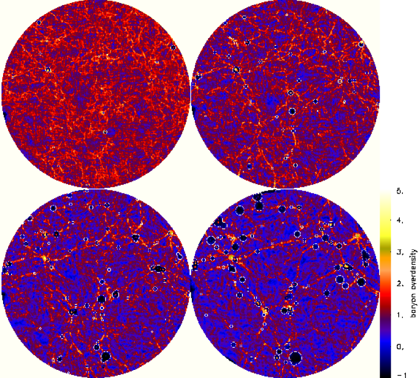
Figure 7: Structure of wind–filled regions as a function of time. The simulations have been realised for M3 assuming $\varepsilon=0.3$ and $K=0.5$. From top to bottom and left to right, the redshifts of the presented snapshots are respectively $z=5$, $z=3$, $z=2$ and $z=1$. The colour coding is the same for all snapshots. The diameter of the region shown is $52h^{-1}$ Mpc in comoving units. The white contours show the extension of winds at the snapshot time, while the dark regions inside the countours are the regions depleted of gas by outflows.

4 Volume Filling Factor of Winds

An estimate of the volume filling factor $f_{v}$ of galactic winds at the redshifts where absorption in quasar spectra is observed can be translated into an estimate of the probability to find disturbances in the Ly$\alpha$ forest due to feedback effects and, in particular, to the presence of wind bubbles. Disturbances here mean regions of the spectra where there are significant variations in the optical depth, due to nongravitational processes stirring the IGM.

Observationally, it is quite challenging to estimate $f_{v}$ with any accuracy. Published estimates range from 0.003 to 40% (Heckman et al. 2001, Cecil et al. 2001, Rauch 2002) at $z\sim 3$. Surely the large scatter is due to the fact that the estimates are mostly indirect and are based on different, perhaps incompatible, assumptions, for example about the geometry of the disturbances.

In Fig. 7 we show an example of the evolution of winds from $z=5$ to $z=1$. A thin slice is cut through the central plane of the simulation and the density distribution of the gas in the slice is shown. The contours indicate the surface of the winds and the black regions inside these contours represent the regions which have been depleted of low density gas by winds. To obtain these simulated distributions, we proceeded as follows. First we recover the density of the gas by applying an SPH smoothing to the distribution of the dark matter particles and by assuming that the distribution of the gas follows the distribution of the dark matter. We then identify the portion of space which is inside one or more bubbles and we consider only those particles that are found inside this region. Particles outside this region are of course not affected by winds. We compute the fraction $x$ of baryons removed from the IGM as the ratio of the total baryon mass of the bubbles plus the galaxies to the total baryonic mass initially associated with the dark matter inside bubbles. We then tag the lowest density particles in the region affected by winds until the same fraction $x$ of the enclosed mass is marked. Finally, we cut a thin slice through the density distribution of the remaining particles in our simulated region, as represented in Fig. 7.

Figure 8: Volume filling factor of winds in M3 as a function of redshift and model parameters. The lines correspond to different parameter choices as in Fig. 1.

We calculate the filling factor of winds by superimposing a 3–dimensional grid on our high resolution region and identifying all the grid points inside winds. Since $f_{v}$ represents the fraction of space occupied by winds, its value is given simply by the ratio between the number of points flagged and the total number of points in the grid. Note that this estimate ignores the mass fraction $1-\varepsilon$ of the IGM which is in “dense clouds” and so avoided entrainment. We use a $512\times 512\times 512$ cubic grid, centered on the centre of mass of the high resolution region and with a side of 52 $h^{-1}$ Mpc, but we limit our analysis to a sphere of diameter 52 $h^{-1}$ Mpc. In principle, a larger region with irregular contours could be identified.

The trends highlighted in paragraph 3.3 are recovered for the behaviour of the volume filling factor, shown in Fig. 8 as a function of time and parameters. The smaller values for $f_{v}$ are clearly related to the cases where fewer mass loaded bubbles are formed and expand into the IGM and viceversa. By varying $K$ and $\varepsilon$, we can obtain a broad range of values of $f_{v}$.

Figure 9: The top panel shows the volume filling factor $f_{v}$ and the overlapping $f_{o}$ of winds for clustered sources and for randomly distributed sources. The results are for our model with $K=0.5$ and $\varepsilon=0.3$, that we assume as our fiducial model here. In the upper panel, the lines represent respectively: (1) thick solid line: fiducial model; (2) dotted line: overlapping for the fiducial model; (3) dashed line: random positions; (4) dashed dotted line: overlapping for the random positions model. In the bottom panel we compare the ratio $f_{o}/f_{v}$ for clustered sources (solid line) and for randomly distributed sources (dashed line).

In the model with $\varepsilon=0.1$ and $K=0.5$, the fraction of volume occupied by winds still increases steadily after $z\sim 2$, but, taking into account the conversion between redshift and cosmic time, less strongly than before. This is probably due to the clustering of the wind sources, which becomes more prominent at lower $z$. As the galaxies cluster and the fraction of the volume occupied by winds and shells increases, the probability of overlapping rises. We do not model the overlapping of winds in a complete way, since our one–dimensional approach does not allow us to take into account the three–dimensional distribution of galaxies and winds on the sky, but we can quantify the overlapping a posteriori. We define $f_{o}$ as the fraction of our simulated volume which is reached by more than one wind. This definition is analogous to the definition of $f_{v}$ and in practice $f_{o}$ can be evaluated simply by counting the fraction of grid points that lie inside two or more winds.

In Fig. 9 we show the results of such a measurement for our model with $\varepsilon=0.3$ and $K=0.5$. Because the galaxies are associated in groups, the wind cavities occupy a smaller fraction of space than they would if they were randomly distributed. At the same time, winds can run into each other much more easily, so the overlapping becomes significant already at high redshift, as is shown in the bottom panel of Fig. 9. The ratio $f_{o}/f_{v}$ represents the fraction of the cavity volume which is reached by two or more winds. While for randomly distributed galaxies overlapping is more uncommon, for clustered galaxies the volume with overlapping winds is already twice as big as in the Poisson case at $z\sim 10$. The probability that winds overlap significantly increases in models with high filling factors.

5 The Wind Mass Budget

A second important indicator of the impact of winds on the surrounding medium is the fraction of intergalactic gas that they affect. This “wind mass fraction” ($f_{m}$, hereafter) is directly dependent on the entrainment fraction and on the mass of gas ejected by the galaxies. $f_{m}$ also depends in a crucial way on the density of the ambient medium crossed by the wind, which, together with the entrainment fraction, determines the accretion rate of gas of winds. In fact, winds expanding into high density regions like filaments or groups may entrain, and therefore affect, much more mass than winds from field galaxies, which are normally embedded in a lower density environment.

We estimate $f_{m}$ as the ratio of the mass in winds to the total mass of IGM in our simulated box. Our results are presented in Fig. 10. While $f_{v}$ is determined only by the physical extension of winds, $f_{m}$ is somewhat more difficult to estimate. In fact, one has to deal correctly with overlapping, which is not treated self–consistently in our semi–analytic prescriptions. To do this, we have to correct approximately for the fact that in our spherical wind model the same material can effectively be swept up two or more times when winds overlap. We first calculate the total mass of IGM inside wind cavities in two different ways, that is from the dark matter particle distribution ($m_{igm,p}$) and from our semi–analytic prescriptions for the distribution of gas around galaxies, given in subparagraph 2.3.5, ($m_{igm,sa}$). The first method reflects the “real” 3–dimensional distribution of matter in our simulated region. We then define $y$ as the ratio between the two, that is $y=m_{igm,p}/m_{igm,sa}$. The bubble mass, defined in equation (2), is the sum of the mass from supernova ejecta (plus the shocked ISM) and of the gas mass entrained along the way $m_{e}$, that is: $m=m_{w}+m_{e}$. The mass of supernova ejecta $m_{w}$ is independent of overlapping effects. Conversely, the entrained mass $m_{e}$ does depend on overlapping and we thus rescale it by the factor $y$ to obtain the actual swept up mass $m^{\prime}_{e}=ym_{e}$. The rescaled wind mass is thus $m^{\prime}=m_{w}+m^{\prime}_{e}$. Finally, we calculate the fraction of IGM mass affected by winds as $f_{m}=m^{\prime}/m_{igm,p}$.

Figure 10: The fraction of IGM mass affected by winds $f_{m}$ as a function of redshift and model parameters. The lines correspond to different parameter choices as in Fig. 1.

The fraction of mass affected by winds $f_{m}$ varies differently from the volume filling factor $f_{v}$ and, in particular, it depends less strongly on the values of the model parameters. The wind mass fraction is lower than 10% at $z>4$, and at $z\sim 2$ is still not higher than 30%. This suggests that winds are unlikely to significantly modify the properties of the Ly$\alpha$ forest at $z\sim 3$ and it is a clear indication that the Ly$\alpha$ forest itself is not entirely modelled by the mechanical effects of feedback. By comparing Fig. 10 and 8, it appears that at low redshifts the winds with low mass loading efficiency have in some cases a large $f_{v}$ and a small $f_{m}$, or viceversa. $f_{m}$ is normally higher than the volume filling factor at any redshift, indicating that although winds do not travel far into the IGM, the effective amount of mass affected may be large. This effect is easy to understand, when one considers that most of the mass in the Universe lies in proximity of high density regions like filaments and clusters and that most of the winds are located in these same regions of space. Only in a few models the volume filling factor reaches higher values than the fraction of mass in winds. In these cases, the actual fraction of intergalactic mass affected by outflows is small even when the winds physically fill a large region of space. This effect is associated with the models with the lowest mass loading efficiencies.

6 The Ejection of Metals

Figure 11: The cumulative distribution of the metal mass in winds at $z=3$ as a function of the stellar mass of the parent galaxies. For comparison, the cumulative distribution of the stellar mass in galaxies is overplotted as a thick line. The other lines correspond to different parameter choices as in Fig. 1.

Which galaxies eject the metals we observe in the IGM? To answer this question, in Fig. 11 we plot the cumulative distribution of metal mass in winds as a function of the stellar mass of the ejecting galaxies for our different models at $z=3$. For comparison, we show the cumulative distribution of the stellar mass in galaxies as a thick straight line.

Different combinations of our model parameters lead to somewhat different shapes for the distribution, but the main conclusion we can draw from Fig. 11 is that at $z=3$ most of the metals are ejected by galaxies with stellar masses in the range $10^{8}-10^{10}$ M_☉, which roughly corresponds to the mass range of dwarf galaxies. Galaxies with stellar masses larger the $10^{10}$ M_☉ or smaller than $10^{8}$ M_☉ do not significantly contribute to the pollution of the IGM. In fact, these galaxies eject altogether about only 20% or less of the metals in winds whose radii exceed the virial radius of the source galaxy. About 80% of the metals come from galaxies with stellar masses in the range $10^{8}<M_{\star}<10^{10}$ M_☉. In all models, galaxies with $10^{9}<M_{\star}<10^{10}$ M_☉ eject about 60% of the metals, and are therefore the main contributors to the pollution. For comparison, about 80% of the total stellar mass in our simulated region lies in galaxies with $10^{8}<M_{\star}<2\cdot 10^{10}$ M_☉. Galaxies with stellar masses larger the $10^{10}$ M_☉ contain about 20% of all the stars, but only in models with inefficient mass loading they contribute up to 30% of the ejected metals.

In Fig. 12 we show the total mass of metals ejected by winds as a function of redshift. This mass increases steadily with decreasing redshift and indicates that galaxies actively contribute to the metal enrichment of the IGM throughout the history of the Universe. The model with the lowest mass loading efficiency ($\varepsilon=0.1$, long dashed line) favours an intense ejection already at high redshift, while all the other models tend to suppress it until more recent times. This behaviour is a consequence of the suppression of winds in models with higher mass loading efficiencies that we discussed in Figs. 4 and 5.

In Fig. 13 we show the mean metallicity of winds in solar units as a function of redshift. This depends on the ratio between the mass entrained from the metal–free IGM and the metal rich gas accreted directly from the wind. We do not find that the metallicity of winds increases with decreasing mass loading efficiency, as it would be reasonable to expect, because the winds forming in models with high mass loading efficiencies are also the ones which travel the shortest distances in our simulations (cfr. Fig. 3), and can therefore entrain the smallest amounts of metal–free ambient medium to dilute their metal content and lower their metallicity. Instead, we observe that the wind metallicity does depend on the parameter $K$, which determines the quantity of ISM blown out of galaxies together with the SN ejecta. This sets directly the metallicity of the wind fluid and, consistently, we find that a low value of $K$ corresponds to metal–poor winds, while a high $K$ to metal–rich ones.

Figure 12: The total mass of metals ejected by winds as a function of redshift and model parameters. The lines correspond to the different parameter choices as in Fig. 1.

6.1 Metals in the Intergalactic Medium

At $z\sim 2$ to 3, recent estimates of the IGM metallicity in regions with densities close to the mean baryon density give values in the range $Z_{IGM}\sim 10^{-3.5}-10^{-2.5}Z_{\odot}$ (Simcoe, Sargent & Rauch 2004, Schaye et al. 2003). We can use the metallicity of our winds to attempt a very rough estimate of the metallicity of the IGM in our simulated region, by multiplying the fraction of intergalactic gas affected by winds by the wind metallicity. As a result, we find that in our simulations the IGM reaches metallicities in the range $Z_{IGM}\sim 10^{-2}-10^{-1.2}Z_{\odot}$ between $z=3$ and $z=2$. The actual value of the metallicity depends on the model parameters and may vary within a factor of a few. The models with $\varepsilon>0.1$ produce the lowest metallicities, while the model with the lowest mass loading efficiency ($\varepsilon=0.1$) predicts the highest metallicity. This can be easily understood, since as we show in Fig. 12 this model predicts the highest amount of metals ejected into the IGM at $z>1$.

Figure 13: The mean metallicity of winds as a function of redshift and model parameters. The lines correspond to different parameter choices as in Fig. 1.

Our estimates of the IGM metallicity are in excess of the observed values by a factor of 10–100, depending on the model. A similar conclusion has recently been formulated by Cen, Nagamine & Ostriker (2004). There are some possible explanations for this: i) our simulated winds may expel more metals into the IGM than actually happens in real galaxies; ii) the metals in winds do not effectively pollute the IGM uniformly, so that different concentrations of metals could be found at different locations in space; and finally, iii) the ejected metals may not be efficiently mixed into the observed “cold” gas, and therefore may not be detectable in absorption in the Ly$\alpha$ forest.

While our models might overestimate the total amount of mass and metals ejected by galaxies by a factor of up to a few, it is unlikely that such a correction would change our conclusion that the mean IGM metallicity is higher than observations of the Ly$\alpha$ forest suggest.

Of course, regions affected by winds may have metallicities of order $Z_{wind}$, while unaffected regions would likely mantain their pristine chemical composition. Other mechanisms different from galactic winds may in principle pre–enrich the lowest density regions of the Universe at earlier times, like e.g. Pop III stars or pregalactic outflows. On the other hand, the high metallicities predicted by our simulations in the outskirts of galaxies may explain why systematic velocity shifts of few hundred km s^-1 between Ly$\alpha$ and metal absorption lines have been found in several quasar spectra.

Alternatively, the discrepancy between our estimate of the IGM metallicity and the observed values cited above may be explained by the non–detection of part of the intergalactic metals. But why should we be unable to detect these metals? The C IV and O VI detected in the spectra of quasars reside in a photoionised gas at temperatures of about $10^{4}-10^{5}$ K. For higher temperatures, collisional ionisation becomes efficient, so that carbon and oxygen are fully ionised and do not absorb the UV photons anymore. The temperature of winds may thus be a key factor to determine the observability of their metal content in absorption.

In our model, we find that at $z=3$ a large fraction of the winds that have escaped the potential wells of haloes have temperatures lower than about $10^{6}$ K. If the wind temperature drops below about $10^{5.5}$ K, photoionisation replaces collisional ionisation as the main ionisation mechanism and cooled shells could produce C IV and O VI absorption. In most cases, pressure driven bubbles do have temperatures higher than $10^{6}$ K and no metal absorption could take place. In Fig. 14 we plot the fraction of the metal mass transported by winds with temperatures higher than $10^{5.5}$ K, which therefore would not produce any observable absorption in the spectra of quasars. Although this result is strongly parameter dependent, it is clear that at $1\lesssim z\lesssim 5$ a significant fraction of the metals resides in a hot gas that would leave no footprint in the Ly$\alpha$ forest. This result may support the idea that the IGM is enriched to a higher level than Ly$\alpha$ observations can prove, but that the metals blown out of galaxies by galactic winds are in many cases too hot to produce any detectable absorption in the spectra of quasars.

Figure 14: The fraction of metal mass in winds with $T>10^{5.5}$ K as a function of redshift and model parameters. The lines correspond to different parameter choices as in Fig. 1.

Gas at temperatures as high as $10^{7}$ K is expected to emit radiation in the X–ray band and one would expect to find X–ray emission in the IGM not associated with jets or collapsed objects. Indeed, X–ray emission from highly ionised metal species (O VIII and Ne X) in a warm–hot IGM (WHIGM) may have been recently discovered by CHANDRA (e.g. Nicastro et al. 2002, McKernan et al. 2003). This hot gas may be shock–heated by galactic winds as well as from the process of structure formation or jets from active galaxies. If the first case is true, this gas may represent the hot metal enriched gas in our bubbles, which is too highly ionised to produce absorption in the Ly$\alpha$ forest.

7 The effect of mass resolution

We want now to investigate the effect of the resolution in mass of our N–body simulations in determining the volume filling factor and the fraction of IGM mass affected by winds. To do this, we compare the results obtained from our four sets of simulations with increasing mass resolution. While a large population of dwarf galaxies is already forming at $z\lesssim 20$ in M3, only a few objects are assembling in M2 at the same epoch and in the lower resolution runs M1 and M0 the first galaxies appear only at $z<15$ and $z<7$, respectively. The total number of galaxies in M3 is five times as large as in M2 at $z=0$ and the number of galaxies with winds two times as large.

In Fig. 15 we show the volume filling factor (top panel) and the fraction of mass affected by winds (lower panel) in the M1, M2 and M3 simulation sets. The results are shown for a model with parameters $\varepsilon=0.3$ and $K=0.5$. We find that at high redshift $f_{v}$ and $f_{m}$ strongly depend on the mass resolution and on the ability to resolve galaxies which form in haloes with total masses of about $10^{9}-10^{10}$ M_☉. These galaxies, only resolved in M3, include galaxies with both low and intermediate stellar masses, field galaxies and satellites.

Figure 15: Dependence of the volume filling factor $f_{v}$ (upper panel) and of the fraction of mass affected by winds $f_{m}$ (lower panel) on the mass resolution of the dark matter N–body simulations. The results are for a model with parameters $\varepsilon=0.3$ and $K=0.5$ and the lines represent respectively three of our simulation sets: (1) solid line: M3, $M_{p}=1.7\cdot 10^{8}h^{-1}$ M_☉; (2) dotted line: M2, $M_{p}=9.5\cdot 10^{8}h^{-1}$ M_☉; (3) dashed line: M1, $M_{p}=4.8\cdot 10^{9}h^{-1}$ M_☉. The large galaxies resolved in M0 do not give any significant contribution at any redshift.

At $z\sim 0$ the results for the different sets of simulations converge. This is an indication of the fact that dwarf galaxies are mainly responsible for the pollution of the IGM at high redshift, but that their relative contribution becomes smaller at very low redshift, when more massive galaxies become the main sources of powerful winds and can account for most of the mass and metals ejected into the IGM.

Despite the convergence of the global star formation in our simulated region (cfr. Subsection 2.2), the star formation history of single objects may vary from M2 to M3. This determines a different evolution of winds with time: in M2 bubbles tend to form at later times and expand faster than in M3, as a consequence of a more intense star formation activity concentrated at later times and triggered by a faster accretion of gas onto the fewer galaxies. When bubbles form in M2, the dark matter haloes in which they expand already possess total masses larger than the haloes in M3, but the larger energy provided by star formation often compensates for the increased gravitational attraction. This is why the convergence of the curves in Fig. 15 is not exact, but may differ by a small factor, generally not larger than a few percent.

One may ask if objects with stellar masses lower than about $10^{7}$–$10^{8}$ M_☉ might give a substantial contribution to the pollution of the IGM at redshifts where larger objects have not yet assembled. Indeed, Madau, Ferrara & Rees (1999) claim that the IGM has been polluted by outflows from pregalactic objects, with total masses well below $10^{8}-10^{9}$ M_☉. In principle, winds may escape very easily the shallow potential wells of such objects, if the energy input from star formation is high enough to accelerate the accreted mass to velocities larger than the escape velocities of their haloes. At lower redshifts, the evolution of objects with total masses lower than $10^{9}$ M_☉ may be affected by feedback effects that inhibite their star formation activity (e.g. Haiman, Rees & Loeb 1997, Mac Low & Ferrara 1999). As a result, these objects would be unable to blow winds, making their contribution to the pollution of the low redshift IGM negligible with respect to other galaxy populations with higher stellar masses. Unfortunately, our simulations do not have sufficient resolution to follow the evolution of these objects. However, in the light of the results displayed in Fig. 15, we believe that such low stellar mass galaxies would not significantly change our conclusions.

8 Conclusions

We have presented semi–analytic simulations of galaxy formation in a cosmological context, which include the physics of galactic winds. The semi-analytic prescriptions are applied to high resolution N–body simulations of a typical “field” region of the Universe.

The results of our model can be quite accurately interpreted as a consequence of the mass loading efficiency of winds. The mass accumulated in bubbles is directly linked to the amount of mass entrained from the ambient medium, set by the parameter $\varepsilon$, and the ultimate fate of winds is strongly dependent on this swept–up mass. Bubbles that load little mass from the surrounding medium can escape the gravitational potential well of their host haloes more efficiently at every redshift. These bubbles are mostly composed of metal rich supernova ejecta and shocked ISM and need to spend little of their energy to accelerate the accreted gas. Since most of the energy injected by the starburst is available to power the expansion of the bubble, these winds have the highest probability to escape the gravitational attraction of haloes and expand into the IGM. The formation of highly mass loaded winds is instead suppressed in all kinds of galaxies, although the suppression is particularly strong in galaxies with $M_{\star}\lesssim 10^{9}$ M_☉. This is because the energy provided by star formation is not sufficient to overcome the ram pressure of the infalling material which adds to the gravitational pull of the galaxy.

Our estimates of the volume filling factor of winds (Section 4) and of the fraction of IGM mass affected by winds (Section 5) suggest that galactic outflows are unlikely to significantly modify the properties of the Ly$\alpha$ forest. No obvious correlation is found between $f_{m}$ and $f_{v}$. The volume filling factor is clearly dependent on the mass loading efficiency of bubbles, with low values of $f_{v}$ associated with highly mass loaded bubbles and viceversa. The fraction of IGM mass affected by winds is usually comparable to the volume filling factor. Only in models with high mass loading efficiency we find that $f_{m}>f_{v}$, which implies that the actual fraction of intergalactic mass affected by outflows may be large even when the winds physically fill a small region of space. This is a consequence of the clustering of matter on large scales and of the fact that galaxies form in high density regions, where their winds can sweep up a larger amount of material than they would if they were expanding inside a low density region.

The efficiency of winds in seeding the IGM with metals is investigated in section 6. Galaxies with $M_{\star}\lesssim 10^{9}$ M_☉ play a role in the chemical enrichment of the IGM only at very high redshifts, when larger objects have not yet assembled. At $z=3$ most of the metals are ejected by galaxies with $10^{9}\lesssim M_{\star}\lesssim 10^{10}$ M_☉, while galaxies with $M_{\star}\gtrsim 10^{10}$ M_☉ contribute only about 10%–20% of the ejected metals. The result that metals are mostly ejected by relatively small galaxies qualitatively agrees with the predictions of e.g. Theuns, Mo & Schaye (2001), Theuns et al. (2002), Thacker, Scannapieco & Davis (2002).

Our estimates of the mean metallicity of the IGM are significantly higher than the observed values at $z\sim 1$ to $z\sim 5$ and we have argued that metals in the IGM might not be observable in absorption in the spectra of quasars because of the high temperatures of winds. In a forthcoming paper we will discuss the possibility of finding observable signatures of cooled wind shells in the Ly$\alpha$ forest.

References

- Adelberger et al. (2003) Adelberger K.L., Steidel C.C., Shapley A.E., Pettini M., 2003, ApJ, 584, 45
- Aguirre et al. (2001) Aguirre A., Hernquist L., Schaye J., Katz N., Weinberg D.H., Gardner J. 2001, ApJ, 561, 521
- Cecil, Bland-Hawthorn & Veilleux (2002) Cecil G., Bland-Hawthorn J., Veilleux S., 2002, ApJ, 576, 745
- Cecil et al. (2001) Cecil G., Bland-Hawthorn J., Veilleux S., Filippenko A.V., 2001, ApJ, 555, 338
- Cen, Nagamine & Ostriker (2004) Cen R., Nagamine K., Ostriker J.P., 2004, pre–print astro–ph/0407143
- Ciardi, Stoehr and White (2003) Ciardi B., Stoehr F., White S.D.M., 2003, MNRAS, 343, 1101
- Cowie et al. (1995) Cowie L.L., Songaila A., Kim T.–S., Hu E.M., 1995, AJ, 109, 1522
- Croft et al. (2002) Croft R.A.C., Hernquist L., Springel V., Westover M., White M., 2002, ApJ, 580, 634
- Dekel & Silk (1986) Dekel A., Silk J., 1986, ApJ, 303, 39
- Efstathiou (2000) Efstathiou G., 2000, MNRAS 317, 697
- Ellison et al. (1999) Ellison S.L., Lewis G.F., Pettini M., Chaffee F.H., Irwin M.J., 1999, ApJ, 520, 456
- Frye, Broadhurst & Benitez (2002) Frye B,. Broadhurst T., Benitez N. 2002, ApJ, 568, 558
- Haiman, Rees & Loeb (1997) Haiman Z., Rees M.J., Loeb A., 1997, ApJ, 476, 458
- Heckman, Armus & Miley (1990) Heckman T.M., Armus L., Miley G.K., 1990, ApJSS, 74, 833
- Heckman et al. (2000) Heckman T.M., Lehnert M.D., Strickland D.K., Armus L. 2000, ApJS, 129, 493
- Heckman et al. (2001) Heckman T.M., Sembach K.R., Meurer G.R., Strickland D.K., Martin C.L., Calzetti D., Leitherer C., 2001, ApJ, 554, 1021
- Hoopes et al. (2003) Hoopes C.G., Heckman T.M., Strickland D.K., Howk J.C., 2003, ApJL, 596, 175
- Jenkins et al. (2001) Jenkins A., Frenk C.S., White S.D.M., Colberg J.M., Cole S., Evrard A.E., Couchman H.M.P., Yoshida N., 2001, MNRAS, 321, 372
- Kauffmann et al. (1999) Kauffmann G., Colberg J.M., Diaferio A., White S.D.M. 1999, MNRAS, 303, 188
- Madau, Ferrara & Rees (1999) Madau P., Ferrara A., Rees M.J., 2001, ApJ, 555, 92
- Martin (1999) Martin C.L. 1999, ApJ, 513, 156
- Mac Low & Ferrara (1999) Mac Low M.–M., Ferrara A., 1999, ApJ, 513, 142
- McKee & Ostriker (1977) McKee C.F., Ostriker J.P. 1977, ApJ, 218, 148
- McKernan et al. (2003) McKernan B., Yaqoob T., Mushotzky R., George I.M., Turner T.J., 2003, ApJL, 598, 83
- Navarro, Frenk & White (1996) Navarro J.F., Frenk C.S., White S.D.M., 1996, ApJ, 462, 563
- Nicastro et al. (2002) Nicastro F., Zezas A., Drake J., Elvis M., Fiore F., Fruscione A., Marengo M., Mathur S., Bianchi S., 2002, ApJ, 573, 157
- Ostriker & McKee (1988) Ostriker J.P., McKee C.F. 1988, Rev.Mod.Phys. 60, 1
- Pettini et al. (2002) Pettini M., Rix S., Steidel C., Hunt M.P., Shapley A.E., Adelberger K., 2002, Ap&SS, 281, 461
- Phillips (1993) Phillips A.C., 1993, AJ, 105, 486
- Rauch (2002) Rauch M., 2002, ASP Conference Proc. Ed. J.S. Mulchaey & J. Stocke, 254, 140
- Schaye et al. (2003) Schaye J., Aguirre A., Kim T.-S., Theuns T., Rauch M., Sargent W. L. W., 2003, ApJ, 596, 768
- Schaye et al. (2000) Schaye J., Rauch M., Sargent W. L. W., Kim T.-S., 2000, ApJL, 541, 1
- Shu, Mo & Mao (2003) Shu C., Mo H.J., Mao S. 2003, pre–print astro–ph/0301035
- Simcoe, Sargent & Rauch (2004) Simcoe R.A., Sargent W.L.W., Rauch M., 2004, ApJ, 606, 92
- Springel & Hernquist (2003) Springel V., Hernquist L. 2003, MNRAS, 339, 312
- Springel et al. (2001) Springel V., White S.D.M., Tormen G., Kauffmann G. 2001, MNRAS, 328, 726
- Springel, Yoshida & White (2001) Springel V., Yoshida N., White S.D.M. 2001, New Astronomy, 6, 79
- Stoehr (2003) Stoehr F., 2003, PhD Thesis, Ludwig Maximilian Universität, München
- Strickland & Stevens (2000) Strickland D.K., Stevens I.R., 2000, MNRAS, 314, 511
- Sugai, Davies & Ward (2003) Sugai H., Davies R.I., Ward M.J., 2003, ApJ, 584, 9
- Sutherland & Dopita (1993) Sutherland R.S., Dopita M.A., 1993, ApJSS, 88, 253
- Thacker, Scannapieco & Davis (2002) Thacker R.J., Scannapieco E., Davis M., 2002, ApJ, 581, 836
- Theuns, Mo & Schaye (2001) Theuns T., Mo H.J., Schaye J. 2001, MNRAS, 321, 450
- Theuns et al. (2002) Theuns T., Viel M., Kay S., Schaye J., Carswell R.F., Tzanavaris P. 2002, ApJL, 578, 5
- Tormen, Bouchet & White (1997) Tormen G., Bouchet F.R., White S.D.M. 1997, MNRAS, 286, 865
- Walter, Weiss & Scoville (2002) Walter F., Weiss A., Scoville N., 2002, ApJ, 580, 21
- Yoshida, Sheth & Diaferio (2001) Yoshida N., Sheth R.K., Diaferio A. 2001, MNRAS, 328, 669