On the origin of H₂CO abundance enhancements in low-mass protostars

High angular resolution H₂CO 218 GHz line observations have been carried out toward the low-mass protostars IRAS~16293–2422 and L1448–C using the Owens Valley Millimeter Array at $\sim$2$\arcsec$ resolution. Simultaneous 1.37 mm continuum data reveal extended emission which is compared with that predicted by model envelopes constrained from single-dish data. For L1448–C the model density structure works well down to the 400 AU scale to which the interferometer is sensitive. For IRAS 16293–2422, a known proto-binary object, the interferometer observations indicate that the binary has cleared much of the material in the inner part of the envelope, out to the binary separation of $\sim$800 AU. For both sources there is excess unresolved compact emission centered on the sources, most likely due to accretion disks $\lesssim$200 AU in size with masses of $\gtrsim$0.02 M_⊙ (L1448–C) and $\gtrsim$0.1 M_⊙ (IRAS 16293–2422). The H₂CO data for both sources are dominated by emission from gas close to the positions of the continuum peaks. The morphology and velocity structure of the H₂CO array data have been used to investigate whether the abundance enhancements inferred from single-dish modelling are due to thermal evaporation of ices or due to liberation of the ice mantles by shocks in the inner envelope. For IRAS 16293–2422 the H₂CO interferometer observations indicate the presence of large scale rotation roughly perpendicular to the large scale CO outflow. The H₂CO distribution differs from that of C¹⁸O, with C¹⁸O emission peaking near MM1 and H₂CO stronger near MM2. For L1448–C, the region of enhanced H₂CO emission extends over a much larger scale $>$1^′′ than the radius of $50-100$ K ($0\aas@@fstack{\prime\prime}6-0\aas@@fstack{\prime\prime}15$) where thermal evaporation can occur. The red-blue asymmetry of the emission is consistent with the outflow; however the velocities are significantly lower. The H₂CO $3_{22}-2_{21}/3_{03}-2_{02}$ flux ratio derived from the interferometer data is significantly higher than that found from single-dish observations for both objects, suggesting that the compact emission arises from warmer gas. Detailed radiative transfer modeling shows, however, that the ratio is affected by abundance gradients and optical depth in the $3_{03}-2_{02}$ line. It is concluded that a constant H₂CO abundance throughout the envelope cannot fit the interferometer data of the two H₂CO lines simultaneously on the longest and shortest baselines. A scenario in which the H₂CO abundance drops in the cold dense part of the envelope where CO is frozen out but is undepleted in the outermost region provides good fits to the single-dish and interferometer data on short baselines for both sources. Emission on the longer baselines is best reproduced if the H₂CO abundance is increased by about an order of magnitude from $\sim$$10^{-10}$ to $\sim$$10^{-9}$ in the inner parts of the envelope due to thermal evaporation when the temperature exceeds $\sim$50 K. The presence of additional H₂CO abundance jumps in the innermost hot core region or in the disk cannot be firmly established, however, with the present sensitivity and resolution. Other scenarios, including weak outflow-envelope interactions and photon heating of the envelope, are discussed and predictions for future generation interferometers are presented, illustrating their potential in distinguishing these competing scenarios.

1 Introduction

Recent observational studies have shown that the inner ($<$ few hundred AU) envelopes of low-mass protostars are dense ($\gtrsim$10⁶ cm^-3) and warm ($\gtrsim$80 K) (Blake et al. 1994; Ceccarelli et al. 2000a; Jørgensen et al. 2002; Schöier et al. 2002; Shirley et al. 2002), as expected from scaling of high-mass protostars (Ceccarelli et al. 1996; Ivezić & Elitzur 1997). In high-mass objects, these warm and dense regions are known to have a rich chemistry with high abundances of organic molecules due to the thermal evaporation of ices (e.g., Blake et al. 1987; Charnley et al. 1992). Detailed modeling of multi-transition single-dish lines toward the deeply embedded low-mass protostar IRAS 16293–2422 has demonstrated that similar enhancements of molecules like H₂CO and CH₃OH can occur for low-mass objects (van Dishoeck et al. 1995; Ceccarelli et al. 2000b; Schöier et al. 2002). Recently, Maret et al. (2004) have suggested that this is a common phenomenon in low-mass protostars. The location at which this enhancement occurs is consistent with the radius at which ices are expected to thermally evaporate off the grains ($T\gtrsim 90$ K). Moreover, large organic molecules have recently been detected toward IRAS 16293–2422 (Cazaux et al. 2003), showing that low-mass hot cores may have a similar chemical complexity as the high-mass counterparts in spite of their much shorter timescales (Schöier et al. 2002).

Alternatively, shocks due to the interaction of the outflow with the inner envelope can liberate grain mantle material over a larger area than can thermal heating. Additionally, the bipolar outflow will excavate a biconical cavity in the envelope through which UV- and X-ray photons can escape. The back scattering of such photons into the envelope by low-density dust in the cavity can significantly heat the envelope surrounding the cavity (e.g., Spaans et al. 1995). This would produce regions of warm gas ($\sim$100 K) in the envelope on much larger scales than otherwise possible. High angular resolution observations are needed to pinpoint the origin of the abundance enhancements and distinguish between these various scenarios.

We present here observations of H₂CO toward two low-mass protostars, IRAS 16293–2422 and L1448–C (also known as L1448–mm), at 218 GHz (1.4 mm) using the Owens Valley Radio Observatory (OVRO) Millimeter Array at $\sim$2$\arcsec$ resolution. The frequency setting includes the $3_{03}\rightarrow 2_{02}$ and $3_{22}\rightarrow 2_{21}$ H₂CO lines, whose ratio is a measure of the gas temperature of the circumstellar material. Both IRAS 16293–2422 and L1448–C are deeply embedded class 0 protostars (André et al. 1993) which drive large scale ($\sim$ arcmin) bipolar outflows (Walker et al. 1988; Mizuno et al. 1990; Bachiller et al. 1990, 1991; Stark et al. 2004). For other low-mass objects, molecules such as SiO are clearly associated with the outflow (e.g., L1448: Guilloteau et al. 1992; NGC 1333 IRAS4: Blake 1995), whereas optically thick lines from other species such as HCO⁺ and HCN are found to ‘coat’ the outflow walls (e.g., B5 IRS1: Langer et al. 1996; L1527 and Serpens SMM1: Hogerheijde et al. 1997, 1999). The extent of this emission can be larger than $10\arcsec$, which should be readily distinguishable from the $\sim$1$\arcsec$ hot inner envelope with current interferometers.

Previous millimeter aperture synthesis observations of IRAS 16293–2422 have revealed two compact components coincident with radio continuum emission, indicative of a protobinary source (Mundy et al. 1990, 1992). The line emission of 10 molecular species at $\sim$5$\arcsec$ resolution reveals that there is a red-blue asymmetry indicative of rotation perpendicular to the outflow direction (Schöier et al., in prep.). The morphology of the emission picked up by the interferometer suggests that it may be produced in regions of compressed gas as a result of interaction between the outflow and the envelope. Previous data on L1448–C show a compact continuum source at millimetre wavelengths and that SiO is a good tracer of the large velocity outflow associated with this source (Guilloteau et al. 1992).

Since most of the extended emission is resolved out by the interferometer, a good physical and chemical model of the envelope is a prerequisite for a thorough interpretation of the aperture synthesis data. In recent years, much progress has been made in obtaining reliable descriptions of the density and temperature structures in the dusty envelopes around young stellar objects, based on thermal continuum emission (Chandler & Richer 2000; Hogerheijde & Sandell 2000; Motte & André 2001; Jørgensen et al. 2002; Schöier et al. 2002; Shirley et al. 2002). The physical structures of IRAS 16293–2422 and L1448–C have recently been derived from single-dish continuum observations, with the results summarized in Table 1 (Jørgensen et al. 2002; Schöier et al. 2002).

In §3, we first test the validity of these envelope models at the small scales sampled by the continuum interferometer data. In §4, the H₂CO results are presented and analyzed. For IRAS 16293–2422, C¹⁸O observations are also available. This is followed by a discussion on the origin of H₂CO and estimates for what future generation telescopes might reveal in §5 and by conclusions in §6.

Table 1: Source and envelope parameters for IRAS 16293–2422 and L1448–C

$$\begin{array}[]{p{0.61\linewidth}cc}\hline\cr\hline\cr\vskip 3.0pt plus 1.0pt minus 1.0pt\cr&\mathrm{IRAS\ 16293}^{a}&\mathrm{L1448}^{b}\\ \hline\cr\vskip 3.0pt plus 1.0pt minus 1.0pt\cr Distance, $D$ (pc)&160&220\\ Luminosity, $L$ (L${}_{\sun}$)&27&5\\ Inner radius, $r_{\mathrm{i}}$ (AU)&32.1&9.0\\ Outer radius, $r_{\mathrm{e}}$ (10${}^{4}$\,AU)&0.80&0.81\\ Density power law index, $\alpha$&1.7&1.4\\ Density at 1000\,AU, $n_{0}$(H${}_{2}$) ($10^{6}$\,cm${}^{-3}$)&6.7&0.75\\ Column density${}^{c}$, $N(\mathrm{H}_{2})$ (10${}^{24}$\,cm${}^{-2}$)&1.6&0.17\\ Envelope mass${}^{c}$, $M_{\mathrm{env}}$ (M${}_{\sun}$)&5.4&0.93\\ \hline\cr\vskip 3.0pt plus 1.0pt minus 1.0pt\cr${}^{a}$ From \cite[citet]{\@@bibref{Authors Phrase1YearPhrase2}{Schoeier02}{\@@citephrase{(}}{\@@citephrase{)}}}\\ ${}^{b}$ From \cite[citet]{\@@bibref{Authors Phrase1YearPhrase2}{Joergensen02}{\@@citephrase{(}}{\@@citephrase{)}}}\\ ${}^{c}$ Within the outer radius $r_{\mathrm{e}}$\\ \end{array}$$

2 Observations and data reduction

2.1 Interferometer data

The two protostars IRAS 16293–2422 ($\alpha_{2000}=16^{\mathrm{h}}32^{\mathrm{m}}22\aas@@fstack{s}8$, $\delta_{2000}=-24{\degr}28{\arcmin}33\aas@@fstack{\prime\prime}0$) and L1448–C ($\alpha_{2000}=3^{\mathrm{h}}25^{\mathrm{m}}38\aas@@fstack{s}8$, $\delta_{2000}=30{\degr}44{\arcmin}05\aas@@fstack{\prime\prime}0$) were observed with the Owens Valley Radio Observatory (OVRO) Millimeter Array between September 2000 and March 2002. The H₂CO $3_{03}\rightarrow 2_{02}$ and $3_{22}\rightarrow 2_{21}$ line emission at 218.222 and 218.475 GHz, respectively, was obtained simultaneously with the continuum emission at 1.37 mm. IRAS 16293–2422 was observed in the L and E configurations, while L1448–C was observed in the C, L and H configurations, corresponding to projected baselines of $8-80$ and $8-120$ k$\lambda$, respectively. The complex gains were calibrated by regular observations of the quasars NRAO 530 and 1622–253 for IRAS 16293–2422 and 0234$+$285 for L1448–C, while flux calibration was done using observations of Uranus and Neptune for each track, both using the MMA package developed for OVRO data by Scoville et al. (1993). The subsequent data-reduction and analysis was performed using MIRIAD (Sault et al. 1995).

Further reduction of the data was carried out using the standard approach by flagging clearly deviating phases and amplitudes. The continuum data were self-calibrated and the resulting phase corrections were applied to the spectral line data, optimizing the signal-to-noise. The natural-weighted continuum observations for IRAS 16293–2422 and L1448–C have typical 1$\sigma$ noise levels better than 20 and 3 mJy beam^-1 with beam sizes of 3$\aas@@fstack{\prime\prime}$9$\times$1$\aas@@fstack{\prime\prime}$9 and 2$\aas@@fstack{\prime\prime}$6$\times$2$\aas@@fstack{\prime\prime}$3, respectively. The relatively high noise levels for IRAS 16293–2422 reflect the low elevation at which this source is observable from Owens Valley, which both increases the system temperatures and decreases the time available per transit. The data were then CLEANed (Högbom 1974) down to the 2$\sigma$ noise level.

For IRAS 16293–2422 additional archival C¹⁸O $J=2\rightarrow 1$ line data obtained in 1993 using the OVRO array are presented, which were reduced in the same way as described above.

2.2 Single-dish data

It is well-known that the millimeter aperture synthesis observations lack sensitivity to extended emission due to discrete sampling in the $(u,v)$ plane and, in particular, missing short-spacings. In order to quantify this single-dish observations were performed using the James Clerk Maxwell Telescope (JCMT). The continuum data are taken largely from the JCMT archive and have been presented in Schöier et al. (2002) and Jørgensen et al. (2002). For H₂CO, a 25-point grid centered on the adopted source position and sampled at 10$\arcsec$ spacing was obtained in September 2002 for IRAS 16293–2422, with both H₂CO 218 GHz lines covered in a single spectral setting. The observations were obtained in a beam-switching mode using a $180\arcsec$ chop throw. The data were calibrated using the chopper-wheel method and the resulting antenna temperature was converted into main-beam brightness temperature, $T_{\mathrm{mb}}$, using the main-beam efficiency $\eta_{\mathrm{mb}}=0.69$. For L1448–C, a single spectrum at the source position was taken that includes both transitions.

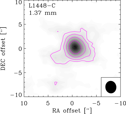
Figure 1: OVRO interferometer maps of the 1.37 mm continuum emission toward L1448–C. Contours start at 9 mJy beam^-1 and the first contour corresponds to the ‘2$\sigma$’-level as estimated from the maps. Each successive contour is a multiple of two of the preceding value. The peak value is 0.13 Jy beam^-1 and the synthesized beam in this and subsequent images is depicted by the filled ellipse in the lower-right corner.

3 Continuum emission: disk and envelope structure

3.1 L1448–C

In Fig. 1, the 221.7 GHz (1.37 mm) continuum emission toward L1448–C is presented. Only a single compact component is seen, with faint extended emission. The total continuum flux density at 1.37 mm observed with OVRO is 0.32 Jy, only 35% of the flux observed by Motte & André (2001) (0.9 Jy) at 1.3 mm using the IRAM 30 m telescope. The compact component, located at ($-0\aas@@fstack{\prime\prime}6$, $0\aas@@fstack{\prime\prime}2$) from the pointing centre, has been fitted with a Gaussian in the ($u,v$) plane, resulting in an estimated size of 1$\aas@@fstack{\prime\prime}$0$\times$0$\aas@@fstack{\prime\prime}$6 and an upper limit to the diameter of $\sim$170 AU for the adopted distance of 220 pc.

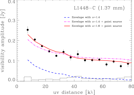
Figure 2: Visibility amplitudes of the observed 1.37 mm continuum emission obtained at OVRO towards L1448–C as functions of the projected baseline length, binned to 5 k$\lambda$, from the phase center, taken to be at ($-0\aas@@fstack{\prime\prime}6,0\aas@@fstack{\prime\prime}2$). The observations are plotted as filled symbols with 1$\sigma$ error bars. The dotted histogram represents the zero-expectation level. Also shown are predictions based on a realistic physical model for the source (Jørgensen et al. 2002), with the same ($u,v$) sampling as the observations (see text for details). Unresolved compact emission, presumably from a circumstellar disk, must be added to that from the envelope to produce an acceptable fit.

Jørgensen et al. (2002) determined the actual temperature and density distribution of the circumstellar envelope of L1448–C from detailed modeling of the observed continuum emission (see Table 1). In addition to the spectral energy distribution (SED), resolved images at 450 and 850 $\mu$m obtained with the SCUBA bolometer array at the JCMT were used to constrain the large scale envelope structure. The interferometer data constrain the envelope structure at smaller scales ($\sim$2$\arcsec$) than the JCMT single-dish data ($\sim$10-20$\arcsec$). In order to investigate whether this envelope model can be reconciled with the flux picked up by the interferometer, the same ($u,v$) sampling was applied to the predicted brightness distribution at 1.37 mm from the model envelope.

Fig. 2 compares the observed visibility amplitudes of L1448–C with the model predictions. First, it is clear that the envelope alone cannot reproduce the data, but that an unresolved compact source, presumably the disk, needs to be added. The combination of this point source and the best fit envelope model of Jørgensen et al. (2002) with a density structure falling off as $r^{-\alpha}$, where $\alpha=1.4$, dramatically improves the fit to the visibilities in the $(u,v)$ plane. A slightly steeper density structure of $\alpha=1.6$ is preferred by the interferometer data. Given the mutual uncertainties of $\pm 0.2$ in $\alpha$ these results are still in good agreement with each other and with those of Shirley et al. (2002), who found a slope $\alpha=1.7$ in their analysis for a somewhat larger ($r_{e}=45000$ AU) envelope. The remaining point source flux for L1448–C is estimated to be 100 and 75 mJy when $\alpha$ is taken to be 1.4 and 1.6, respectively. This is $\sim 10$% of the total single-dish source flux. The impact of changing different envelope parameters such as density slope and location of inner envelope radius was tested in Jørgensen et al. (2004a), for the embedded low-mass protostar NGC 1333–IRAS2A, and found to lead to an uncertainty of about $\pm 25$% on the derived point source flux.

The point source flux estimated here at 1.37 mm agrees very well with the spectral index of $1.84\pm 0.08$ found from other mm and cm wavelength observations (Curiel et al. 1990; Guilloteau et al. 1992; Looney et al. 2000; Reipurth et al. 2002) as shown in Fig. 3. The quoted standard deviation is based on assuming a 20% uncertainty in all the fluxes. Similarly, Jørgensen et al. (2004a) found a spectral index of 1.9 for the point source associated with the low-mass protostar NGC 1333–IRAS2A. The spectral index is consistent with optically thick thermal emission and its favoured origin is that from an unresolved accretion disk.

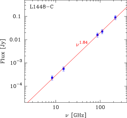
Figure 3: Continuum flux observations of the compact emission toward L1448–C (squares with error bars). The solid line shows a fit to the data using $F\propto\nu^{\beta}$, where $\beta=1.84\pm 0.08$ is the spectral index.

Assuming the point source emission to be thermal the mass of the compact region can be estimated from

$$M=\frac{F_{\nu}\Psi D^{2}}{\kappa_{\nu}B_{\nu}(T_{\mathrm{d}})}\left(\frac{\tau_{\nu}}{1-e^{-\tau_{\nu}}}\right),$$ (1)

where $F_{\nu}$ is the flux, $\Psi$ is the gas-to-dust ratio (assumed to be equal to 100), $D$ is the distance, $\kappa_{\nu}$ is the dust opacity, $B_{\nu}$ is the Planck function at a characteristic dust temperature $T_{\mathrm{d}}$ and $\tau_{\nu}$ is the optical depth. The adopted dust opacity at 1.37 mm, 0.8 cm² g^-1, is extrapolated from the opacities presented by Ossenkopf & Henning (1994) for grains with thin ice mantles. These opacities were used also in the radiative transfer analysis of the envelope. For a dust temperature in the range $100-40$ K, the estimated disk mass in the optically thin limit is $0.016-0.042$ M_⊙ when a point source flux of 75 mJy is used. This should be treated as a lower limit since the emission is likely to be optically thick at 1.37 mm, as suggested by the spectral index.

It is difficult to estimate accurate disk masses for deeply embedded sources since it involves a good knowledge about the envelope structure, in addition to, e.g., the disk temperature. For more evolved protostars where the confusion with the envelope is less problematic, disk masses of $\sim$0.01 - 0.08 M_⊙ are derived (e.g., Looney et al. 2000; Mundy et al. 2000), comparable to the values found here.

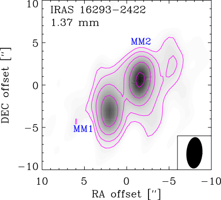
Figure 4: OVRO interferometer maps of the continuum emission at 1.37 mm towards IRAS 16293–2422. Contours start at 60 mJy beam^-1 and the first contour corresponds to the ‘2$\sigma$’-level as estimated from the maps. Each successive contour is a multiple of two of the preceding value. The emission peaks at 0.82 and 1.1 Jy beam^-1 at MM1 and MM2, respectively.

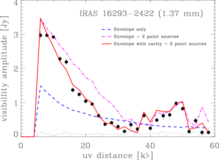
Figure 5: Visibility amplitudes of the observed 1.37 mm emission obtained at OVRO towards IRAS 16293–2422 as functions of the projected baseline length, binned to 2 k$\lambda$, from the phase center, taken to be at (0,0). The observations are plotted as filled symbols with 1$\sigma$ error bars. The dotted histogram represents the zero-expectation level. Also shown are predictions based on a realistic physical model for the source (Schöier et al. 2002), with the same ($u,v$) sampling as the observations (see text for details). Unresolved compact emission, presumably from two circumstellar disks, needs to be added to that emanating from the envelope in order to obtain an acceptable fit. A model envelope with a cavity (solid line), in addition to the unresolved compact emission, is shown to best reproduce the observations.

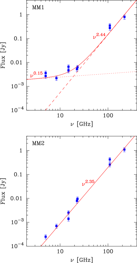
Figure 6: Continuum flux observations of the compact emission towards IRAS 16293–2422 (squares with error bars). The solid lines show fits to the data using $F\propto\nu^{\beta}$, where $\beta$ is the spectral index. For MM1 a combination of two powerlaws were used.

3.2 IRAS 16293–2422

For the proto-binary object IRAS 16293–2422, two unresolved continuum sources are detected separated by approximately $5\arcsec$ (Fig. 4). The total observed continuum flux density at 1.37 mm is about 3.5 Jy. This is roughly 50% of the flux obtained from mapping with single-dish telescopes (Walker et al. 1990; André & Montmerle 1994), indicating that the interferometer resolves out some of the emission. The positions of the continuum sources [($2\aas@@fstack{\prime\prime}0$, $-2\aas@@fstack{\prime\prime}9$) and ($-1\aas@@fstack{\prime\prime}6$, $0\aas@@fstack{\prime\prime}5$)] are consistent with the two 3 mm sources MM1 (southeast) and MM2 (northwest) found by Mundy et al. (1992). At the distance of IRAS 16293–2422 (160 pc) the projected separation of the sources is about 800 AU.

Schöier et al. (2002) have modeled the circumbinary envelope of IRAS 16293–2422 in detail based on SCUBA images and the measured SED. Fig. 5 shows that this envelope alone cannot fit the compact sources. The addition of two compact sources, at the locations of MM1 and MM2, to the best-fit envelope model of Schöier et al. (2002) produces the correct amount of flux at the longest baselines and the smaller baselines, but now provides too much emission at intermediate baselines ($10-30$ k$\lambda$, $\sim$10$\arcsec$), i.e., at scales of the binary separation.

It is found that an envelope model which is void of material on scales smaller than the binary separation best reproduces the observed visibilities, in combination with the compact emission. For this ‘cavity’ model a slightly steeper density profile is obtained, $\alpha=1.9$, from re-analyzing the SCUBA images and the SED. Also, the temperature is higher within $r\approx 1.5\times 10^{16}$ cm (1000 AU) compared to the standard envelope, although the temperature never exceeds 80 K in the cavity model.

Theory has shown that an embedded binary system will undergo tidal truncation and gradually clear its immediate environment due to transfer of angular momentum from the binary to the disk. Thus, an inner gap or cavity with very low density is produced (e.g., Bate & Bonnell 1997; Günther & Kley 2002). Two binary sources in the T Tauri stage have been imaged in great detail; GG Tau and UY Aur (e.g., Dutrey et al. 1994; Duvert et al. 1998). Wood et al. (1999) estimate that GG Tau has cleared its inner 200 AU radius of material and that the bulk of material is located in a circumbinary ring of thickness 600 AU. IRAS 16293–2422 could possibly be a ‘GG Tau in the making’.

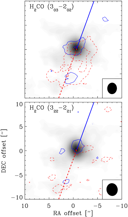
Figure 7: OVRO interferometer maps of H₂CO emission (contours) overlayed on the 1.37 mm continuum emission (greyscale) for L1448–C. The H₂CO emission has been separated into a red (dashed lines) and a blue (solid lines) part (see text for details). Contours start at at 0.2 Jy beam^-1 km s^-1 (2$\sigma$) and each succesive contour is a multiple of this value. Also indicated are the directions of the large scale CO outflow.

The emission from the two unresolved components is estimated to contribute $\sim$25% (1.8 Jy) to the total flux at 1.37 mm. In Fig. 6 flux estimates for the compact components around MM1 and MM2 are compared to those at cm to mm wavelengths (Wootten 1989; Estalella et al. 1991; Mundy et al. 1992; Looney et al. 2000). The emission from MM2 is well fitted over the entire region using a spectral index of $2.35\pm 0.06$, consistent with thermal emission from an optically thick disk. For MM1 a combination of two power laws provides the best fit. At shorter wavelengths a spectral index of $2.44\pm 0.16$ is observed, presumably thermal disk emission. At longer wavelengths a much lower index of $0.15\pm 0.15$ is found consistent with free-free emission from an ionized stellar wind or jet. MM1 is indeed thought to be the source driving the large scale outflow associated with IRAS 16293–2422. In comparison no active outflow is known for MM2. However, it has been suggested that MM2 is responsible for a fossilised flow in the E–W direction $\approx$10$\arcsec$ north of MM1 (see Stark et al. 2004, and references therein).

Gaussian fits to the sizes of these disks in the ($u,v$) plane provide upper limits of $\approx$250 AU in diameter for MM1 and MM2. Using Eq. 1 in the optically thin limit gives estimates of the disk masses for MM1 and MM2 of $0.09-0.24$ M_⊙ and $0.12-0.33$ M_⊙, respectively, again assuming the characteristic dust temperature to be $100-40$ K. Since the spectral indices indicate that the emission is optically thick in both cases, these masses should be treated as lower limits.

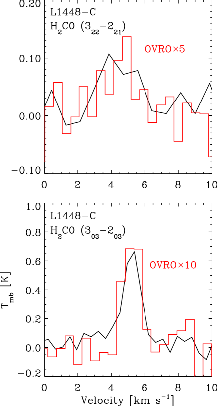
Figure 8: Comparison between the H₂CO line emission towards L1448–C, at the source position, from JCMT single-dish observations (line diagram) and OVRO interferometric observations (histogram) restored with the JCMT beam (22″). The OVRO spectrum has been scaled in order to account for the flux seen in the JCMT spectrum.

4 H₂CO emission: morphology and abundance structure

4.1 L1448–C

The maps of the H₂CO $3_{03}\rightarrow 2_{02}$ and $3_{22}\rightarrow 2_{21}$ emission toward L1448–C are shown in Fig. 7, separated into blue ($4-5$ km s^-1) and red ($5-6$ km s^-1) components. The $3_{03}\rightarrow 2_{02}$ emission appears to be slightly resolved with an extension to the south along the direction of the outflow. The H₂CO $3_{22}\rightarrow 2_{21}$ is detected only at the source position. The velocity structure hints that the emission is related to the known large scale outflow, although the velocities are significantly lower than the high velocity (typically $30-60$ km s^-1) outflow seen in CO and SiO.

As for the continuum data, care has to be taken when interpreting the line interferometer maps due to the low sensitivity to weak large scale emission. A direct comparison between the single-dish spectrum and that obtained from the interferometer observations restored with the single-dish beam is shown in Fig. 8. The interferometer picks up only $\sim 10-20$% of the single-dish flux, suggesting that the extended cold material is resolved out by the interferometer and that a hotter, more compact, component is predominantly picked up. Within the considerable noise and coarsened spectral resolution, the line profiles are consistent with those obtained at the JCMT.

The $3_{22}\rightarrow 2_{21}$/$3_{03}\rightarrow 2_{02}$ line ratio is sensitive to temperature (e.g., van Dishoeck et al. 1993, Mangum & Wootten 1993), especially in the regime of $50-200$ K. For L1448–C, the interferometer data give a ratio of $0.68\pm 0.39$ indicating the presence of hot gas with $T\gtrsim 70$ K. For comparison, the single-dish line ratio is $0.12\pm 0.04$ (Maret et al. 2004), corresponding to $T\approx 20-30$ K. Optical depth effects and abundance variations with radius (i.e., temperature) can affect this ratio, however, so that more detailed radiative transfer modeling is needed for a proper interpretation.

Just as for the continuum data, the analysis of the H₂CO interferometer data requires a detailed model of emission from the more extended envelope as a starting point. Such a model has been presented by Maret et al. (2004) based on multi-line single-dish observations. Those data have been re-analyzed in this work using the Monte Carlo radiative transfer method and molecular data adopted in Schöier et al. (2002). The density and temperature structures are taken from Jørgensen et al. (2002) (see also §3.1) assuming the gas temperature to be coupled to that of the dust. The lines are assumed to be broadened by turbulent motions in addition to thermal line broadening. The adopted value of the turbulent velocity is 0.7 km s^-1 (Jørgensen et al. 2002). Considering only the para-H₂CO data, a good fit ($\chi^{2}_{\mathrm{red}}=0.8$) is obtained using a constant para-H₂CO abundance of $6\times 10^{-10}$ throughout the envelope. A similarly good fit ($\chi^{2}_{\mathrm{red}}=1.0$) can be made to the ortho-H₂CO single-dish data using an abundance of $9\times 10^{-10}$. The uncertainty of these abundance estimates is approximately 20% within the adopted model. The abundance of H₂CO is $\sim$50% larger than that derived for the outer envelope of IRAS 16293–2422 (Schöier et al. 2002).

As shown by Maret et al. (2004), a different interpretation is possible within the same physical model if the ortho-to-para ratio is forced to be equal to 3 and if a different velocity field is used. If the gas is assumed to be in free-fall toward the 0.5 M_⊙ protostar with only thermal line broadening (i.e., no additional turbulent velocity field), evidence of a huge abundance jump ($>$1000) can be found for L1448–C. The location of this jump is at the 100 K radius of the envelope, where thermal evaporation can take place. For L1448–C, this radius lies at 33 AU or 0$\aas@@fstack{\prime\prime}$15, and the interferometer data can be used to test these two different interpretations.

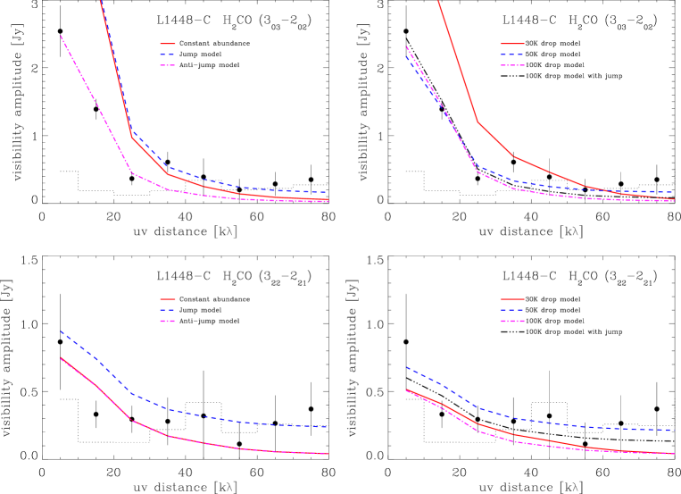
Figure 9: Visibility amplitudes of the observed H₂CO line emission obtained at OVRO toward L1448–C as functions of the projected baseline length. The observations, averaged from 4 to 6 km s^-1 and binned to 10 k$\lambda$, are plotted as filled symbols with 1$\sigma$ error bars. The dotted histogram represents the zero-expectation level. Also shown is the result of applying the same ($u,v$) sampling to the envelope model for various scenarios for the H₂CO abundance distribution. See text for further details.

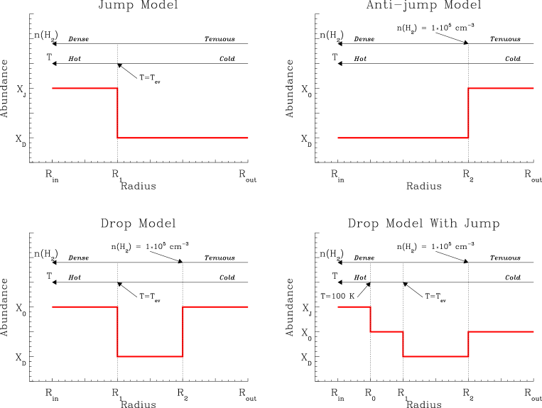
Figure 10: Abundance profiles in various scenarios.

Fig. 9 shows the observed H₂CO visibility amplitudes toward L1448–C. The emission has been averaged over the full extent of the line ($4-6$ km s^-1). Although the signal-to-noise is low, the emission is clearly resolved meaning that hot H₂CO extends to scales larger than $1\arcsec$. Fig. 9 also presents the model predictions assuming a constant para-H₂CO abundance of $6\times 10^{-10}$, consistent with the single-dish data (solid line). The quality of the fit is measured using a $\chi^{2}$ statistic for those visibility amplitudes that are above the zero-expectation limit. From the fit to the observed visibilities in Fig. 9 it is evident that such a constant H₂CO abundance throughout the envelope cannot reproduce the interferometer data ($\chi^{2}_{\mathrm{red}}=26.8$): the $3_{03}-2_{02}$ emission is overproduced on short baselines and underproduced on the longest baselines, while the $3_{22}\rightarrow 2_{21}$/$3_{03}\rightarrow 2_{02}$ model ratio is much lower than the observations.

One possible explanation is that the para-H₂CO abundance drastically increases from $6\times 10^{-10}$ in the outer cool parts of the envelope to $7\times 10^{-7}$ when $T>100$ K, in accordance with the analysis of Maret et al. (2004) and the results for IRAS~16293–2422 (Ceccarelli et al. 2000b; Schöier et al. 2002). This situation is similar to that for the point source needed to explain the continuum emission in §3, since the region where $T>100$ K is only about $0\aas@@fstack{\prime\prime}15$ (33 AU) in radius. Enhancing the abundance in this region will therefore correspond to adding an unresolved point source. The visibility amplitudes for this model are presented in Fig. 9 (dashed line) and agree better with observations on longer baselines than the constant abundance model, but the overall fit is actually slightly worse ($\chi^{2}_{\mathrm{red}}=31.4$). Allowing for a jump at temperatures as low as 50 K cannot be ruled out in the case of IRAS 16293–2422 (Schöier et al. 2002; Doty et al. 2004). This would extend the region of warm material to scales of $1\arcsec$ ($\sim 200$) AU, but this still cannot explain the emission on the shortest baselines, i.e., on scales of $\sim 10-20\arcsec$.

Similarly, the observed emission sampled by the longer baselines could be caused, in part, by H₂CO emission coming from the warm circumstellar disk that was suggested to explain the compact dust emission in §3.1. Here we adopt a disk temperature of 100 K and a corresponding mass (Eq. 1) of 0.016 M_⊙. Further, assuming a diameter of 70 AU, similar to the size of the region where the temperature is higher than 100 K and consistent with the upper limit from observations, the spherically averaged number density of H₂ molecules is $5.3\times 10^{9}$ cm^-3. While the temperature is similar to that found in the inner envelope, the density scale is $\sim 10-50$ times higher. It is found that an H₂CO abundance of $4\times 10^{-9}$ in the disk can explain the observed visibilities on the longer baselines. The abundance in the disk is about 7 times larger than found from single-dish modelling of the envelope alone, but more than an order of magnitude lower than what the thermal evaporation model predicts. The H₂CO abundance in the disk depends critically on the assumed disk properties; e.g., the disk mass used above is only a lower limit and the actual value may be an order of magnitude higher. This would remove the need for a H₂CO abundance jump all together. Still, since the disk is unresolved this does not alleviate the problem of the relatively strong H₂CO $3_{22}\rightarrow 2_{21}$ line emission on the shortest baselines.

In their study of a larger sample of low-mass protostars, Jørgensen et al. (2002) show that CO is significantly depleted in deeply embedded objects such as L1448–C. They also found that intensities of low excitation $J=1\rightarrow 0$ lines are not consistent with constant abundances derived on basis of the higher $J$ lines. Similar trends are seen for other molecular species such as HCO⁺ and HCN by Jørgensen et al. (2004b), who suggest that this is caused by the fact that the time scale for freeze-out of CO and other species is longer than the protostellar lifetime in the outer envelope. This leads to a ‘drop’ abundance profile (see Fig. 10), with CO frozen out in the cold region of the envelope, but with standard or enhanced abundances in the outermost low density cloud and in the inner warmer envelope. The region over which CO is frozen out is determined by the outer radius $R_{2}$ at which the density is high enough that the freeze-out time scale is short compared with the protostellar lifetime and the inner radius $R_{1}$ at which the temperature is low enough that CO does not immediately evaporate from the grain ice mantles. Photodesorption may also play a role in the outermost region. In order for the freeze-out time scale to be shorter than $\sim 10^{4}$ years, the density should be higher than $\sim 10^{5}$ cm^-3.

The H₂CO abundance profile is expected to follow at least partially that of CO, because destruction of gas-phase CO by He⁺ can be a significant source of atomic carbon and oxygen:

$${\rm He}^{+}+{\rm CO}\rightarrow{\rm C}^{+}+{\rm O}+{\rm He}$$ (2)

For the typical densities and temperatures in the outer region, H₂CO is mainly formed through the reaction:

$${\rm CH_{3}}+{\rm O}\rightarrow{\rm H_{2}CO}+{\rm H}$$ (3)

so the H₂CO abundance should drop in regions where CO is frozen out. Indeed, Maret et al. (2004) found a clear correlation between the H₂CO and CO abundances in the outer envelopes where both molecules are depleted, for a sample of eight class 0 protostars. Such an effect would show up in the comparison of interferometer and single-dish data: the interferometer data are mainly sensitive to the $1-10\arcsec$ region of the envelope, where CO is frozen out. The single-dish lines, however, either probe the outer regions of the envelope (low excitation lines), where they quickly become optically thick, or the inner regions (high excitation lines) which are unaffected by the depletion.

In order to test this effect several models in which H₂CO is depleted over roughly the same region as CO were considered (see Fig. 10). Each model was required to simultaneously reproduce all the available multi-transition single-dish data to better than the 3$\sigma$ level. First, an ‘anti-jump’ model was considered where the abundance drops from an initial undepleted value, $X_{0}$, to $X_{\mathrm{D}}$ when the H₂ density is larger than 10⁵ cm^-3. As can be seen in Fig. 9 using $X_{0}=5\times 10^{-9}$ with a drop to $X_{\mathrm{D}}=6\times 10^{-10}$ drastically improves the fit to the observed $3_{03}\rightarrow 2_{02}$ line emission due to opacity effects. The optically thin $3_{22}\rightarrow 2_{21}$ line emission is unaffected by this. The overall fit for this model is good, $\chi^{2}_{\mathrm{red}}=2.0$.

Next, a ‘drop’ H₂CO abundance profile was introduced to simulate the effects of thermal evaporation in the inner warm part of the envelope. First, $T_{\rm ev}$ was taken to be 30 K (see discussion in Jørgensen et al. (2002)), roughly the evaporation temperature of CO. For $T_{\rm ev}=30$ K the jump is located at $R_{1}=7.5\times 10^{15}$ cm ($2\aas@@fstack{\prime\prime}3$). A para-H₂CO abundance of $X_{0}=5\times 10^{-10}$ with a drop to $X_{\mathrm{D}}=3\times 10^{-10}$ in the region of CO depletion provides the lowest $\chi^{2}$ and is consistent with the single-dish data. However, the fit to the interferometer data is not good, $\chi^{2}_{\mathrm{red}}=14.6$. In particular the $3_{03}\rightarrow 2_{02}$ line emission comes out too strong in the model since $X_{0}$ is not allowed to increase enough (constrained by the single-dish data) to become optically thick as in the anti-jump model. The ‘drop’ model does, however, provide a good description of the interferometer emission at both long and short baselines if the H₂CO abundance remains low out to $T\gtrsim 50$ K. For $T_{\rm ev}=50$ K ($R_{1}=1.9\times 10^{15}$ cm; $0\aas@@fstack{\prime\prime}58$), $X_{0}=5\times 10^{-9}$ and $X_{\mathrm{D}}=4\times 10^{-10}$ provides a good fit with $\chi^{2}_{\mathrm{red}}=1.4$. Raising $T_{\rm ev}$ to 100 K ($R_{1}=5.0\times 10^{14}$ cm; $0\aas@@fstack{\prime\prime}15$) provides a slightly worse fit, $\chi^{2}_{\mathrm{red}}=1.8$, for $X_{0}=4\times 10^{-9}$ and $X_{\mathrm{D}}=4\times 10^{-10}$. $X_{0}$ is forced to be in the range $4-5\times 10^{-9}$ from the single dish data, so for $T_{\rm ev}=100$ K less flux is obtained at shorter baselines than compared with the model where $T_{\rm ev}=50$ K because of the smaller emitting volume. Note that these models predict a high $3_{22}\rightarrow 2_{21}$/$3_{03}\rightarrow 2_{02}$ line ratio at large scales where the gas temperature is only $\sim$20 K, due to the fact that the $3_{03}\rightarrow 2_{02}$ line in the outer undepleted region becomes optically thick. On the longest baselines, compact emission from either a disk or an abundance jump would still be consistent with the observations. For example, an additional jump of a factor 10 when $T>100$ K ($R_{0}=R_{1}=5\times 10^{14}$ cm; $X_{\mathrm{D}}=4\times 10^{-10}$; $X_{\mathrm{0}}=4\times 10^{-9}$; $X_{\mathrm{J}}=4\times 10^{-8}$; see Fig. 10) results in an additional $\approx 0.1$ Jy on all baselines and improves the overal fit, $\chi^{2}_{\mathrm{red}}=1.4$, for evaporation at this higher temperature (see Fig. 9). However, since the observed signal is close to the zero-expectation level, no strong conclusions on the presence of this additional jump can be made.

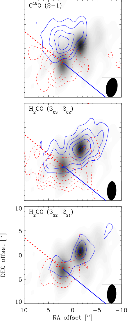
Figure 11: OVRO interferometer maps of IRAS 16293–2422 in C¹⁸O and H₂CO line emission (contours) overlayed on the 1.37 mm continuum emission (greyscale). The molecular line emission has been separated into red (dashed lines) and blue (solid lines) components (see text for details). Contours start at 1.8 Jy beam^-1 km s^-1 for C¹⁸O and at 0.9 Jy beam^-1 km s^-1 for H₂CO. The first contour corresponds to the ’2$\sigma$’-level as estimated from the maps and each successive contour denotes an increase of 2$\sigma$. Also indicated is the direction of the large scale CO outflow.

To summarize: while a constant abundance model can explain the H₂CO emission traced by the single-dish data, it underproduces the emission in the interferometer data on the longest baselines and produces too much $3_{03}-2_{02}$ line emission on the shorter baselines. Adding a compact source of emission either through a hot region of ice mantle evaporation or a circumstellar disk does not provide a better overall fit. A ‘drop’ profile in which the H₂CO abundance largely follows that of CO alleviates these problems, explaining at the same time the emission seen by single-dish and the structure of the emission as traced by the interferometer. The relatively high H₂CO $3_{22}-2_{21}/3_{03}-2_{02}$ ratio at scales of 1 to 10″ is in this scenario caused by a combination of high optical depth of the $3_{03}-2_{02}$ line in the outermost region, and a low H₂CO abundance in the cold dense part of the envelope where CO is frozen out. The best-fit abundances in each of these scenarios are summarized in §5 and compared with those obtained from the similar analysis performed for IRAS 16293–2422 in §4.2.2.

Finally, it should be noted that there may still be other explanations for the high $3_{22}-2_{21}/3_{03}-2_{02}$ line ratio on short baselines. If the H₂CO emission originates from low-velocity entrained material in regions where the outflow interacts with the envelope, the gas temperature may be increased due to weak shocks. Alternatively, the gas temperature can be higher than that of the dust due to heating by ultraviolet or X-ray photons from the protostar which can escape through the biconical outflow cavity and scatter back into the envelope at larger distances (cf. Spaans et al. 1995). Detailed quantitative modeling of these scenarios requires a good physical model of the heating mechanisms and a 2-D radiative transfer and model analysis, both of which are beyond the scope of this paper. In either scenario, the general envelope emission described above still has to be added, and may affect the line ratios through opacity effects.

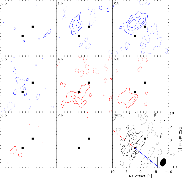
Figure 12: OVRO interferometer maps of C¹⁸O $J=2\rightarrow 1$ line emission (contours) from IRAS 16293–2422. The C¹⁸O emission has been separated into bins of 1 km s¹ and contours are in steps of 0.8 Jy beam^-1 km s^-1 (2$\sigma$). Dotted contours indicate negative values. In the panel with the velocity-integrated line intensity the contours start at 2.0 Jy beam^-1 km s^-1 (2$\sigma$). Also indicated are the positions of the two continuum sources as well as the red- (dashed) and blue-shifted (solid) parts of the large scale outflow.

4.2 IRAS 16293–2422

4.2.1 C¹⁸O emission

The overall C¹⁸O $J=2\rightarrow 1$ line emission for IRAS 16293–2422 obtained at OVRO is presented in Fig. 11, with the channel maps shown in Fig. 12. The emission is clearly resolved and shows a $\sim$6$\arcsec$ separation between the red ($4-7$ km s^-1) and blue ($1-4$ km s^-1) emission peaks. The direction of the red-blue asymmetry is roughly perpendicular to the large scale CO outflow associated with MM1 (Walker et al. 1988, Mizuno et al. 1990, Stark et al. 2004), and may be indicative of overall rotation of the circumbinary material encompassing both MM1 and MM2. The morphology and velocity structure is also consistent with a large ($\sim$1000 AU diameter) rotating gaseous disk around just MM1, however. Such large rotating gaseous disks have been inferred around other sources, including the class I object L1489 (Hogerheijde 2001) and the classical T Tauri star DM Tau (Dutrey et al. 1997), although their C¹⁸O emission is usually too weak to be detected. The C¹⁸O emission clearly avoids the region between the binaries, consistent with the conclusion from the continuum data that this region is void (see §3.2).

In Fig. 13 the interferometer data, restored with a $22\arcsec$ beam, are compared with the JCMT single-dish flux. The interferometer only recovers $\sim$5% of the total single-dish flux, mainly at extreme velocities. The interferometer is not sensitive to the large scale static emission close to the cloud velocity of $\approx$4 km s^-1.

The C¹⁸O data can be used to further test the density structure of the circumbinary envelope. However, as discussed in §4.1 there is now growing evidence that CO is depleted in the cool outer parts of the envelope so that extra care is needed when deducing the density structure from CO observations alone. Schöier et al. (2002) were able to reproduce single-dish CO observations using a constant abundance of about $3\pm 1\times 10^{-5}$ throughout the envelope and with jump models at 20 K, i.e., the characteristic evaporation temperature, $T_{\mathrm{CO}}$, of pure CO ice. Recently, Doty et al. (2004) found that $T_{\mathrm{CO}}\approx 20$ K provided the best fit in their chemical modelling of a large number of molecular species. Here the C¹⁸O $J=2\rightarrow 1$ data are analyzed assuming that the emission originates from 1) a ‘standard’ envelope centered on MM1; and 2) a circumbinary envelope with a cavity centered between the positions of the protostars MM1 and MM2.

Fig. 14 shows the result of applying the ($u,v$) sampling of the observations to the C¹⁸O envelope models. In both the model centered on MM1 and the common envelope model (with a cavity) the observed visibilities are relatively well reproduced using the same constant C¹⁸O abundance of $6\times 10^{-8}$ (solid lines) as obtained from the single-dish analysis, except perhaps at the longest baselines. Note that the density and temperature structures are slightly different for the model with a cavity (see §3.2). Next, thermal evaporation models with a drastic jump at $T_{\mathrm{CO}}=20$ K, as suggested by Doty et al. (2004), were considered. The abundance in the region of depletion, i.e., when $T<20$ K and $n_{\mathrm{H_{2}}}>1\times 10^{5}$ cm^-3, was fixed to $2\times 10^{-8}$, the upper limit obtained by Doty et al. (2004). An undepleted C¹⁸O abundance, $X_{0}$, of $8\times 10^{-8}$ (corresponding to a total CO abundance of about $5\times 10^{-5}$) is found to provide reasonable fits to the observed visibilities in Fig. 14 (dashed lines) as well as CO single-dish data, and is also just consistent with the chemical modelling performed by Doty et al. (2004). This CO abundance is a factor of 2 to 5 lower than typical undepleted abundances. Assuming a still higher evaporation temperature of 50 K brings $X_{0}$ for C¹⁸O up to $2\times 10^{-7}$ (CO up to $1.1\times 10^{-4}$), more in line with what is typically observed in dark clouds. Doty et al. (2004) could not rule out such high evaporation temperatures in their chemical modelling. In all, the success of the envelope model in explaining both the continuum emission as well as the observed CO emission is encouraging and will aid the interpretation of the H₂CO observations.

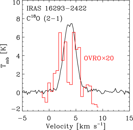
Figure 13: Comparison between the C¹⁸O $J=2\rightarrow 1$ line emission towards IRAS 16293–2422 at the source position, from JCMT single-dish observations (line diagram) and OVRO interferometric observations (histogram) restored with the JCMT beam (22″). The OVRO spectrum has been scaled in order to account for the flux seen in the JCMT spectrum.

The flux detected on the longer baselines provides a limit on the maximum CO abundance in the disk. For a disk around MM1 with diameter 250 AU, temperature 100 K and the mass 0.09 M_⊙ (see §3.2) the spherically averaged H₂ number density is $6.4\times 10^{8}$ cm^-3. It is found that a C¹⁸O abundance of $\approx 2\times 10^{-7}$, corresponding to a total CO abundance of about $1.1\times 10^{-4}$, can account for the emission on the longest baselines. Assuming a lower temperature in the disk of 40 K and the correspondingly higher mass of 0.24 M_⊙ gives almost the same upper limit to the amount of CO in the disk.

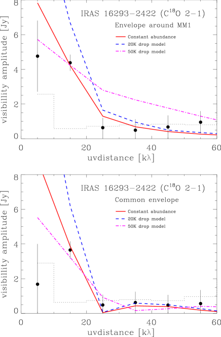
Figure 14: Visibility amplitudes of the observed C¹⁸O $2\rightarrow 1$ line emission obtained at OVRO toward IRAS 16293–2422 as functions of the projected baseline length from the phase center, taken to be at ($2\arcsec,-3\arcsec$) for the envelope around MM1 (top) and ($0\aas@@fstack{\prime\prime}2,-1\aas@@fstack{\prime\prime}2$) for the common envelope (bottom). The observations, averaged over 1 to 7 km s^-1 and binned to 10 k$\lambda$, are plotted as filled symbols with 1$\sigma$ error bars. The dotted histogram represents the zero-expectation level. Also shown is the result of applying the same ($u,v$) sampling to the circumstellar model using a constant C¹⁸O abundance of $6\times 10^{-8}$ (solid lines) for an envelope centered on the protostar MM1 and a common envelope with a cavity. Envelope models where CO is depleted in a region where $n_{\mathrm{H_{2}}}>1\times 10^{5}$ cm^-3 and $T<T_{\mathrm{ev}}$ are also indicated as dashed ($T_{\mathrm{ev}}=20$ K; $X_{0}=8\times 10^{-8}$; $X_{\mathrm{D}}=2\times 10^{-8}$) and dot-dashed ($T_{\mathrm{ev}}=50$ K; $X_{0}=2\times 10^{-7}$; $X_{\mathrm{D}}=2\times 10^{-8}$) lines.

Figure 15: JCMT single-dish spectral maps of the H₂CO emission toward IRAS 16293–2422. The velocity scale is in km s^-1 and the intensity is the main beam brightness temperature in K as indicated in the upper right subplot. The spectral resolution is 0.22 km s^-1. The $3_{22}\rightarrow 2_{21}$ line data have been smoothed to a two times lower spectral resolution.

4.2.2 H₂CO emission

The single-dish observations (see Fig. 15) show that the H₂CO line emission is extended to scales of $\sim$30$\arcsec$. The single-dish $3_{22}\rightarrow 2_{21}$/$3_{03}\rightarrow 2_{02}$ line ratio is $\approx$0.2, suggesting that a cold ($30-40$ K) envelope component dominates the single-dish flux. In contrast, the interferometer $3_{22}\rightarrow 2_{21}$/$3_{03}\rightarrow 2_{02}$ line ratio is $0.69\pm 0.23$ for the red-shifted emission near MM1 and $0.75\pm 0.32$ for the blue-shifted emission close to MM2. This indicates that the temperature is in excess of $\sim 150$ K assuming the density to be at least $10^{6}$ cm^-3. However, as noted for L1448–C, optical depth effects and abundance gradients can affect this ratio.

The velocity channel maps of the H₂CO $3_{03}\rightarrow 2_{02}$ interferometer line emission obtained at OVRO are shown in Fig. 16 for IRAS 16293–2422, whereas the total H₂CO $3_{22}\rightarrow 2_{21}$ and $3_{03}\rightarrow 2_{02}$ maps are included in Fig. 11. The emission is clearly resolved and shows a $\sim$6$\arcsec$ separation between the red ($4-7$ km s^-1) and blue ($1-4$ km s^-1) emission peaks. The direction of the red-blue asymmetry is again roughly perpendicular to the large scale CO outflow associated with MM1, but in contrast with the C¹⁸O OVRO maps, no blue-shifted emission close to MM1 is observed. Instead, the strongest blue-shifted emission occurs close ($<$1$\arcsec$) to MM2. The red-shifted H₂CO emission is found to the south of MM1, but again peaks closer to MM1 than the C¹⁸O emission does.

As for C¹⁸O, only a small fraction ($\sim 5-20$%) of the single-dish flux is recovered by the interferometer (see Fig. 17). The shapes of the H₂CO $3_{03}\rightarrow 2_{02}$ and $3_{22}\rightarrow 2_{21}$ lines are very similar to that of C¹⁸O $J=2\rightarrow 1$ (see Fig. 13), when the interferometer data are restored with the JCMT beam.

The H₂CO emission is interpreted in terms of a common envelope scenario using the cavity model that was seen to best reproduce the emission in §3.2. Alternative models with the envelope centered on MM1 or MM2 have been considered as well, but lead to the same overall conclusions. H₂CO models with and without any abundance jumps or drops are produced for this physical model, following the analysis performed for L1448–C (see Fig. 10). Applying the ($u,v$) sampling from the observations to these models produces visibility amplitudes that are compared with observations in Fig. 18.

Using a constant para-H₂CO abundance of $5\times 10^{-10}$ derived from the single-dish modelling performed in Schöier et al. (2002) produces too much flux on the shorter baselines for both the $3_{03}\rightarrow 2_{02}$ and $3_{22}\rightarrow 2_{21}$ transitions. For IRAS 16293–2422, an abundance jump in the inner hot core due to evaporation of ice mantles is well established from multi-transition single-dish modelling (van Dishoeck et al. 1995; Ceccarelli et al. 2000b; Schöier et al. 2002). Schöier et al. (2002) constrain the location of the jump to $\gtrsim 40$ K, with a jump in abundance of one to three orders of magnitude depending on the adopted evaporation temperature. It is found that a jump model with $T_{\mathrm{ev}}=50$ K (at $R_{1}=6.2\times 10^{15}$ cm = 410 AU = $2\aas@@fstack{\prime\prime}6$) improves the fit to the data ($\chi^{2}_{\mathrm{red}}=7.1$) using $X_{0}=1\times 10^{-10}$ and $X_{\mathrm{J}}=3\times 10^{-9}$ (Fig. 18, left panels). However, this model still produces too much $3_{03}\rightarrow 2_{02}$ line emission on the shortest baselines. This is similar to L1448–C where a better fit was obtained by letting the abundance increase again in the outer region when $n_{\mathrm{H_{2}}}<1\times 10^{5}$ cm^-3 to provide significant optical depth in the $3_{03}\rightarrow 2_{02}$ transition. Such an anti-jump model with $X_{\mathrm{D}}=1\times 10^{-10}$ and $X_{0}=3\times 10^{-9}$ also improves the fit ($\chi^{2}_{\mathrm{red}}=3.6$) in the case of IRAS 16293–2422.

In the drop models two different evaporation temperatures are considered: $T_{\mathrm{ev}}=50$ K and 30 K (at $R_{1}=1.1\times 10^{16}$ cm = 740 AU = $4\aas@@fstack{\prime\prime}6$). As shown in Fig. 18 (right panels) the 30 K model does not provide a good fit to the data ($\chi^{2}_{\mathrm{red}}=17.5$). Using $T_{\mathrm{ev}}=50$ K instead allows $X_{0}$ to be higher and a near-perfect fit ($\chi^{2}_{\mathrm{red}}=0.4$) can be found to both the $3_{03}\rightarrow 2_{02}$ and $3_{22}\rightarrow 2_{21}$ line emission. In this case $X_{\mathrm{D}}=1\times 10^{-10}$ and $X_{0}=4\times 10^{-9}$, i.e., the jump is of a factor 40. A similar jump at 50 K was found by Ceccarelli et al. (2001) from their analysis of the H$2$CO single-dish data. The best-fit abundances in each of these scenarios are summarized in §5 and compared with those obtained from the similar analysis performed for L1448–C in §4.1.

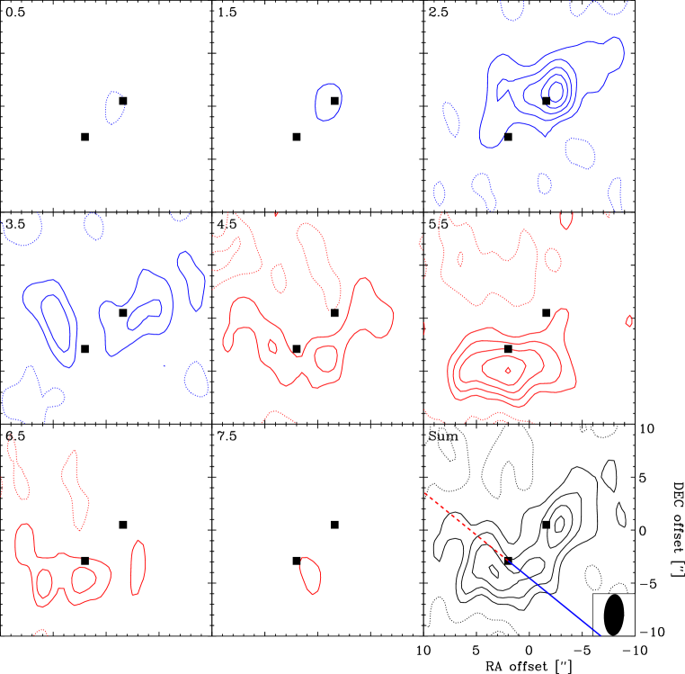
Figure 16: OVRO interferometer maps of H₂CO $3_{03}\rightarrow 2_{02}$ line emission (contours) for IRAS 16293–2422. The H₂CO emission has been separated into bins of 1 km s¹ and contours are in steps of 0.4 Jy beam^-1 km s^-1 (2$\sigma$). In the panel with the velocity-integrated line intensity the contours start at 1.0 Jy beam^-1 km s^-1 (2$\sigma$). Also indicated are the positions of the two continuum sources as well as the red- (dashed) and blue-shifted (solid) parts of the outflow.

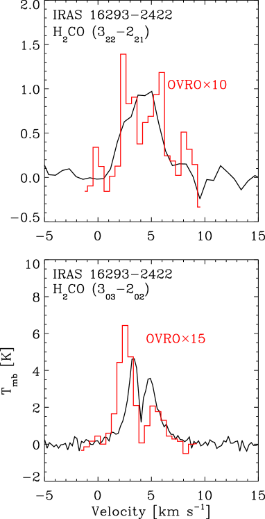
Figure 17: Comparison between the H₂CO line emission towards IRAS 16293–2422 at the source position, from JCMT single-dish observations (line diagram) and OVRO interferometric observations (histogram) restored with the JCMT beam (22″). The OVRO spectrum has been scaled in order to account for the flux seen in the JCMT spectrum.

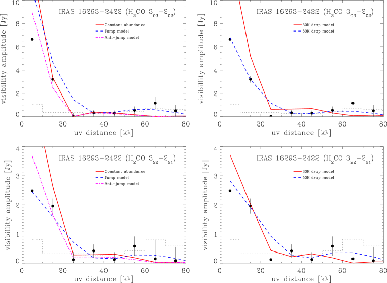
Figure 18: Visibility amplitudes of the observed H₂CO line emission obtained at OVRO toward IRAS 16293–2422 as functions of the projected baseline length from the phase center, taken to be at ($0\aas@@fstack{\prime\prime}2,-1\aas@@fstack{\prime\prime}2$) for the common envelope. The observations, averaged over 1 to 7 km s^-1 and binned to 10 k$\lambda$, are plotted as filled symbols with 1$\sigma$ error bars. The dotted histogram represents the zero-expectation level. Also shown are the results of applying the same ($u,v$) sampling to the circumbinary envelope model using various H₂CO abundance distributions. All models are consistent with available multi-transition single-dish data to within 3$\sigma$. See text and Fig. 10 for details on these models.

The observed flux at the longest baselines gives an upper limit to the para-H₂CO abundance in a disk around MM1. Using the properties of the disk as in §4.2.1 an abundance of $1\times 10^{-9}$ is found to produce about 0.5 Jy on all baselines. For the $\approx$30% more massive disk around MM2 a slightly lower value for the para-H₂CO abundance is found.

Given the complexity of the H₂CO emitting region on small scales ($\lesssim$10$\arcsec$) the envelope model presented in Schöier et al. (2002) is not adequate to fully describe the morphology of the emission observed by the interferometer. Here we simply note that the envelope model can explain the observed flux if jumps in abundance are introduced. The fact that both the H₂CO and C¹⁸O observations can be well reproduced by the common envelope model with a cavity further supports the finding from the continuum observations that little material seems to be located at inter-binary scales.

Table 2: Best fit H₂CO envelope models^a.

Model		L1448–C					IRAS 16293–2422
		$X_{\mathrm{D}}$	$X_{0}$	$X_{\mathrm{J}}$	$\chi^{2}_{\mathrm{red}}$b		$X_{\mathrm{D}}$	$X_{0}$	$X_{\mathrm{J}}$	$\chi^{2}_{\mathrm{red}}$b
Constant abundance		$6\times 10^{-10}$	—	—	26.8		$5\times 10^{-10}$	—	—	11.0
Jump modelc		$6\times 10^{-10}$	—	$6\times 10^{-07}$	31.4		$1\times 10^{-10}$	—	$3\times 10^{-09}$	07.1
Anti-jump model		$6\times 10^{-10}$	$5\times 10^{-09}$	—	02.0		$3\times 10^{-10}$	$4\times 10^{-09}$	—	03.6
30 K drop model		$3\times 10^{-10}$	$5\times 10^{-10}$	—	14.6		$2\times 10^{-10}$	$4\times 10^{-10}$	—	17.5
50 K drop model		$4\times 10^{-10}$	$5\times 10^{-09}$	—	01.4		$1\times 10^{-10}$	$4\times 10^{-09}$	—	00.4
100 K drop model		$4\times 10^{-10}$	$4\times 10^{-09}$	—	01.8		—	—	—	—
100 K drop model with jump		$4\times 10^{-10}$	$4\times 10^{-09}$	$4\times 10^{-08}$	01.4		—	—	—	—

^a All abundances refer to para-H₂CO only.
^b Reduced $\chi^{2}$ from interferometer data. All models are consistent with available single-dish data to within the 3$\sigma$ level.
^c Jump at 100 K for L1448–C and 50 K for IRAS 16293–2422.

5 Origin of the H₂CO emission

Here the results from the previous sections are summarized. Various competing scenarios on the origin of the observed H₂CO emission are discussed and predictions for future generation telescopes are presented, illustrating their potential to distinguish competing scenarios.

5.1 Envelope and/or outflow emission?

In §4 the physical envelope models derived from single-dish observations, and tested against interferometric continuum observations in §3, have used as a basis for interpreting the observed H₂CO emission. The results are summarized in Table 2. It is found that for both IRAS 16293–2422 and L1448–C, the best fit to the H₂CO interferometric observations is obtained with a ‘drop’ abundance profile, in which the H₂CO abundance is lower by more than an order of magnitude in the cold dense zone of the envelope but is high in the inner- and outermost regions. The outer radius of this ‘drop’-zone is set by the distance at which the density drops below $10^{5}$ cm^-3; the inner radius by the distance at which the temperature is above the evaporation temperature $T_{\rm ev}$. Indeed, such a ‘drop’ model with $T_{\rm ev}$=50 K gives very good $\chi^{2}$ fits and reproduces both the single-dish and interferometer data. The fact that two lines of the same molecule with different optical depths were observed simultaneously with OVRO was essential to reach this conclusion. The presence of abundance enhancements in regions where $T\gtrsim 50$ K is consistent with the detailed analysis of multi-transition single-dish H₂CO observations, although the actual values derived here are somewhat different. Interestingly, the inferred abundances $X_{D}$ and $X_{0}$ for the best-fit 50 K drop models are comparable for the two sources. The presence of additional jumps with $X_{J}>X_{0}$ in the innermost hot core region or disk cannot be established with the current data, but requires interferometer observations of higher excitation lines (see §5.4).

Can some of the enhanced H₂CO originate in the outflow? The red-blue asymmetry observed for L1448–C is consistent with the high velocity outflow seen in CO and SiO, but the velocities seen for H₂CO are significantly lower. One explanation is that the emission originates in the acceleration region of the outflow, estimated to be within $2\arcsec$ radius from the star (Guilloteau et al. 1992). An alternative, more plausible scenario is that if H₂CO is associated with the outflow, but located in low-velocity entrained material in regions where the outflow interacts with the envelope, since the red-shifted emission appears to be extended to scales much larger than 2^′′. This would be similar to the case of HCO⁺ (Guilloteau et al. 1992).

For IRAS 16293–2422 the morphology indicates emission in a rotating envelope perpendicular to the direction of the (large-scale) outflow. However, the complicated physical structure of this protobinary object on small spatial scales is not well represented by our spherically symmetric model, so it is not possible to rule out a scenario where some of the emission originates on larger scales due to interaction with the outflow.

To quantify the role of outflows in producing H₂CO abundance enhancements and liberating ice mantles, H₂CO interferometer data at $\sim$1^′′ resolution for a larger sample of sources are needed to investigate whether the velocity pattern is systematically oriented along the outflow axis as in L1448–C. Also, higher sensitivity could reveal whether the profiles have more extended line wings.

5.2 Photon heating of the envelope?

The current models assume that the gas temperature equals the dust temperature. Detailed models of the heating and cooling balance of the gas have indicated that this is generally a good assumption within a spherically symmetric model (Ceccarelli et al. 1996; Doty & Neufeld 1997). However, if the gas temperature were higher than the dust temperature in certain regions, this would be an alternative explanation for the increased $3_{22}-2_{21}$/$3_{03}-2_{02}$ ratio in the interferometer data on short baselines. One possibility discussed in §4.1 would be gas heating by ultraviolet (UV)- or X-ray photons which impact the inner envelope and can escape through the biconical cavity excavated by the outflow. If such photons scatter back into the envelope, they can raise the gas temperature to values significantly in excess of the dust temperature in part of the outer envelope (e.g., Spaans et al. 1995). For IRAS 16293–2422, such photons can further escape through the circumbinary cavity, so that the photons from e.g., MM2 can influence the inner envelope rim around MM1. Since this model would affect the excitation of all molecules present in this gas, not only H₂CO, it can be tested with future multi-line interferometer data of other species. Moreover, the presence of UV photons would have chemical consequences producing enhanced abundances of species like CN in the UV-affected regions, which should be observable. Note that in this scenario, the general colder envelope still has to be added, which, as noted above, can affect the line ratios.

5.3 Disk emission?

The detailed modelling of the continuum emission performed in §3 reveals that there is compact emission in both IRAS 16293–2422 and L1448–C that cannot be explained by the envelope model. The most likely interpretation is that of accretion disks. For L1448–C, where the inner region appears to be less complex, it is found that the observed compact H₂CO emission can be equally well explained originating from a disk as from the inner hot core. However, the need for a drastic jump in abundance depends critically on the properties of the disk. An upper limit on the para-H₂CO abundance in the disk of $\sim$4$\times 10^{-9}$ is derived adopting a temperature of 100 K, a mass of 0.016 M_⊙ and a size of 70 AU and assuming that all the flux on long baselines arises is due to the disk. For IRAS 16293–2422 an upper limit of the abundance in the MM1 disk of $\sim$1$\times 10^{-9}$ is obtained using a mass of 0.09 M_⊙ and a size of 250 AU. A slightly lower upper limit is obtained for MM2 using a disk mass of 0.12 M_⊙. Moreover, the difference between the morphology of the C¹⁸O and H₂CO emission seems to indicate that at least the disk around MM1 contains little H₂CO, even though CO may be nearly undepleted. Note that geometrical effects, for example from the disk potentially shielding parts of the envelope, can cause differences in the appearance between MM1 and MM2.

H₂CO has been detected in protoplanetary disks of T Tauri stars (Dutrey et al. 1997; Aikawa et al. 2003), where confusion due to an envelope or outflow is negligible. Thi et al. (2004) find an integrated H₂CO $3_{03}\rightarrow 2_{02}$ line intensity of 0.14 K km s^-1 (about 1.3 Jy km s^-1) for the T Tauri (class II) star LkCa 15 using the IRAM 30 m telescope. The beam-averaged ($10\aas@@fstack{\prime\prime}8$) H₂CO abundance is about $4\times 10^{-11}$. The OVRO data for IRAS 16293–2422 presented here give a factor of about 50 stronger emission. For L1448–C the emission is about a factor of 10 stronger after correcting for the distance. Thus, if the compact H₂CO emission were coming from disks, they would have to be ‘hotter’ or have higher abundances than in the class II phase. Accretion shocks in the early stages could be responsible for such increased disk temperatures. High-angular resolution ($<1^{\prime\prime}$) data on the velocity structure of the H₂CO lines are needed to distinguish the disk emission from that of the inner envelope.

Table 3: Predicted H₂CO line intensities for L1448–C

Transition	Frequency	$E_{\mathrm{u}}$a		Envelopeb				Envelope w. jumpc				Envelope w. dropd				Envelope+diske
	[GHz]	[K]		[K km s-1]				[K km s-1]				[K km s-1]				[K km s-1]
				$0\aas@@fstack{\prime\prime}3$	$3\arcsec$	$15\arcsec$		$0\aas@@fstack{\prime\prime}3$	$3\arcsec$	$15\arcsec$		$0\aas@@fstack{\prime\prime}3$	$3\arcsec$	$15\arcsec$		$0\aas@@fstack{\prime\prime}3$	$3\arcsec$	$15\arcsec$
$3_{03}\rightarrow 2_{02}$	218.22	21		20	10	2.7		96	11.5	2.7		34	6.6	2.2		137	12	2.7
$3_{22}\rightarrow 2_{21}$	218.48	68		7.2	1.8	0.23		109	3.1	0.27		37	2.8	0.22		160	3.8	0.30
$5_{05}\rightarrow 4_{04}$	362.74	52		31	7.3	0.64		135	8.7	0.69		99	9.9	0.66		180	9.4	0.72
$5_{24}\rightarrow 4_{23}$	363.95	100		16	1.9	0.12		134	3.5	0.18		76	4.5	0.21		183	4.3	0.21
$5_{42/41}\rightarrow 4_{41/40}$	364.10	241		2.4	0.08	0.004		164	2.1	0.08		20	0.62	0.02		268	3.7	0.15

^a Energy of the upper energy level involved in the transition.
^b Constant para-H₂CO abundance of $6\times 10^{-10}$ throughout the envelope.
^c A jump in abundance of a factor 250, from $6\times 10^{-10}$, when $T>100$ K .
^d H₂CO is depleted by about an order of magnitude over roughly the same region as CO ($T_{\mathrm{ev}}=50$ K; $X_{\mathrm{0}}=5\times 10^{-9}$; $X_{\mathrm{D}}=4.0\times 10^{-10}$)
^e H₂CO abundance in the disk is 25 times higher than that in the envelope of $6\times 10^{-10}$.

5.4 Predictions for future generation telescopes

In Table 3, the predicted H₂CO line intensities, integrated over the full extent of the line, are presented for L1448–C using: 1) the envelope model with a constant abundance of $6\times 10^{-10}$, 2) introducing a jump when $T>100$ K ($X_{\mathrm{J}}=1.5\times 10^{-7}$; $X_{\mathrm{D}}=6\times 10^{-10}$), 3) a ‘drop’ abundance profile where H₂CO is depleted over the same region as CO ($T_{\mathrm{ev}}=50$ K; $X_{\mathrm{0}}=5\times 10^{-9}$; $X_{\mathrm{D}}=4\times 10^{-10}$); and 4) the envelope + disk model ($X_{\mathrm{D}}=6\times 10^{-10}$ and disk parameters from §4.1). Beamsizes of $0\aas@@fstack{\prime\prime}3$ and $3\arcsec$ were assumed to characterize the typical spatial resolutions of current and future interferometers. The corresponding intensities picked up by a single-dish beam of $15\arcsec$ are shown for comparison. Using single-dish data alone, it will be difficult to discriminate between these competing scenarios unless the highest frequency lines are obtained. Current interferometers such as OVRO working in the 1 mm window can however constrain some characteristics of the abundance variations in the envelopes, such as the presence of a drop abundance profile. This seems to be the case for the two sources studied here, IRAS 16293–2422 and L1448–C.

Finally, it is clear that observations at 0.^′′3 will have the potential to further discriminate a hot core scenario from that of a warm disk. Indeed, the much improved resolution and sensitivity of next generation interferometers such as CARMA, (e)-SMA, (upgraded) IRAM and ALMA will greatly aid in distinguishing between the competing scenarios discussed above. They will also provide additional constraints on the morphology and velocity structure of the gas on larger and smaller scales. In addition to searching for outflow motions, it is of considerable interest to determine if the hot core gas shows any evidence of infall motions toward the cental source(s). If chemically processed material such as H₂CO and other organics is in a state of infall toward the central protostars it will likely be incorporated in the growing protoplanetary disk and become part of the material from which planetary bodies are formed. With the present data, it is not possible too uniquely separate infall motions from those of rotation and/or outflow.

6 Conclusions

A detailed analysis of the small scale structure of the two low-mass protostars IRAS 16293–2422 and L1448–C has been carried out. Interferometric continuum observations indicate that the inner part of the circumbinary envelope around IRAS 16293–2422 is relatively void of material on scales smaller than the binary separation ($\sim$5$\arcsec$). This implies that the clearing occurs at an early stage of binary evolution and that IRAS 16293–2422 may well develop into a GG Tau-like object in the future. The bulk of the observed emission for both sources is well described using model envelope parameters constrained from single-dish observations, together with unresolved point source emission, presumably due to circumstellar disk(s).

Simultaneous H₂CO line observations indicate the presence of hot and dense gas close to the peak positions of the continuum emission. For both IRAS 16293–2422 and L1448–C, the observed emission cannot be reproduced with a constant abundance throughout the envelope. The H₂CO $3_{22}-2_{21}/3_{03}-2_{02}$ ratio on short baselines ($2-10\arcsec$) is best fit for both sources by an H₂CO ‘drop’ abundance profile in which H₂CO, like CO, is depleted (by more than an order of magnitude) in the cold dense region of the envelope where $T\lesssim 50$ K, but is relatively undepleted in the outermost region where $n_{\mathrm{H_{2}}}<1\times 10^{5}$ cm^-3. In the inner region for $T>50$ K, the abundance jumps back to a high value comparable to that found in the outermost undepleted part. Additional H₂CO abundance jumps —either in the innermost ‘hot core’ region or in the compact circumstellar disk— cannot be firmly established from the current data set.

Based on the morphology and line widths, little of the observed emission toward IRAS 16293–2422 is thought to be directly associated with the known outflow(s). Instead, the emission seems to be tracing gas in a rotating disk perpendicular to the large scale outflow. For L1448–C, the morphology of the H₂CO line emission is consistent with the outflow, but the line widths are significantly smaller and the emission is extended over a large area. Although the above envelope model with a ‘drop’ abundance profile can fit the observations, other scenarios cannot be ruled out. These include the possibility that the outflow (weakly) interacts with the envelope producing regions of enhanced density and temperature in which some H₂CO is liberated and entrained, and a scenario in which part of the envelope gas is heated by UV- or X-ray photons escaping through the outflow cavities.

It is clear that high sensitivity and high spatial resolution observations are critically needed for a better understanding of the chemical and dynamical processes operating during star formation. At the same time, this study also demonstrates that detailed radiative transfer tools are essential for a correct analysis of such data. In the future, the modeling codes need to be extended to multiple dimensions ($>$1D) in order to fully tackle the complex geometry hinted at in current data sets. Predictions for future arrays are provided that illustrate their potential to discriminate between competing scenarios for the origin of the H₂CO abundance enhancements, and presumably that of other complex organics, in low-mass protostars.