Neutrino Processes in Strong Magnetic Fields and Implications for Supernova Dynamics

Abstract

The processes $\nu_{e}+n\rightleftharpoons p+e^{-}$ and $\bar{\nu}_{e}+p\rightleftharpoons n+e^{+}$ provide the dominant mechanisms for heating and cooling the material between the protoneutron star and the stalled shock in a core-collapse supernova. Observations suggest that some neutron stars are born with magnetic fields of at least $\sim 10^{15}$ G while theoretical considerations give an upper limit of $\sim 10^{18}$ G for the protoneutron star magnetic fields. We calculate the rates for the above neutrino processes in strong magnetic fields of $\sim 10^{16}$ G. We find that the main effect of such magnetic fields is to change the equations of state through the phase space of $e^{-}$ and $e^{+}$, which differs from the classical case due to quantization of the motion of $e^{-}$ and $e^{+}$ perpendicular to the magnetic field. As a result, the cooling rate can be greatly reduced by magnetic fields of $\sim 10^{16}$ G for typical conditions below the stalled shock and a nonuniform protoneutron star magnetic field (e.g., a dipole field) can introduce a large angular dependence of the cooling rate. In addition, strong magnetic fields always lead to an angle-dependent heating rate by polarizing the spin of $n$ and $p$. The implications of our results for the neutrino-driven supernova mechanism are discussed.

I Introduction

In this paper we study neutrino processes in strong magnetic fields and their implications for supernova dynamics. Although the detailed mechanism by which massive stars produce supernova explosions is still elusive (see Ref. Bethe (1990) for a review), intense research in the past few decades has led to the following prevalent paradigm. At the exhaustion of nuclear fuels, the Fe core of a massive star collapses. When nuclear density is reached, the inner core bounces and a shock is launched. As the shock propagates outward, it loses energy by dissociating the Fe nuclei falling through it. Eventually, the shock is stalled before exiting the outer core. Meanwhile, the inner core is settling into a protoneutron star by emitting $\nu_{e}$, $\bar{\nu}_{e}$, $\nu_{\mu}$, $\bar{\nu}_{\mu}$, $\nu_{\tau}$, and $\bar{\nu}_{\tau}$. These neutrinos can exchange energy with the material below the stalled shock. The dominant energy-exchange processes are

$$\nu_{e}+n \rightleftharpoons p+e^{-},$$ (1)

$$\bar{\nu}_{e}+p \rightleftharpoons n+e^{+}.$$ (2)

The forward processes in Eqs. (1) and (2) heat the material through absorption of $\nu_{e}$ and $\bar{\nu}_{e}$ while the reverse processes cool the material through capture of $e^{-}$ and $e^{+}$. The competition between heating and cooling of the material by these processes is expected to result in net energy gain for the shock, which then propagates outward again to make a supernova explosion. This is the neutrino-driven supernova mechanism Bethe and Wilson (1985).

Unfortunately, the current consensus is that the neutrino-driven supernova mechanism does not work in spherically symmetric models Rampp and Janka (2000); Liebend rfer et al. (2001). One group has shown that this mechanism works in three-dimensional models where spherical symmetry is broken by convection Fryer and Warren (2002). However, this success has not been confirmed by other groups yet. On the other hand, magnetic fields may be generated during the formation of protoneutron stars and in turn affect supernova dynamics. Magnetic fields of $\sim 10^{12}$ G are commonly inferred for pulsars. Observations also suggest that a number of neutron stars, the so-called magnetars, have magnetic fields of $\sim 10^{15}$ G (see e.g., Refs. Kouveliotou et al. (1999); Gotthelf et al. (1999); Ibrahim et al. (2003)). A theoretical upper limit of $\sim 10^{18}$ G may be estimated for the magnetic fields of new-born neutron stars Lai (2001). While strong magnetic fields may induce supernova explosions directly through dynamic effects such as jet production Khokhlov et al. (1999), and therefore, render the neutrino-driven mechanism irrelevant, the details of this magnetohydrodynamic mechanism have not been worked out or understood yet. In this paper we address the effects of strong magnetic fields on supernova dynamics still in the context of the neutrino-driven mechanism. In particular, we focus on how such fields affect the microscopic processes of heating and cooling the material below the stalled shock.

We describe the neutrino-driven supernova mechanism without magnetic fields in some detail in Sec. II. The rates of the processes in Eqs. (1) and (2) in strong magnetic fields are calculated in Sec. III. The implications of these rates for supernova dynamics are discussed in Sec. IV and conclusions given in Sec. V.

II The Neutrino-Driven Supernova Mechanism

Figure 1: A sketch of the region of interest. The neutrinosphere of radius $R_{\nu}=50$ km effectively defines the surface of the protoneutron star. The stalled shock is at an average radius $R_{s}=200$ km. At the gain radius $R_{g}$, the rate for heating by absorption of $\nu_{e}$ and $\bar{\nu}_{e}$ equals that for cooling by capture of $e^{-}$ and $e^{+}$. Heating dominates cooling above $R_{g}$.

In this section we give a more quantitative description of the neutrino-driven supernova mechanism in the absence of magnetic fields. As this mechanism has not been fully established yet, we will use parameters typical of current models to illustrate the essence of these models rather than focus on the numerical details of a specific model. We are interested in times of $\lesssim 0.5$ s after the core collapse, which correspond to the critical period for the neutrino-driven supernova mechanism. The region of interest is above the protoneutron star but below the stalled shock as illustrated in Fig. 1. We consider that neutrinos are emitted from a neutrinosphere of radius $R_{\nu}=50$ km that effectively defines the surface of the protoneutron star (see e.g., Fig. 11.1 in Ref. Raffelt (1996)). The stalled shock is taken to be at an average radius $R_{s}=200$ km. The material in the region of interest has typical entropies of $\sim 10$ (in units of Boltzmann constant per nucleon) and typical temperatures of several MeV. For these conditions, the material can be characterized as a gas of $n$, $p$, $e^{-}$, $e^{+}$, and $\gamma$ (photons). The predominant cooling processes are the reverse reactions in Eqs. (1) and (2) while the predominant heating processes are the corresponding forward reactions [note that similar charged-current processes involving $\nu_{\mu(\tau)}$ and $\bar{\nu}_{\mu(\tau)}$ are energetically forbidden for the neutrino energies and material conditions available in supernovae]. Cooling dominates heating near the neutrinosphere. However, the cooling rate decreases much more steeply with increasing radius than the heating rate. These two rates becomes equal at the gain radius $R_{g}$, above which heating dominates. Thus, the heating and cooling rates are crucial to a quantitative discussion of the neutrino-driven supernova mechanism. These rates are calculated below.

We start with a description of neutrino emission by the protoneutron star. The $\nu_{e}$ luminosity $L_{\nu_{e}}$ is taken to be the same as the $\bar{\nu}_{e}$ luminosity $L_{\bar{\nu}_{e}}$. We assume $L_{\nu_{e}}=L_{\bar{\nu}_{e}}=4\times 10^{52}$ erg s^-1 during the epoch relevant for shock revival by neutrino heating. As $\nu_{e}$ and $\bar{\nu}_{e}$ are roughly in thermal equilibrium with the matter at the neutrinosphere, their luminosities approximately correspond to those of black-body radiation for a Fermi-Dirac neutrino energy distribution with zero chemical potential:

$$L_{\nu_{e}}=L_{\bar{\nu}_{e}}\sim\frac{7\pi^{3}}{240}[T(R_{\nu})]^{4}R_{\nu}^{2}\sim 4\times 10^{52}\left[\frac{T(R_{\nu})}{4\ \mathrm{MeV}}\right]^{4}\left(\frac{R_{\nu}}{50\ \mathrm{km}}\right)^{2}\ \mathrm{erg\ s}^{-1}.$$ (3)

In the above equation, $T(R_{\nu})$ is the temperature at the neutrinosphere. Throughout this paper, we adopt units where the Planck constant $\hbar$, the speed of light $c$, and the Boltzmann constant $k$ are set to unity.

Due to the difference in the interaction of $\bar{\nu}_{e}$ and $\nu_{e}$ with the protoneutron star matter, their emission is more complicated than implied by the crude estimate in Eq. (3). As there are fewer protons to absorb $\bar{\nu}_{e}$ than neutrons to absorb $\nu_{e}$, $\bar{\nu}_{e}$ decouple from the protoneutron star matter at higher temperature and density than $\nu_{e}$. This results in a higher average energy for $\bar{\nu}_{e}$ (see below). However, due to the steep temperature and density gradients near the protoneutron star surface, the radii for $\bar{\nu}_{e}$ and $\nu_{e}$ decoupling are essentially the same. Detailed neutrino transport calculations show that $\bar{\nu}_{e}$ and $\nu_{e}$ can be considered as having the same luminosity and neutrinosphere but significantly different average energies (see e.g., Ref. Janka (1995)). The normalized $\nu_{e}$ and $\bar{\nu}_{e}$ energy distributions can be described by functions of the form

$$f_{\nu}(E_{\nu})=\frac{1}{F_{2}(\eta_{\nu})T_{\nu}^{3}}\frac{E_{\nu}^{2}}{\exp[(E_{\nu}/T_{\nu})-\eta_{\nu}]+1},$$ (4)

where the subscript $\nu$ refers to $\nu_{e}$ or $\bar{\nu}_{e}$, $E_{\nu}$ is the neutrino energy, $T_{\nu}$ and $\eta_{\nu}$ are two positive parameters, and $F_{2}(\eta_{\nu})$ is a specific case of the general Fermi integral $F_{n}(\eta)$ defined as

$$F_{n}(\eta)\equiv\int_{0}^{\infty}\frac{x^{n}}{\exp(x-\eta)+1}\,\mathrm{d}x.$$ (5)

The parameter $T_{\nu}$ is related to the average neutrino energy $\langle E_{\nu}\rangle$ as

$$\langle E_{\nu}\rangle=\frac{F_{3}(\eta_{\nu})}{F_{2}(\eta_{\nu})}T_{\nu}.$$ (6)

We take $\eta_{\nu_{e}}=\eta_{\bar{\nu}_{e}}=3$, $\langle E_{\nu_{e}}\rangle=11$ MeV, and $\langle E_{\bar{\nu}_{e}}\rangle=16$ MeV. For these parameters, $T_{\nu_{e}}=2.75$ MeV and $T_{\bar{\nu}_{e}}=4$ MeV, which are close to $T(R_{\nu})$ estimated from Eq. (3).

Figure 2: A sketch of the geometry for calculating the differential neutrino number density $\mathrm{d}^{2}n_{\nu}/\mathrm{d}E_{\nu}\mathrm{d}\Omega_{\nu}$ at radius $r$. For a specific radial direction $\bf{\hat{r}}$, the differential solid angle $\mathrm{d}\Omega_{\nu}$ is defined by the polar angle $\theta_{\nu}$ between $\bf{\hat{r}}$ and the direction of the neutrino momentum $\bf{\hat{p}}_{\nu}$ (the corresponding azimuthal angle $\phi_{\nu}$ is not shown). Only neutrinos emitted with $\sqrt{1-(R_{\nu}/r)^{2}}\leq\cos\theta_{\nu}\leq 1$ can contribute to $\mathrm{d}^{2}n_{\nu}/\mathrm{d}E_{\nu}\mathrm{d}\Omega_{\nu}$.

To calculate the rate of heating by neutrino absorption processes, we need the differential neutrino number density per unit energy interval and per unit solid angle $\mathrm{d}^{2}n_{\nu}/\mathrm{d}E_{\nu}\mathrm{d}\Omega_{\nu}$ at radius $r>R_{\nu}$ as measured from the center of the protoneutron star. For a specific radial direction $\mathbf{\hat{r}}$, the differential solid angle $\mathrm{d}\Omega_{\nu}$ is defined by the polar angle $\theta_{\nu}$ between $\mathbf{\hat{r}}$ and the direction of the neutrino momentum $\mathbf{\hat{p}}_{\nu}$ (see Fig. 2) and by the corresponding azimuthal angle $\phi_{\nu}$. We assume that only neutrinos emitted with $\sqrt{1-(R_{\nu}/r)^{2}}\leq\cos\theta_{\nu}\leq 1$ can contribute to $\mathrm{d}^{2}n_{\nu}/\mathrm{d}E_{\nu}\mathrm{d}\Omega_{\nu}$ (see Fig. 2). Thus,

$$\frac{\mathrm{d}^{2}n_{\nu}}{\mathrm{d}E_{\nu}\mathrm{d}\Omega_{\nu}}=\left\{\begin{array}[]{ll}L_{\nu}f_{\nu}(E_{\nu})/(4\pi^{2}R_{\nu}^{2}\langle E_{\nu}\rangle),&\text{for }\sqrt{1-(R_{\nu}/r)^{2}}\leq\cos\theta_{\nu}\leq 1,\\ 0,&\text{otherwise}.\end{array}\right.$$ (7)

The corresponding neutrino occupation number $\tilde{f}_{\nu}(E_{\nu})$ is

$$\tilde{f}_{\nu}(E_{\nu})=\frac{(2\pi)^{3}}{E_{\nu}^{2}}\frac{\mathrm{d}^{2}n_{\nu}}{\mathrm{d}E_{\nu}\mathrm{d}\Omega_{\nu}}.$$ (8)

Note that

$$L_{\nu}=4\pi R_{\nu}^{2}\int_{0}^{2\pi}\mathrm{d}\phi_{\nu}\int_{0}^{1}\cos\theta_{\nu}\,\mathrm{d}\!\cos\theta_{\nu}\int_{0}^{\infty}E_{\nu}\frac{\mathrm{d}^{2}n_{\nu}}{\mathrm{d}E_{\nu}\mathrm{d}\Omega_{\nu}}\,\mathrm{d}E_{\nu},$$ (9)

where $\mathrm{d}^{2}n_{\nu}/\mathrm{d}E_{\nu}\mathrm{d}\Omega_{\nu}$ is evaluated at $r=R_{\nu}$.

To zeroth order in $m_{N}^{-1}$ where $m_{N}$ is the nucleon mass, the cross sections for the forward processes in Eqs. (1) and (2) are

$$\sigma_{\nu N}^{(0)}=\frac{G_{F}^{2}\cos^{2}\theta_{C}}{\pi}(f^{2}+3g^{2})p_{e}E_{e},$$ (10)

where the subscript $\nu N$ refers to $\nu_{e}$ absorption on $n$ or $\bar{\nu}_{e}$ absorption on $p$, $G_{F}=(292.8\ \mathrm{GeV})^{-2}$ is the Fermi constant, $\theta_{C}$ is the Cabbibo angle ($\cos^{2}\theta_{C}=0.95$), $f=1$ and $g=1.26$ are the vector and axial-vector coupling coefficients, respectivley, of the weak interaction, and $p_{e}$ and $E_{e}=\sqrt{p_{e}^{2}+m_{e}^{2}}$ are the momentum and energy, respectively, of the electron or positron in the final state ($m_{e}$ is the electron mass). To the same order in $m_{N}^{-1}$, conservation of momentum and energy gives

$$E_{e}=E_{\nu}\pm\Delta,$$ (11)

where $\Delta=1.293$ MeV is the neutron-proton mass difference, the plus sign is for absorption of $\nu_{e}$, and the minus sign is for absorption of $\bar{\nu}_{e}$. Note that there is a threshold energy of $\Delta+m_{e}$ for $\bar{\nu}_{e}$ absorption on $p$.

At radius $r>R_{\nu}$, the heating rate per nucleon $\dot{q}_{h}^{(0)}$ due to absorption of $\nu_{e}$ and $\bar{\nu}_{e}$ is

$$\dot{q}_{h}^{(0)} = Y_{n}\int\mathrm{d}\Omega_{\nu_{e}}\int_{0}^{\infty}(E_{\nu_{e}}+\Delta)\sigma_{\nu_{e}n}^{(0)}\frac{\mathrm{d}^{2}n_{\nu_{e}}}{\mathrm{d}E_{\nu_{e}}\mathrm{d}\Omega_{\nu_{e}}}\,\mathrm{d}E_{\nu_{e}}$$ (12)

$$+ Y_{p}\int\mathrm{d}\Omega_{\bar{\nu}_{e}}\int_{\Delta+m_{e}}^{\infty}(E_{\bar{\nu}_{e}}-\Delta)\sigma_{\bar{\nu}_{e}p}^{(0)}\frac{\mathrm{d}^{2}n_{\bar{\nu}_{e}}}{\mathrm{d}E_{\bar{\nu}_{e}}\mathrm{d}\Omega_{\bar{\nu}_{e}}}\,\mathrm{d}E_{\bar{\nu}_{e}}$$

$$= (3.83\times 10^{3}Y_{n}+5.32\times 10^{3}Y_{p})\left[1-\sqrt{1-(R_{\nu}/r)^{2}}\right]\ \mathrm{MeV\ s}^{-1}\ \mathrm{nucleon}^{-1},$$

where the numerical coefficients correspond to the parameters $L_{\nu_{e}}$, $L_{\bar{\nu}_{e}}$, $T_{\nu_{e}}$, $T_{\bar{\nu}_{e}}$, $\eta_{\nu_{e}}$, and $\eta_{\bar{\nu}_{e}}$ adopted above, and $Y_{n}$ and $Y_{p}$ are the neutron and proton number fractions, respectively. As the material is neutral, $Y_{n}=1-Y_{e}$ and $Y_{p}=Y_{e}$, where $Y_{e}$ is the net electron number per nucleon. The radial dependence in Eq. (12) comes from the integration over $\mathrm{d}\Omega_{\nu}$ and accounts for the geometric dilution of the neutrino number density. Note that for $r\gg R_{\nu}$, $\dot{q}_{h}^{(0)}\propto r^{-2}$. Taking $Y_{e}=0.5$, we calculate $\dot{q}_{h}^{(0)}$ from Eq. (12) and show the result as the solid curve in Fig. 3.

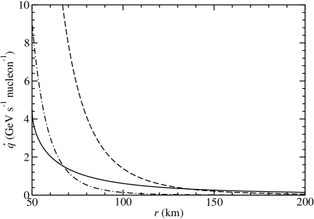
Figure 3: The heating rate per nucleon $\dot{q}_{h}^{(0)}$ (solid curve) and the cooling rate per nucleon $\dot{q}_{c}^{(0)}$ [dashed ($S=10$) and dot-dashed ($S=20$) curves] as functions of radius $r$. The gain radius is at $R_{g}=137$ and 68 km for entropies of $S=10$ and 20, respectively.

Next we calculate the cooling rate due to the reverse processes in Eqs. (1) and (2). It is convenient to define a volume reaction rate, which gives the rate of e.g., $e^{+}$ capture per neutron when multiplied by the $e^{+}$ number density $n_{e^{+}}$. In the absence of magnetic field, the volume reaction rate $\Gamma_{eN}^{(0)}$ is simply $v\sigma_{eN}^{(0)}$, where $v$ is the relative velocity between the reacting particles and $\sigma_{eN}^{(0)}$ is the cross section for $e^{+}$ capture on $n$ or $e^{-}$ capture on $p$. To zeroth order in $m_{N}^{-1}$, the volume reaction rates for these processes are

$$\Gamma_{eN}^{(0)}=\frac{G_{F}^{2}\cos^{2}\theta_{C}}{2\pi}(f^{2}+3g^{2})E_{\nu}^{2}.$$ (13)

In Eq. (13),

$$E_{\nu}=E_{e}\pm\Delta,$$ (14)

where the plus sign is for $e^{+}$ capture on $n$ and the minus sign is for $e^{-}$ capture on $p$. The cooling rate per nucleon $\dot{q}_{c}^{(0)}$ is then

$$\dot{q}_{c}^{(0)}=\frac{Y_{n}}{\pi^{2}}\int_{0}^{\infty}\frac{E_{e^{+}}\Gamma_{e^{+}n}^{(0)}p_{e^{+}}^{2}}{\exp[(E_{e^{+}}/T)+\eta_{e}]+1}\,\mathrm{d}p_{e^{+}}+\frac{Y_{p}}{\pi^{2}}\int_{\sqrt{\Delta^{2}-m_{e}^{2}}}^{\infty}\frac{E_{e^{-}}\Gamma_{e^{-}p}^{(0)}p_{e^{-}}^{2}}{\exp[(E_{e^{-}}/T)-\eta_{e}]+1}\,\mathrm{d}p_{e^{-}},$$ (15)

where $T$ is the temperature, $\eta_{e}$ is the electron degeneracy parameter, and $\sqrt{\Delta^{2}-m_{e}^{2}}$ is the threshold momentum for $e^{-}$ capture on $p$.

To evaluate $\dot{q}_{c}^{(0)}$ we need $T$ and $\eta_{e}$. We take

$$T(r)=T(R_{\nu})\frac{R_{\nu}}{r}=4\left(\frac{50\ \mathrm{km}}{r}\right)\ \mathrm{MeV}$$ (16)

for $R_{\nu}\leq r\leq R_{s}$ (see e.g., Ref. Janka (2001)). We assume that the material in the region of interest can be characterized by a typical electron fraction $Y_{e}$ and a typical entropy per nucleon $S$. We then obtain $\eta_{e}$ together with the matter density $\rho$ from the equations of state:

$$\frac{\rho Y_{e}}{m_{N}} = n_{e^{-}}-n_{e^{+}},$$ (17)

$$S = S_{N}+S_{\gamma}+S_{e^{-}}+S_{e^{+}},$$ (18)

where $S_{N}$, $S_{\gamma}$, $S_{e^{-}}$, and $S_{e^{+}}$ are the contributions to $S$ from nucleons, photons, electrons, and positrons, respectively. The expressions for $n_{e^{-}}$, $n_{e^{+}}$, $S_{N}$, $S_{\gamma}$, $S_{e^{-}}$, and $S_{e^{+}}$ are given in Appendix A. We note that for extremely relativistic $e^{-}$ and $e^{+}$,

$$n_{e^{-}}-n_{e^{+}} = \frac{\eta_{e}}{3}\left(1+\frac{\eta_{e}}{\pi^{2}}\right)T^{3},$$ (19)

$$S_{e^{-}}+S_{e^{+}} = \frac{7\pi^{2}}{45}\left(1+\frac{15\eta_{e}^{2}}{7\pi^{2}}\right)\left(\frac{m_{N}}{\rho}\right)T^{3}.$$ (20)

While we always use the expressions in Appendix A to calculate the results presented in this paper, we find that Eqs. (19) and (20) are excellent approximations to the corresponding general expressions (without magnetic fields) for the conditions in the region of interest.

$\begin{array}[]{@{}c@{\hspace{.2in}}c@{}}\includegraphics*[width=234.87749pt,keepaspectratio]{fig4a.eps}\hfil\hskip 14.45377pt&\includegraphics*[width=234.87749pt,keepaspectratio]{fig4b.eps}\end{array}$

Figure 4: The matter density $\rho$ (a) and the electron degeneracy parameter $\eta_{e}$ (b) as functions of radius $r$. The solid ($S=10$) and dashed ($S=20$) curves are for the case of no magnetic field. The dot-dashed ($S=10$) and dot-dot-dashed ($S=20$) curves are for the case of a uniform magnetic field of $B=10^{16}$ G. The magnetic field greatly reduces $\eta_{e}$ for an entropy of $S=10$. For $S=20$, $\eta_{e}$ is very small even for the case of no magnetic field.

Numerical models Rampp and Janka (2000); Liebend rfer et al. (2001) show that $Y_{e}$ and $S$ tend to rise sharply over a short distance above the neutrinosphere and then stay approximately constant. As cooling always dominates near the neutrinosphere, the gain radius lies in the region where $Y_{e}$ and $S$ can be taken as constant. Thus, we assume no radial dependence for $Y_{e}$ and $S$ in determining the gain radius. Taking $Y_{e}=0.5$ and $S=10$ and 20, we calculate $\rho$ and $\eta_{e}$ as functions of $r$ from Eq. (16) and the equations of state [see Eqs. (17) and (18) and Appendix A]. The results are shown as the solid ($S=10$) and dashed ($S=20$) curves in Fig. 4a for $\rho$ and Fig. 4b for $\eta_{e}$. We also calculate the corresponding $\dot{q}_{c}^{(0)}$ from Eq. (15) and show the results as the dashed ($S=10$) and dot-dashed ($S=20$) curves in Fig. 3 along with the result for $\dot{q}_{h}^{(0)}$ (solid curve). It can be seen that the gain radius is at $R_{g}=137$ and 68 km for $S=10$ and 20, respectively. As the shock is at radius $R_{s}=200$ km, there is a large region for net heating below the shock in both cases. Note that the location of the gain radius is rather sensitive to $S$. A gain radius below the shock ($R_{g}<R_{s}$) exists only for $S\gtrsim 10$. We have also done calculations for different values of $Y_{e}$ and found that the effects of strong magnetic fields to be discussed are qualitatively the same for $Y_{e}\gtrsim 0.3$. For clarity of presentation, we focus on the results for $Y_{e}=0.5$.

In the above calculation of $\dot{q}_{h}^{(0)}$ and $\dot{q}_{c}^{(0)}$, we have ignored Pauli blocking of the final states by the $e^{-}$, $e^{+}$, $\nu_{e}$, and $\bar{\nu}_{e}$ (see e.g., Ref. Gvozdev and Ognev (2002)) in the region above the neutrinosphere. In the case of $\dot{q}_{h}^{(0)}$, the $e^{-}$ and $e^{+}$ produced by $\nu_{e}$ and $\bar{\nu}_{e}$ absorption have typical energies of $\sim 20$ MeV that are much higher than the average energies of $e^{-}$ and $e^{+}$ in the gas. So Pauli blocking is unimportant for calculating $\dot{q}_{c}^{(0)}$, especially in the region near and above the gain radius. In the case of $\dot{q}_{c}^{(0)}$, the neutrino occupation number $\tilde{f}_{\nu}(E_{\nu})$ can be calculated from Eq. (8). For the adopted parameters, we find $\tilde{f}_{\nu_{e}}(E_{\nu_{e}})\leq 0.37$ and $\tilde{f}_{\bar{\nu}_{e}}(E_{\bar{\nu}_{e}})\leq 0.083$ for $\sqrt{1-(R_{\nu}/r)^{2}}\leq\cos\theta_{\nu}\leq 1$ and $\tilde{f}_{\nu_{e}}(E_{\nu_{e}})=\tilde{f}_{\bar{\nu}_{e}}(E_{\bar{\nu}_{e}})=0$ otherwise. As the range of $\cos\theta_{\nu}$ for finite $\tilde{f}_{\nu}(E_{\nu})$ diminishes with increasing $r$, Pauli blocking in this case is also insignificant in the region near and above the gain radius. Thus, ignoring Pauli blocking in the calculation of $\dot{q}_{h}^{(0)}$ and $\dot{q}_{c}^{(0)}$ has little effect on our discussion of the gain radius above. For the same reasons, we will ignore Pauli blocking in the calculation of the heating and cooling rates in strong magnetic fields. This approximation will not affect the comparison of the gain radii for the cases without and with strong magnetic fields.

III Heating and Cooling Rates in Magnetic Fields

In this section we calculate the rates of heating and cooling by the processes in Eqs. (1) and (2) in strong magnetic fields. We consider a uniform magnetic field of constant strength $B$ in the $z$-direction. Observations indicate that neutron stars may have magnetic fields up to $\sim 10^{15}$ G long after their birth in supernovae. This suggests that magnetic fields of at least $\sim 10^{15}$ G can be generated during the formation of some neutron stars. An upper limit of $\sim 10^{18}$ G for protoneutron star magnetic fields can be estimated by equating the magnetic energy to the gravitational binding energy of a neutron star Lai (2001). In this paper we consider protoneutron star magnetic fields of $B\sim 10^{16}$ G.

An obvious effect of the magnetic field is polarization of the spin of a nonrelativistic nucleon due to the interaction Hamiltonian

$$-\bm{\mu}\cdot\mathbf{B}=-\mu\sigma_{z}B.$$ (21)

In Eq. (21), $\bm{\mu}=\mu\bm{\sigma}$ is the nucleon magnetic moment, where $\mu=2.79\mu_{N}$ for $p$ and $\mu=-1.91\mu_{N}$ for $n$ with $\mu_{N}=e/(2m_{p})$ being the nuclear magneton, and $\bm{\sigma}$ refers to the Pauli spin matrices. For a nucleon gas of temperature $T$, the net polarization $\chi$ is

$$\chi=\frac{\exp(\mu B/T)-\exp(-\mu B/T)}{\exp(\mu B/T)+\exp(-\mu B/T)}.$$ (22)

For $|\mu B/T|\ll 1$, Eq. (22) reduces to

$$\chi=\frac{\mu B}{T}=3.15\times 10^{-2}\left(\frac{\mu}{\mu_{N}}\right)\left(\frac{B}{10^{16}\ \mathrm{G}}\right)\left(\frac{\mathrm{MeV}}{T}\right).$$ (23)

In addition, the motion of a proton in the $xy$-plane perpendicular to the magnetic field is quantized into Landau levels (see e.g. Ref. Landau and Lifshitz (1977)) with energies

$$E(n_{L},\,k_{pz})=\frac{k_{pz}^{2}}{2m_{p}}+\left(n_{L}+\frac{1}{2}\right)\frac{eB}{m_{p}},\ n_{L}=0,\ 1,\ 2,\ \cdots,$$ (24)

where $k_{pz}$ is the proton momentum in the $z$-direction. As $eB/m_{p}=63(B/10^{16}\ \mathrm{G})$ keV, a proton in a gas of temperature $T\gtrsim 1$ MeV can occupy Landau levels with $n_{L}\gg 1$ for $B\sim 10^{16}$ G. From the correspondence principle, the proton motion in this case can be considered as classical. Thus, we only need to take into account polarization of the spin by the magnetic field for both $p$ and $n$.

For the conditions of interest here, $e^{-}$ and $e^{+}$ are relativistic. Their Landau levels Johnson and Lippmann (1949) have energies

$$E_{e}(n,\,p_{ez})=\sqrt{p_{ez}^{2}+m_{e}^{2}+2neB},\ n=0,\ 1,\ 2,\ \cdots,$$ (25)

where $p_{ez}$ is the momentum of $e^{-}$ or $e^{+}$ in the $z$-direction. The result in Eq. (25) takes spin into account. Note that the Landau levels of $e^{-}$ and $e^{+}$ have degeneracy $g_{n}=1$ (corresponding to a single spin state) for the $n=0$ state but $g_{n}=2$ (corresponding to two spin states) for all $n>0$ states. For a given $E_{e}$, the maximum value $n_{\mathrm{max}}$ of $n$ is

$$n_{\mathrm{max}}=\left[\frac{E_{e}^{2}-m_{e}^{2}}{2eB}\right]_{\mathrm{int}}=\left[8.45\times 10^{-3}\left(\frac{E_{e}^{2}-m_{e}^{2}}{\mathrm{MeV}^{2}}\right)\left(\frac{10^{16}\ \mathrm{G}}{B}\right)\right]_{\mathrm{int}},$$ (26)

where [ ]_int denotes the integer part of the argument. Thus, $e^{-}$ and $e^{+}$ with $E_{e}\lesssim 10$ MeV can only occupy the Landau level with $n=0$ in magnetic fields of $B\sim 10^{16}$ G. The phase space of $e^{-}$ and $e^{+}$ in this case is dramatically affected by magnetic fields. In general, the integration over the phase space is changed from the classical case to the case of Landau levels according to

$$\frac{1}{4\pi^{3}}\int\mathrm{d}\Omega\int p_{e}^{2}\,\mathrm{d}p_{e}\to\frac{eB}{2\pi^{2}}\sum_{n=0}^{n_{\mathrm{max}}}g_{n}\int\mathrm{d}p_{ez},$$ (27)

where $\Omega$ is the solid angle in the classical momentum space and $p_{ez}$ is restricted to positive values.

III.1 Heating Rate in Magnetic Fields

We first calculate the heating rate due to the forward processes in Eqs. (1) and (2) in magnetic fields. As we only consider magnetic fields of $B\sim 10^{16}$ G, the energy scale $\sqrt{eB}=7.69(B/10^{16}\ \mathrm{G})^{1/2}$ MeV is much lower than the mass of the $W$ (80 GeV) or $Z$ boson (91 GeV). Thus, the weak interaction is unaffected by such magnetic fields. However, such strong magnetic fields can change the cross sections for the forward processes in Eqs. (1) and (2) by polarizing the spin of $n$ and $p$ in the initial state and by changing the phase space of the $e^{-}$ and $e^{+}$ in the final state. The new cross sections to zeroth order in $m_{N}^{-1}$ are derived in Appendix B using the Landau wavefunctions of $e^{-}$ and $e^{+}$. The results are

$$\sigma_{\nu N}(B)=\sigma_{B}^{(1)}\left[1+2\chi\frac{(f\pm g)g}{f^{2}+3g^{2}}\cos\Theta_{\nu}\right]+\sigma_{B}^{(2)}\left[\frac{f^{2}-g^{2}}{f^{2}+3g^{2}}\cos\Theta_{\nu}+2\chi\frac{(f\mp g)g}{f^{2}+3g^{2}}\right],$$ (28)

where we have factored out two energy-dependent terms

$$\sigma_{B}^{(1)} = \frac{G_{F}^{2}\cos^{2}\theta_{C}}{2\pi}(f^{2}+3g^{2})eB\sum_{n=0}^{n_{\mathrm{max}}}\frac{g_{n}E_{e}}{\sqrt{E_{e}^{2}-m_{e}^{2}-2neB}},$$ (29)

$$\sigma_{B}^{(2)} = \frac{G_{F}^{2}\cos^{2}\theta_{C}}{2\pi}(f^{2}+3g^{2})eB\frac{E_{e}}{\sqrt{E_{e}^{2}-m_{e}^{2}}}.$$ (30)

In Eq. (28), $\Theta_{\nu}$ is the angle between the neutrino momentum and the magnetic field, the upper sign is for $\nu_{e}$ absoprtion on $n$, and the lower sign is for $\bar{\nu}_{e}$ absoprtion on $p$. As in the case of no magnetic field, $E_{e}=E_{\nu}\pm\Delta$.

The angular dependence in Eq. (28) is due to parity violation of the weak interaction. The dominant angular dependence is associated with polarization of the spin of the $n$ or $p$ in the initial state. The single spin state corresponding to the $n=0$ Landau level of the $e^{-}$ or $e^{+}$ in the final state introduces additional (typically small) angular dependence. For comparison, if there is no magnetic field but the spin of the $n$ or $p$ in the initial state is polarized, the cross sections for the forward processes in Eqs. (1) and (2) are

$$\sigma_{\nu N}(B=0)=\sigma_{\nu N}^{(0)}\left[1+2\chi\frac{(f\pm g)g}{f^{2}+3g^{2}}\cos\Theta_{\nu}\right].$$ (31)

In Eq. (31), $\sigma_{\nu N}^{(0)}=(G_{F}^{2}\cos^{2}\theta_{C}/\pi)(f^{2}+3g^{2})p_{e}E_{e}$ are the appropriate cross sections for $B=0$ and $\chi=0$ as given in Eq. (10), the upper sign is for $\nu_{e}$ absoprtion on $n$, and the lower sign is for $\bar{\nu}_{e}$ absoprtion on $p$. Note that the angular dependence for $\bar{\nu}_{e}$ absorption on $p$ is much weaker than that for $\nu_{e}$ absorption on $n$ due to the close numerical values of $f$ and $g$. For illustration, we take $\chi=-0.05$ ($\mu=-1.91\mu_{N}$ for $n$), $B=10^{16}$ G, and calculate $\sigma_{\nu_{e}n}(B)$ and $\sigma_{\nu_{e}n}(B=0)$ as functions of $E_{\nu_{e}}$. The results are shown as the dotted [$\sigma_{\nu_{e}n}(B)$] and dashed [$\sigma_{\nu_{e}n}(B=0)$] curves in Figs. 5a–c for $\cos\Theta_{\nu_{e}}=-1$, 0, and 1, respectively. For $\chi=0.05$ ($\mu=2.79\mu_{N}$ for $p$) and $B=10^{16}$ G, the angular dependence of $\sigma_{\bar{\nu}_{e}p}(B)$ and $\sigma_{\bar{\nu}_{e}p}(B=0)$ is insignificant. The results for $\cos\Theta_{\bar{\nu}_{e}}=0$ are shown as the dotted [$\sigma_{\bar{\nu}_{e}p}(B)$] and dashed [$\sigma_{\bar{\nu}_{e}p}(B=0)$] curves in Fig. 5d.

$\begin{array}[]{@{}c@{\hspace{0.2in}}c@{}}\includegraphics*[width=234.87749pt,keepaspectratio]{fig5a.eps}\hfil\hskip 14.45377pt&\includegraphics*[width=234.87749pt,keepaspectratio]{fig5b.eps}\\ \includegraphics*[width=234.87749pt,keepaspectratio]{fig5c.eps}\hfil\hskip 14.45377pt&\includegraphics*[width=234.87749pt,keepaspectratio]{fig5d.eps}\end{array}$

Figure 5: The cross sections $\sigma_{\nu_{e}n}(B)$ in a magnetic field of $B=10^{16}$ G (dotted curve) and $\sigma_{\nu_{e}n}(B=0)$ (dashed curve) as functions of $\nu_{e}$ energy $E_{\nu_{e}}$ for different angles $\Theta_{\nu_{e}}$ between the directions of the magnetic field and the $\nu_{e}$ momentum: (a) $\cos\Theta_{\nu_{e}}=-1$, (b) $\cos\Theta_{\nu_{e}}=0$, and (c) $\cos\Theta_{\nu_{e}}=1$. A neutron polarization of $\chi=-0.05$ is assumed for all cases. The cross section $\sigma_{\nu_{e}n}(B)$ smoothed with a Gaussian window function $\exp[-(E-E_{\nu_{e}})^{2}/(0.5\ {\rm MeV})^{2}]$ (solid curve) oscillates rather symmetrically around $\sigma_{\nu_{e}n}(B=0)$ (dashed curve) at $E_{\nu_{e}}\gtrsim 20$ MeV. (d) The cross sections $\sigma_{\bar{\nu}_{e}p}(B)$ in a magnetic field of $B=10^{16}$ G (dotted curve) and $\sigma_{\bar{\nu}_{e}p}(B=0)$ (dashed curve) as functions of $\bar{\nu}_{e}$ energy $E_{\bar{\nu}_{e}}$ for $\cos\Theta_{\bar{\nu}_{e}}=0$. The dependence on $\cos\Theta_{\bar{\nu}_{e}}$ is very weak for the assumed proton polarization of $\chi=0.05$. The cross section $\sigma_{\bar{\nu}_{e}p}(B)$ smoothed with the same window function (solid curve) exhibits the same behavior as in the case of $\sigma_{\nu_{e}n}(B)$.

The cross sections $\sigma_{\nu_{e}n}(B)$ and $\sigma_{\bar{\nu}_{e}p}(B)$ shown as the dotted curves in Figs. 5a–d have spikes superposed on a smooth general trend. The varying heights of these spikes are artifacts of the plotting tool: all the spikes should have been infinitely high as they correspond to “resonances” at $E_{e}=\sqrt{m_{e}^{2}+2neB}$, for which a new Landau level opens up. These formal infinities disappear when nucleon motion is taken into account Duan and Qian (2004). In practice, these formal infinities are effectively smoothed out when integrated over the neutrino energy spectra. To see the behavior of $\sigma_{\nu N}(B)$ as functions of $E_{\nu}$ more clearly, we smooth $\sigma_{\nu N}(B)$ with a Gaussian window function $\exp[-(E-E_{\nu})^{2}/(0.5\ \mathrm{MeV})^{2}]$. The results are shown as the solid curves in Figs. 5a–d. It can be seen that the smoothed $\sigma_{\nu_{e}n}(B)$ and $\sigma_{\bar{\nu}_{e}p}(B)$ oscillate rather symmetrically around the corresponding results for $B=0$ at $E_{\nu}\gtrsim 20$ MeV. This is because for these neutrino energies, the $e^{-}$ or $e^{+}$ in the final state can occupy Landau levels with $n$ up to $n_{\mathrm{max}}\gtrsim 3$ for $B=10^{16}$ G [see Eq. (26)]. For $n_{\mathrm{max}}\gg 1$,

$$eB\sum_{n=0}^{n_{\mathrm{max}}}\frac{E_{e}}{\sqrt{E_{e}^{2}-m_{e}^{2}-2neB}}\to\int_{0}^{\frac{E_{e}^{2}-m_{e}^{2}}{2}}\frac{E_{e}}{\sqrt{E_{e}^{2}-m_{e}^{2}-2neB}}\,\mathrm{d}(neB)=E_{e}\sqrt{E_{e}^{2}-m_{e}^{2}},$$ (32)

and $\sigma_{B}^{(1)}$ in the dominant term of $\sigma_{\nu N}(B)$ approaches $\sigma_{\nu N}^{(0)}$.

To calculate the heating rate per nucleon $\dot{q}_{h}(B)$ in magnetic fields, we replace $\sigma_{\nu N}^{(0)}$ with $\sigma_{\nu N}(B)$ in Eq. (12). As noted above, the resonances in $\sigma_{\nu N}(B)$ are smoothed out when integrated over the neutrino energy spectra. This integration results in

$$\langle E_{e}\sigma_{B}^{(1)}\rangle \equiv \int E_{e}\sigma_{B}^{(1)}f_{\nu}(E_{\nu})\,\mathrm{d}E_{\nu},$$ (33)

$$\langle E_{e}\sigma_{B}^{(2)}\rangle \equiv \int E_{e}\sigma_{B}^{(2)}f_{\nu}(E_{\nu})\,\mathrm{d}E_{\nu},$$ (34)

which can be compared with

$$\langle E_{e}\sigma_{\nu N}^{(0)}\rangle\equiv\int E_{e}\sigma_{\nu N}^{(0)}f_{\nu}(E_{\nu})\,\mathrm{d}E_{\nu}.$$ (35)

The ratios $\langle E_{e}\sigma_{B}^{(1)}\rangle/\langle E_{e}\sigma_{\nu N}^{(0)}\rangle$ are shown as functions of $B$ for $\nu_{e}$ absorption on $n$ (solid curve) and $\bar{\nu}_{e}$ absorption on $p$ (dashed curve) in Fig. 6a. The corresponding results for $\langle E_{e}\sigma_{B}^{(2)}\rangle/\langle E_{e}\sigma_{\nu N}^{(0)}\rangle$ are shown in Fig. 6b. It can be seen that for $B\lesssim 10^{16}$ G, $\langle E_{e}\sigma_{B}^{(1)}\rangle/\langle E_{e}\sigma_{\nu N}^{(0)}\rangle$ stays close to unity. This is because the dominant contributions to the relevant integrals come from $\nu_{e}$ with $E_{\nu_{e}}\sim 20$ MeV or $\bar{\nu}_{e}$ with $E_{\bar{\nu}_{e}}\sim 25$ MeV and these neutrino energies correspond to $n_{\mathrm{max}}\gg 1$. The ratio $\langle E_{e}\sigma_{B}^{(2)}\rangle/\langle E_{e}\sigma_{\nu N}^{(0)}\rangle$ is negligible for $B\lesssim 10^{16}$ G. In general, the overall term involving $\sigma_{B}^{(2)}$ in $\sigma_{\nu N}(B)$ is much smaller than the one involving $\sigma_{B}^{(1)}$ [see Eq. (28)].

$\begin{array}[]{@{}c@{\hspace{.2in}}c@{}}\includegraphics*[width=234.87749pt,keepaspectratio]{fig6a.eps}\hfil\hskip 14.45377pt&\includegraphics*[width=234.87749pt,keepaspectratio]{fig6b.eps}\end{array}$

Figure 6: The ratios $\langle E_{e}\sigma_{B}^{(1)}\rangle/\langle E_{e}\sigma_{\nu N}^{(0)}\rangle$ (a) and $\langle E_{e}\sigma_{B}^{(2)}\rangle/\langle E_{e}\sigma_{\nu N}^{(0)}\rangle$ (b) as functions of $B$. The solid curve is for $\nu_{e}$ absorption on $n$ and the dashed curve for $\bar{\nu}_{e}$ absorption on $p$.

It can be seen from Figs. 6a and 6b that substantial changes to the magnitude of the heating rate only occur for $B\sim 10^{17}$ G. However, a qualitatively new and quantitatively significant effect already occurs for $B\sim 10^{16}$ G. Due to polarization of the spin of $n$ or $p$ in the initial state of the heating reactions, the heating rate at position $\bm{r}$ depends on the angle $\theta$ between $\bm{r}$ and the magnetic field (in the $z$-direction). This angular dependence enters through integration over the neutrino solid angle (see Fig. 7)

$$\int\cos\Theta_{\nu}\,\mathrm{d}\Omega_{\nu}=\pi(R_{\nu}/r)^{2}\cos\theta.$$ (36)

Figure 7: A sketch of the geometry for integration over the neutrino solid angle to obtain the heating rate per nucleon $\dot{q}_{h}(B)$ in magnetic field. The magnetic field is uniform and in the $z$-direction. The cross sections used to calculate $\dot{q}_{h}(B)$ depend on the angle $\Theta_{\nu}$ between the directions of the magnetic field ($\mathbf{\hat{z}}$) and the neutrino momentum ($\mathbf{\hat{p}}_{\nu}$). The integration over the neutrino solid angle can be performed by expressing $\cos\Theta_{\nu}=\mathbf{\hat{z}\cdot\hat{p}}_{\nu}$ in terms of $\theta$, $\theta_{\nu}$, and $\phi_{\nu}$ (the azimuthal neutrino angle $\phi_{\nu}$ corresponding to $\theta_{\nu}$ is not shown).

III.2 Cooling Rate in Magnetic Fields

Next we calculate the cooling rate due to the reverse processes in Eqs. (1) and (2) in magnetic fields. The differential volume reaction rates $\mathrm{d}\Gamma_{eN}(B)/\mathrm{d}\!\cos\Theta_{\nu}$ for these processes are derived in Appendix B. The results are

$$\frac{\mathrm{d}\Gamma_{eN}(B)}{\mathrm{d}\!\cos\Theta_{\nu}}=\frac{\Gamma_{eN}^{(0)}}{2}\left[1+2\chi\frac{(f\pm g)g}{f^{2}+3g^{2}}\cos\Theta_{\nu}+\frac{f^{2}-g^{2}}{f^{2}+3g^{2}}\cos\Theta_{\nu}+2\chi\frac{(f\mp g)g}{f^{2}+3g^{2}}\right]$$ (37)

if the $e^{-}$ or $e^{+}$ in the initial state is in the $n=0$ Landau level, and

$$\frac{\mathrm{d}\Gamma_{eN}(B)}{\mathrm{d}\!\cos\Theta_{\nu}}=\frac{\Gamma_{eN}^{(0)}}{2}\left[1+2\chi\frac{(f\pm g)g}{f^{2}+3g^{2}}\cos\Theta_{\nu}\right]$$ (38)

if the $e^{-}$ or $e^{+}$ in the initial state is in the $n>0$ Landau level. In Eqs. (37) and (38), $\Gamma_{eN}^{(0)}=[G_{F}^{2}\cos^{2}\theta_{C}/(2\pi)](f^{2}+3g^{2})E_{\nu}^{2}$ with $E_{\nu}=E_{e}\pm\Delta$ is the volume reaction rate in the absence of magnetic field as given in Eq. (13), the upper sign is for $e^{+}$ capture on $n$, and the lower sign is for $e^{-}$ capture on $p$. The dependence of $\mathrm{d}\Gamma_{eN}(B)/\mathrm{d}\!\cos\Theta_{\nu}$ on the direction of the neutrino emitted in the final state again manifests parity violation of the weak interaction. As we are not interested in the neutrinos emitted by the cooling processes, we integrate over $\cos\Theta_{\nu}$ to obtain the volume reaction rate

$$\Gamma_{eN}(B)=\left\{\begin{array}[]{ll}\Gamma_{eN}^{(0)}[1+2\chi(f\mp g)g/(f^{2}+3g^{2})],&n=0,\\ \Gamma_{eN}^{(0)},&n>0.\end{array}\right.$$ (39)

Clearly, the volume reaction rates of the cooling processes are not much affected by the magnetic field for $|\chi|\ll 1$.

However, magnetic fields also affect the cooling rate through the equations of state for $e^{-}$ and $e^{+}$ (see Appendix A). For a given set of $Y_{e}$, $S$, and $T$, the density $\rho$ and the electron degeneracy parameter $\eta_{e}$ in the presence of magnetic field differ from those in the case of no magnetic field. Taking $Y_{e}=0.5$ and $T(r)$ in Eq. (16), we show $\rho(r)$ for $B=10^{16}$ G as the dot-dashed ($S=10$) and dot-dot-dashed ($S=20$) curves along with the corresponding results for $B=0$ [solid ($S=10$) and dashed ($S=20$) curves] in Fig. 4a. The comparison for $\eta_{e}(r)$ is shown in Fig. 4b. It can be seen that for the same $Y_{e}$ and $T$, magnetic fields of $B\sim 10^{16}$ G change (mostly decrease) $\rho$ slightly but decrease $\eta_{e}$ greatly for $S=10$. The same magnetic fields significantly increase $\rho$ but decrease $\eta_{e}$ for $S=20$. Note that $\eta_{e}$ is already small for $B=0$ and $S=20$.

The cooling rate per nucleon in magnetic fields is

$$\dot{q}_{c}(B) = Y_{n}\frac{eB}{2\pi^{2}}\sum_{n=0}^{\infty}g_{n}\int_{0}^{\infty}\frac{E_{e^{+}}\Gamma_{e^{+}n}(B)}{\exp[(E_{e^{+}}/T)+\eta_{e}]+1}\,\mathrm{d}p_{e^{+}z}$$ (40)

$$+Y_{p}\frac{eB}{2\pi^{2}}\sum_{n=0}^{\infty}g_{n}\int_{p_{e^{-}z,n}}^{\infty}\frac{E_{e^{-}}\Gamma_{e^{-}p}(B)}{\exp[(E_{e^{-}}/T)-\eta_{e}]+1}\,\mathrm{d}p_{e^{-}z}.$$

In Eq. (40), the threshold momentum $p_{e^{-}z,n}$ for $e^{-}$ capture on $p$ corresponds to $p_{e^{-}z,n}^{2}=\Delta^{2}-m_{e}^{2}-2neB$ or 0, whichever is larger. Taking $Y_{e}=0.5$, we plot contours of constant $\dot{q}_{c}(B)/\dot{q}_{c}^{(0)}$ as functions of $S$ and $T$ for $B=10^{16}$ G in Fig. 8a and as functions of $B$ and $T$ for $S=10$ in Fig. 8b. It can be seen that magnetic fields of $B\sim 10^{16}$ G can decrease the cooling rate significantly for $S\sim 10$. This is mostly due to the reduction of $\eta_{e}$ through the effects of magnetic fields on the equations of state for $e^{-}$ and $e^{+}$ (see Fig. 4b).

$\begin{array}[]{@{}c@{\hspace{.2in}}c@{}}\includegraphics*[width=234.87749pt,keepaspectratio]{fig8a.eps}\hfil\hskip 14.45377pt&\includegraphics*[width=234.87749pt,keepaspectratio]{fig8b.eps}\end{array}$

Figure 8: Contours of constant $\dot{q}_{c}(B)/\dot{q}_{c}^{(0)}$ in increment of 0.1 as functions of $S$ and $T$ for $B=10^{16}$ G (a) and as functions of $B$ and $T$ for $S=10$ (b). Magnetic fields of $B\sim 10^{16}$ G greatly reduce the cooling rate per nucleon for entropies of $S\sim 10$, especially at temperatures of $T\lesssim 2$ MeV.

IV Implications for Supernova Dynamics

Now we consider the effects of strong magnetic fields on supernova dynamics using the heating and cooling rates discussed in Sec. III. As mentioned earlier, observations suggest that magnetic fields of at least $\sim 10^{15}$ G can be generated during the formation of protoneutron stars. However, little is known about the actual strength and topology of protoneutron star magnetic fields. To illustrate the potential effects of such fields on supernova dynamics, we consider simple cases of uniform and dipole fields of $\sim 10^{16}$ G.

IV.1 Uniform Field

We first consider the case of a uniform magnetic field in the $z$-direction. The heating and cooling rates in such a field have been discussed in Sec. III. For illustration, we take $B=10^{16}$ G. The corresponding heating rate is

$$\dot{q}_{h}(B=10^{16}\ \mathrm{G}) = \{3.77\times 10^{3}Y_{n}[1-1.46\times 10^{-2}\chi_{n}+(0.988\chi_{n}-1.31\times 10^{-2})\Phi(r)\cos\theta]$$ (41)

$$+5.29\times 10^{3}Y_{p}[1+7.45\times 10^{-2}\chi_{p}-(0.114\chi_{p}+7.69\times 10^{-3})\Phi(r)\cos\theta]\}$$

$$\times\left[1-\sqrt{1-(R_{\nu}/r)^{2}}\right]\ \mathrm{MeV\ s}^{-1}\ \mathrm{nucleon}^{-1},$$

where $\chi_{n}$ and $\chi_{p}$ are the net polarization of $n$ and $p$, respectively, as given in Eq. (22), and

$$\Phi(r)=\frac{(R_{\nu}/r)^{2}}{2\left[1-\sqrt{1-(R_{\nu}/r)^{2}}\right]}.$$ (42)

Note that $\Phi(r)$ increases from 1/2 to 1 as $r$ increases from $R_{\nu}$ to $r\gg R_{\nu}$. Note also that $\chi_{n}$ and $\chi_{p}$ are functions of $r$ through their dependence on $T(r)$ [see Eqs. (16) and (22)]. For $T\sim 2$ MeV, $\chi_{n}\sim-0.03$ and $\chi_{p}\sim 0.04$. The magnitudes of $\chi_{n}$ and $\chi_{p}$ increase for lower $T$. Thus, in the region of $T\lesssim 2$ MeV [$r\gtrsim 100$ km, see Eq. (16)], the heating rate in Eq. (41) varies by at least several percent over $-1\leq\cos\theta\leq 1$ for a given $r$. This variation can induce or amplify anisotropy in the bulk motion of the material below the stalled shock, eventually producing an asymmetric explosion. The protoneutron star would then receive a “kick” during the explosion. Assuming that $\sim 1\,M_{\odot}$ of material with a kinetic energy of $\sim 10^{51}$ erg is below the shock when the explosion starts, a $\sim 2\%$ asymmetry in the bulk motion of this material would result in a kick velocity of $\sim 0.02(10^{51}\ \mathrm{erg}/1\,M_{\odot})^{1/2}\sim 140$ km s^-1 for the protoneutron star. This could explain the observed velocities for a large fraction of pulsars Cordes and Chernoff (1998).

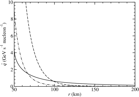
Figure 9: The angle-averaged heating rate per nucleon (solid curve) and the cooling rate per nucleon [dashed ($S=10$) and dot-dashed ($S=20$) curves] in a uniform magnetic field of $B=10^{16}$ G as functions of radius $r$. Compared with Fig. 3, the gain radius decreases significantly from 137 km for $B=0$ to 99 km for $B=10^{16}$ G in the case of $S=10$ but essentially remains at 68 km in the case of $S=20$.

While the angular dependence of the heating rate has some interesting dynamic effects as discussed above, it only introduces minor perturbation on the position of the gain radius. To very good approximation, one may use the angular average of the heating rate [obtained effectively by dropping the terms involving $\cos\theta$ in Eq. (41)] in determining the gain radius. The angle-averaged heating rate for $Y_{e}=0.5$ is shown as a function of $r$ (solid curve) in Fig. 9. In the same figure, we also show the cooling rate $\dot{q}_{c}(B=10^{16}\ \mathrm{G})$ as a function of $r$ using $T(r)$ in Eq. (16) and $Y_{e}=0.5$ for $S=10$ (dashed curve) and $S=20$ (dot-dashed curve), respectively. By comparing Figs. 3 and 9, it can be seen that the gain radius decreases significantly from 137 km for $B=0$ to 99 km for $B=10^{16}$ G in the case of $S=10$ but essentially remains at 68 km in the case of $S=20$. This is because the magnetic field greatly reduces $\eta_{e}$ (see Fig. 4b), and hence, the cooling rate (see Fig. 8a) for $S=10$. But for $S=20$, $\eta_{e}$ is already small for $B=0$ (see Fig. 4b) and reduction of $\eta_{e}$ by the magnetic field does not change the cooling rate significantly (see Fig. 8a). Numerical models Rampp and Janka (2000); Liebend rfer et al. (2001) show that the material below the stalled shock initially has $S\sim 10$. Taking $T(r)$ in Eq. (16), $Y_{e}=0.5$, and $S=10$, we calculate the gain radius as a function of $B$ and show the results in Fig. 10. It can be seen that magnetic fields of $B\sim 10^{16}$ G or larger significantly decrease the gain radius, thereby enhancing the net heating below the stalled shock. Consequently, the shock may be revived more efficiently (i.e., within a shorter time) to make an explosion.

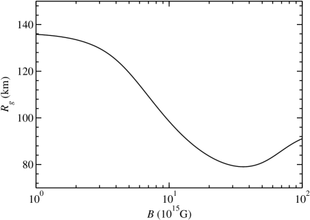
Figure 10: The gain radius $R_{g}$ as a function of magnetic field strength $B$ for a uniform magnetic field ($Y_{e}=0.5$ and $S=10$). The gain radius for $B\sim 10^{15}$ G approaches that for $B=0$.

IV.2 Dipole Field

As a second example, we consider the magnetic field of a dipole in the $z$-direction:

$$\mathbf{B}=B_{0}\left(\frac{R_{\nu}}{r}\right)^{3}(2\cos\theta\,\mathbf{\hat{r}}+\sin\theta\,\mathbf{\hat{\bm{\theta}}}).$$ (43)

The heating and cooling rates in a uniform field discussed in Sec. III can be adapted to the case of a dipole field in a straightforward manner. The strength of the magnetic field to be used in the expressions for $\chi$ [Eq. (22)] and $E_{e}(n,p_{ez})$ [Eq. (25)] is now

$$B(r,\theta)=B_{0}\left(\frac{R_{\nu}}{r}\right)^{3}\sqrt{1+3\cos^{2}\theta}.$$ (44)

In addition, the integration over the neutrino solid angle (see Fig. 7) to obtain the heating rate is changed to

$$\int\cos\Theta_{\nu}\mathrm{d}\Omega_{\nu}=2\pi(R_{\nu}/r)^{2}\frac{\cos\theta}{\sqrt{1+3\cos^{2}\theta}}.$$ (45)

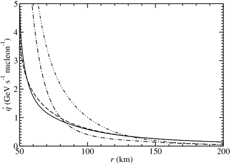
Figure 11: The heating rate per nucleon [dashed ($\cos\theta=0$) and solid ($\cos\theta=1$) curves] and the cooling rate per nucleon [dot-dot-dashed ($\cos\theta=0$) and dot-dashed ($\cos\theta=1$) curves] in a dipole magnetic field as functions of radius $r$ ($Y_{e}=0.5$ and $S=10$). The dipole field has strength $B(r,\theta)=B_{0}(R_{\nu}/r)^{3}\sqrt{1+3\cos^{2}\theta}$ with $B_{0}=5\times 10^{16}$ G.

For illustration, we take $B_{0}=5\times 10^{16}$ G and show the heating rate as a function of $r$ for $\cos\theta=0$ (dashed curve) and $\cos\theta=1$ (solid curve), respectively, in Fig. 11. In the same figure, we also show the corresponding cooling rate using $T(r)$ in Eq. (16), $Y_{e}=0.5$, and $S=10$ [dot-dot-dashed ($\cos\theta=0$) and dot-dashed ($\cos\theta=1$) curves]. It can be seen that the gain radius differs significantly for $\cos\theta=0$ and 1. For a close examination, we show the gain radius $R_{g}$ as a function of $\cos\theta$ (solid curve) in Fig. 12. Compared with $R_{g}=137$ km for $B=0$ (dashed curve), $R_{g}$ is substantially reduced to $\sim 80$ km close to the north and south poles of the magnetic field ($|\cos\theta|\sim 1$). This reduction in $R_{g}$ is somewhat larger than that for the uniform magnetic field discussed above. This is because the strength of the dipole field at $r\sim 100$ km in the polar directions is somewhat larger than the strength of $B=10^{16}$ G taken for the uniform field. By comparison, $R_{g}$ only decreases slightly from 137 km for $B=0$ to 131 km near the equator of the dipole field ($|\cos\theta|\ll 1$). This is because at a given $r$, the strength of a dipole field for $|\cos\theta|\ll 1$ is weaker than that for $|\cos\theta|\sim 1$ by a factor of $\sim 2$ [see Eq. (44)].

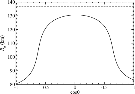
Figure 12: The gain radius $R_{g}$ as a function of $\cos\theta$ (solid curve) for the dipole magnetic field in Fig. 11. Compared with $R_{g}=137$ km for $B=0$ (dashed curve), $R_{g}$ is substantially reduced to $\sim 80$ km close to the north and south poles of the magnetic field ($|\cos\theta|\sim 1$).

The gain radius for $|\cos\theta|\sim 1$ is significantly smaller than that for $|\cos\theta|\ll 1$ in the case of a dipole field. This indicates that the explosion is very likely to occur first in the polar directions of the magnetic field. Note that the ejecta in the north and south poles tend to kick the protoneutron star in opposite directions. However, there would be a net kick as the heating rate differs for $\cos\theta=-1$ and 1. This can be seen from Fig. 12, which shows a small difference in the gain radius for $\cos\theta=-1$ ($R_{g}=80$ km) and $\cos\theta=1$ ($R_{g}=83$ km). Thus, we expect that the possible kick received by the protoneutron star is similar for both the uniform and the dipole fields discussed here.

V Conclusions

We have calculated the rates of heating and cooling due to the neutrino processes in Eqs. (1) and (2) in strong magnetic fields. We find that for $B\sim 10^{16}$ G, the main effect of magnetic fields is to change the equations of state through the phase space of $e^{-}$ and $e^{+}$, which differs from the classical case due to quantization of the motion of $e^{-}$ and $e^{+}$ perpendicular to the magnetic field. As a result, the cooling rate can be greatly reduced by magnetic fields of $\sim 10^{16}$ G for typical conditions ($S\sim 10$) below the stalled shock and a nonuniform protoneutron star magnetic field (e.g., a dipole field) can introduce a large angular dependence of the cooling rate. In addition, strong magnetic fields always lead to an angle-dependent heating rate by polarizing the spin of $n$ and $p$. The decrease in the cooling rate for magnetic fields of $\sim 10^{16}$ G decreases the gain radius and increases the net heating below the stalled shock. We conclude that if magnetic fields of $B\sim 10^{16}$ G exist within $\sim 100$ km of the protoneutron star, the shock can be revived more efficiently (i.e., within a shorter time) to make an explosion. In addition, the anisotropy in the heating rate induced by strong magnetic fields and that in the cooling rate induced by strong nonuniform (e.g., dipole-like) magnetic fields may lead to significant asymmetry in the bulk motion of the material below the stalled shock, eventually producing an asymmetric supernova explosion. We speculate that this may be one of the mechanisms for producing the observed pulsar kick velocities. Obviously, a full treatment of magnetic fields during the formation of a protoneutron star and during the supernova process in general greatly increases the complexity of an already difficult problem. Nevertheless, we hope that the interesting effects of strong magnetic fields discussed here would help to motivate the eventual inclusion of magnetic fields in supernova models.

Appendix A Equations of State

The relevant equations of state concern the net electron number density $(n_{e^{-}}-n_{e^{+}})$ [Eq. (17)] and the total entropy per nucleon $S$ [Eq. (18)]. The photon contribution $S_{\gamma}$ to $S$ is:

$$S_{\gamma}=\frac{4\pi^{2}}{45}\left(\frac{m_{N}}{\rho}\right)T^{3}=1.9\left(\frac{T}{\textrm{MeV}}\right)^{3}\left(\frac{10^{8}\,\textrm{g}\,\textrm{cm}^{-3}}{\rho}\right).$$ (46)

For the conditions in the region of interest, nucleons are nondegenerate and nonrelativistic. So their contribution $S_{N}$ to $S$ is:

$$S_{N} = \frac{5}{2}+Y_{n}\ln\left[\frac{2m_{N}}{\rho Y_{n}}\left(\frac{m_{N}T}{2\pi}\right)^{3/2}\right]+Y_{p}\ln\left[\frac{2m_{N}}{\rho Y_{p}}\left(\frac{m_{N}T}{2\pi}\right)^{3/2}\right]$$ (47)

$$= 11.5+\ln\left[\left(\frac{T}{\textrm{MeV}}\right)^{3/2}\left(\frac{10^{8}\,\textrm{g}\,\textrm{cm}^{-3}}{\rho}\right)\right]-Y_{e}\ln Y_{e}-(1-Y_{e})\ln(1-Y_{e}),$$

where we have used $Y_{n}=1-Y_{e}$ and $Y_{p}=Y_{e}$. The above expressions for $S_{\gamma}$ and $S_{N}$ are valid for both the case of no magnetic field and the case of magnetic fields of $B\sim 10^{16}$ G considered here.

In the absence of magnetic field, the general expressions for the number densities $n_{e^{\pm}}$, energy densities $\varepsilon_{e^{\pm}}$, and pressure $P_{e^{\pm}}$ of $e^{+}$ and $e^{-}$ are:

$$n_{e^{\pm}} = \frac{1}{\pi^{2}}\int_{0}^{\infty}\frac{p_{e^{\pm}}^{2}}{\exp[(E_{e^{\pm}}/T)\pm\eta_{e}]+1}\,\mathrm{d}p_{e^{\pm}}$$ (48)

$$= \frac{T^{3}}{\pi^{2}}\int_{0}^{\infty}\frac{x^{2}}{\exp\left[\sqrt{x^{2}+(m_{e}/T)^{2}}\pm\eta_{e}\right]+1}\,\mathrm{d}x,$$

$$\varepsilon_{e^{\pm}} = \frac{1}{\pi^{2}}\int_{0}^{\infty}\frac{E_{e^{\pm}}p_{e^{\pm}}^{2}}{\exp[(E_{e^{\pm}}/T)\pm\eta_{e}]+1}\,\mathrm{d}p_{e^{\pm}}$$ (49)

$$= \frac{T^{4}}{\pi^{2}}\int_{0}^{\infty}\frac{x^{2}\sqrt{x^{2}+(m_{e}/T)^{2}}}{\exp\left[\sqrt{x^{2}+(m_{e}/T)^{2}}\pm\eta_{e}\right]+1}\,\mathrm{d}x,$$

and

$$P_{e^{\pm}} = \frac{1}{3\pi^{2}}\int_{0}^{\infty}\frac{p_{e^{\pm}}^{4}/E_{e^{\pm}}}{\exp[(E_{e^{\pm}}/T)\pm\eta_{e}]+1}\,\mathrm{d}p_{e^{\pm}}$$ (50)

$$= \frac{T^{4}}{3\pi^{2}}\int_{0}^{\infty}\frac{x^{4}/\sqrt{x^{2}+(m_{e}/T)^{2}}}{\exp\left[\sqrt{x^{2}+(m_{e}/T)^{2}}\pm\eta_{e}\right]+1}\,\mathrm{d}x.$$

In Eqs. (48)–(50), the upper sign is for $e^{+}$ and the lower sign for $e^{-}$.

In magnetic fields, the energy levels and the phase space of $e^{+}$ and $e^{-}$ are changed [see Eqs. (25) and (27)]. The corresponding expressions for $n_{e^{\pm}}$, $\varepsilon_{e^{\pm}}$, and $P_{e^{\pm}}$ are:

$$n_{e^{\pm}} = \frac{eB}{2\pi^{2}}\sum_{n=0}^{\infty}g_{n}\int_{0}^{\infty}\frac{1}{\exp[(E_{e^{\pm}}/T)\pm\eta_{e}]+1}\,\mathrm{d}p_{e^{\pm}z}$$ (51)

$$= \frac{eBT}{2\pi^{2}}\sum_{n=0}^{\infty}g_{n}\int_{0}^{\infty}\frac{1}{\exp\left\{\sqrt{x^{2}+[(m_{e}^{2}+2neB)/T^{2}]}\pm\eta_{e}\right\}+1}\,\mathrm{d}x,$$

$$\varepsilon_{e^{\pm}} = \frac{eB}{2\pi^{2}}\sum_{n=0}^{\infty}g_{n}\int_{0}^{\infty}\frac{E_{e^{\pm}}}{\exp[(E_{e^{\pm}}/T)\pm\eta_{e}]+1}\,\mathrm{d}p_{e^{\pm}z}$$ (52)

$$= \frac{eBT^{2}}{2\pi^{2}}\sum_{n=0}^{\infty}g_{n}\int_{0}^{\infty}\frac{\sqrt{x^{2}+[(m_{e}^{2}+2neB)/T^{2}]}}{\exp\left\{\sqrt{x^{2}+[(m_{e}^{2}+2neB)/T^{2}]}\pm\eta_{e}\right\}+1}\,\mathrm{d}x,$$

and

$$P_{e^{\pm}} = \frac{eB}{2\pi^{2}}\sum_{n=0}^{\infty}g_{n}\int_{0}^{\infty}\frac{p_{e^{\pm}z}^{2}/E_{e^{\pm}}}{\exp[(E_{e^{\pm}}/T)\pm\eta_{e}]+1}\,\mathrm{d}p_{e^{\pm}z}$$ (53)

$$= \frac{eBT^{2}}{2\pi^{2}}\sum_{n=0}^{\infty}g_{n}\int_{0}^{\infty}\frac{x^{2}/\sqrt{x^{2}+[(m_{e}^{2}+2neB)/T^{2}]}}{\exp\left\{\sqrt{x^{2}+[(m_{e}^{2}+2neB)/T^{2}]}\pm\eta_{e}\right\}+1}\,\mathrm{d}x.$$

In Eqs. (51)–(53), the upper sign is for $e^{+}$ and the lower sign for $e^{-}$.

The contributions $S_{e^{\pm}}$ from $e^{+}$ and $e^{-}$ to $S$ can be obtained in terms of $n_{e^{\pm}}$, $\varepsilon_{e^{\pm}}$, and $P_{e^{\pm}}$ as

$$S_{e^{\pm}}=\left(\frac{m_{N}}{\rho}\right)\left[\frac{\varepsilon_{e^{\pm}}+P_{e^{\pm}}}{T}\pm\eta_{e}n_{e^{\pm}}\right].$$ (54)

More specifically,

$$S_{e^{-}}+S_{e^{+}}=\frac{\varepsilon_{e^{-}}+\varepsilon_{e^{+}}+P_{e^{-}}+P_{e^{+}}}{T(\rho/m_{N})}-\eta_{e}Y_{e},$$ (55)

where we have used $n_{e^{-}}-n_{e^{+}}=Y_{e}\rho/m_{N}$.

Appendix B Neutrino processes in strong magnetic fields

A number of studies on neutrino processes in strong magnetic fields exist in the literature. The forward and reverse processes in Eq. (1) have been studied in Refs. Chandra et al. (2002) and Leinson and Pérez (1998) assuming that $e^{-}$ and $p$ are in the ground $(n=0)$ Landau levels. All the four processes in Eqs. (1) and (2) have been studied in Ref. Gvozdev and Ognev (1999) assuming that $e^{-}$ and $e^{+}$ only occupy the ground Landau levels. The forward processes in Eqs. (1) and (2) have been studied in Refs. Roulet (1998) and Lai and Qian (1998) assuming that the magnetic field only affects the phase space of $e^{-}$ and $e^{+}$. Parity violation in the forward process in Eq. (1) has been studied in Ref. Arras and Lai (1999). The cross section of the forward process in Eq. (1) has been calculated in Ref. Bhattacharya and Pal (2003) using an approach similar to ours. In this appendix, we treat the forward and reverse processes in Eqs. (1) and (2) in magnetic fields of $B\sim 10^{16}\,\textrm{G}$. Such fields are strong enough to change the motion of $e^{-}$ and $e^{+}$ but do not affect the description of weak interation (see Sec. III).

Ignoring higher order corrections, we take the effective four-fermion Lagrangian of weak interaction to be

$$\mathcal{L}_{\mathrm{int}}=\frac{G_{F}}{\sqrt{2}}\cos\theta_{C}N_{\alpha}^{\dagger}L^{\alpha}+\mathrm{h.c.},$$ (56)

where $\mathrm{h.c.}$ means the Hermitian conjugation of the first term. In Eq. (56), the leptonic charged current $L^{\alpha}$ has the classical $V-A$ form

$$L^{\alpha}=\bar{\psi}^{e}\gamma^{\alpha}(1-\gamma_{5})\psi^{\nu},$$ (57)

and the nucleonic current $N^{\alpha}$ is

$$N^{\alpha}=\bar{\psi}^{p}\gamma^{\alpha}(f-g\gamma_{5})\psi^{n}.$$ (58)

The form factors $f$ and $g$ in Eq. (58) are taken as constant. In the calculation below, we shall use the Dirac-Pauli representation and take the magnetic field $\mathbf{B}$ to be in the positive z-direction. All the terms of order $m_{N}^{-1}$ and higher are ignored in the calculation.

The wavefunction of a left-handed neutrino with momentum $\mathbf{p}_{\nu}=E_{\nu}(\sin\Theta_{\nu},0,\cos\Theta_{\nu})$ is

$$\psi_{\mathbf{p}_{\nu}}^{\nu}=\frac{e^{i(\mathbf{p}_{\nu}\cdot\mathbf{x}-E_{\nu}t)}}{\sqrt{2}L^{3/2}}\left(\begin{array}[]{c}\sin\frac{\Theta_{\nu}}{2}\\ -\cos\frac{\Theta_{\nu}}{2}\\ -\sin\frac{\Theta_{\nu}}{2}\\ \cos\frac{\Theta_{\nu}}{2}\end{array}\right)=\frac{e^{i(\mathbf{p}_{\nu}\cdot\mathbf{x}-E_{\nu}t)}}{L^{3/2}}U_{\mathbf{p}_{\nu}}^{\nu},$$ (59)

where $L$ is the linear size of the normalization volume. The above wavefunction also applies to a right-handed antineutrino with the same momentum. The wavefunction of a non-relativistic nucleon is

$$\psi_{\mathbf{k}_{n(p)},s_{n(p)}}^{n(p)}=\frac{e^{i(\mathbf{k}_{n(p)}\cdot\mathbf{x}-m_{n(p)}t)}}{L^{3/2}}\left(\begin{array}[]{c}\delta_{s_{n(p)},1}\\ \delta_{s_{n(p)},-1}\\ 0\\ 0\end{array}\right)=\frac{e^{i(\mathbf{k}_{n(p)}\cdot\mathbf{x}-m_{n(p)}t)}}{L^{3/2}}U_{\mathbf{k}_{n(p)},s_{n(p)}}^{n(p)},$$ (60)

where $s_{n(p)}=\pm 1$ denotes the spin state and $\mathbf{k}_{n(p)}$ is the nucleon momentum.

In cylindrical coordinates $(\xi,\phi,z)$, the wavefunction of an electron is

$$\psi_{n,n_{r},p_{ez},s_{e}}^{e^{-}}=\frac{e^{i(p_{ez}z-E_{e}t)}e^{i(n-n_{r})\phi}}{\sqrt{2\pi\lambda^{2}L}}U_{n,n_{r},p_{ez},s_{e}}^{e^{-}},$$ (61)

where $n$ is the quantum number of the Landau level, $n_{r}$ is the quantum number of the gyromotion center, $\lambda=1/\sqrt{eB}$ is a characteristic length scale defined by the strength of the magnetic field, and $s_{e}=\pm 1$ corresponds to the two spin states when the electron is at rest. The spinor $\psi_{n,n_{r},p_{ez},s_{e}}^{e^{-}}$ in Eq. (61) is

$$U_{n,n_{r},p_{ez},s_{e}=1}^{e^{-}}=\frac{1}{\sqrt{2E_{e}(E_{e}+m_{e})}}\left(\begin{array}[]{c}(m_{e}+E_{e})e^{-i\phi}I_{n-1,n_{r}}(\xi^{2}/2\lambda^{2})\\ 0\\ p_{ez}e^{-i\phi}I_{n-1,n_{r}}(\xi^{2}/2\lambda^{2})\\ i\frac{\sqrt{2n}}{\lambda}I_{n,n_{r}}(\xi^{2}/2\lambda^{2})\end{array}\right)$$ (62)

and

$$U_{n,n_{r},p_{ez},s_{e}=-1}^{e^{-}}=\frac{1}{\sqrt{2E_{e}(E_{e}+m_{e})}}\left(\begin{array}[]{c}0\\ (m_{e}+E_{e})I_{n,n_{r}}(\xi^{2}/2\lambda^{2})\\ -i\frac{\sqrt{2n}}{\lambda}e^{-i\phi}I_{n-1,n_{r}}(\xi^{2}/2\lambda^{2})\\ -p_{ez}I_{n,n_{r}}(\xi^{2}/2\lambda^{2})\end{array}\right).$$ (63)

The special function $I_{n,n_{r}}(\eta)$ in the above equations is defined in Ref. Sokolov and Temov (1968), and can be written in terms of the generalized Laguerre polynomial $L_{n_{r}}^{n-n_{r}}(\eta)$ as

$$I_{n,n_{r}}(\eta)=\sqrt{\frac{n_{r}!}{n!}}e^{-\eta/2}\eta^{(n-n_{r})/2}L_{n_{r}}^{n-n_{r}}(\eta).$$ (64)

The electron wavefunction discussed above is the same as given in Ref. Johnson and Lippmann (1949) up to a phase factor [Note that there are a few typos in that reference: Eq. (45) should read $\psi_{n,l}=(-i)^{n}(2^{n+l+1}\pi l!n!)^{-\frac{1}{2}}\lambda^{n-1}\times\cdots$ and Eq. (46) should read $\psi_{n,l}=i^{n}(2^{n-l+1}\pi l!n!)^{-\frac{1}{2}}\lambda^{-1}(\rho/\lambda)^{n-l}\times\cdots$]. The wavefunction of a positron is

$$\psi_{n,n_{r},p_{ez},s_{e}}^{e^{+}}=\frac{e^{-i(p_{ez}z-E_{e}t)}e^{i(n-n_{r})\phi}}{\sqrt{2\pi\lambda^{2}L}}U_{n,n_{r},p_{ez},s_{e}}^{e^{+}},$$ (65)

where

$$U_{n,n_{r},p_{ez},s_{e}=1}^{e^{+}}=\frac{1}{\sqrt{2E_{e}(E_{e}+m_{e})}}\left(\begin{array}[]{c}i\frac{\sqrt{2n}}{\lambda}e^{-i\phi}I_{n-1,n_{r}}(\xi^{2}/2\lambda^{2})\\ -p_{ez}I_{n,n_{r}}(\xi^{2}/2\lambda^{2})\\ 0\\ (m_{e}+E_{e})I_{n,n_{r}}(\xi^{2}/2\lambda^{2})\end{array}\right),$$ (66)

and

$$U_{n,n_{r},p_{ez},s_{e}=-1}^{e^{+}}=\frac{1}{\sqrt{2E_{e}(E_{e}+m_{e})}}\left(\begin{array}[]{c}-p_{ez}e^{-i\phi}I_{n-1,n_{r}}(\xi^{2}/2\lambda^{2})\\ i\frac{\sqrt{2n}}{\lambda}I_{n,n_{r}}(\xi^{2}/2\lambda^{2})\\ -(m_{e}+E_{e})e^{-i\phi}I_{n-1,n_{r}}(\xi^{2}/2\lambda^{2})\\ 0\end{array}\right).$$ (67)

All the wavefunctions are normalized to have one particle in a volume of $L^{3}$.

The scattering matrix of $\nu_{e}+n\rightarrow e^{-}+p$ is

$$i\mathcal{T}_{fi} = \frac{G_{F}\cos\theta_{C}}{\sqrt{2}}\int\bar{\psi}_{\mathbf{k}_{p},s_{p}}^{p}\gamma_{\alpha}(f-g\gamma_{5})\psi_{\mathbf{k}_{n},s_{n}}^{n}\bar{\psi}_{n,n_{r},p_{ez},s_{e}}^{e^{-}}\gamma^{\alpha}(1-\gamma_{5})\psi_{\mathbf{p}_{\nu}}^{\nu}\,\mathrm{d}^{4}x$$ (68)

$$= \frac{G_{F}\cos\theta_{C}}{\sqrt{2}}\frac{1}{\sqrt{2\pi\lambda^{2}}L^{5}}2\pi\delta(E_{e}-E_{\nu}-\Delta)2\pi\delta(k_{pz}+p_{ez}-k_{nz}-p_{\nu z})\mathfrak{M}.$$

In Eq. (68),

$$\mathfrak{M}=\int_{0}^{\infty}\xi\,\mathrm{d}\xi\int_{0}^{2\pi}e^{i\mathbf{w}_{\perp}\cdot\mathbf{x}_{\perp}}e^{-i(n-n_{r})\phi}\bar{U}_{\mathbf{k}_{p},s_{p}}^{p}\gamma_{\alpha}(f-g\gamma_{5})U_{\mathbf{k}_{n},s_{n}}^{n}\bar{U}_{n,n_{r},p_{ez},s_{e}}^{e^{-}}\gamma^{\alpha}(1-\gamma_{5})U_{\mathbf{p}_{\nu}}^{\nu}\,\mathrm{d}\phi,$$ (69)

where the subscript “$\perp$” denotes a vector in the xy-plane and $\mathbf{w}_{\perp}=(\mathbf{k}_{n}+\mathbf{p}_{\nu}-\mathbf{k}_{p})_{\perp}$. Similarly, the scattering matrix of $e^{+}+n\rightarrow\bar{\nu}_{e}+p$ is,

$$i\mathcal{T}_{fi}^{\prime} = \frac{G_{F}\cos\theta_{C}}{\sqrt{2}}\int\bar{\psi}_{\mathbf{k}_{p},s_{p}}^{p}\gamma_{\alpha}(f-g\gamma_{5})\psi_{\mathbf{k}_{n},s_{n}}^{n}\bar{\psi}_{n,n_{r},p_{ez},s_{e}}^{e^{+}}\gamma^{\alpha}(1-\gamma_{5})\psi_{\mathbf{p}_{\nu}}^{\bar{\nu}}\,\mathrm{d}^{4}x$$ (70)

$$= \frac{G_{F}\cos\theta_{C}}{\sqrt{2}}\frac{1}{\sqrt{2\pi\lambda^{2}}L^{5}}2\pi\delta(E_{\nu}-E_{e}-\Delta)2\pi\delta(k_{pz}+p_{\nu z}-k_{nz}-p_{ez})\mathfrak{M}^{\prime}.$$

In Eq. (70),

$$\mathfrak{M}^{\prime}=\int_{0}^{\infty}\xi\,\mathrm{d}\xi\int_{0}^{2\pi}e^{i\mathbf{w}^{\prime}_{\perp}\cdot\mathbf{x}_{\perp}}e^{-i(n-n_{r})\phi}\bar{U}_{\mathbf{k}_{p},s_{p}}^{p}\gamma_{\alpha}(f-g\gamma_{5})U_{\mathbf{k}_{n},s_{n}}^{n}\bar{U}_{n,n_{r},p_{ez},s_{e}}^{e^{+}}\gamma^{\alpha}(1-\gamma_{5})U_{\mathbf{p}_{\nu}}^{\bar{\nu}}\,\mathrm{d}\phi,$$ (71)

where $\mathbf{w}^{\prime}_{\perp}=(\mathbf{k}_{n}-\mathbf{k}_{p}-\mathbf{p}_{\nu})_{\perp}$. The scattering matrices of $e^{-}+p\rightarrow n+\nu_{e}$ and $\bar{\nu}_{e}+p\rightarrow n+e^{+}$ are the Hermitian conjugate of those in Eqs. (68) and (70), respectively.

Based on formula 8.411.1 in Ref. Gradshteyn and Ryzhik (1980), we obtain

$$\int_{0}^{2\pi}e^{i\mathbf{w}_{\perp}\cdot\mathbf{x}_{\perp}-i(n-n_{r})\phi}\,\mathrm{d}\phi = \int_{0}^{2\pi}e^{iw_{\perp}\rho\cos(\phi-\phi_{0})-i(n-n_{r})\phi}\,\mathrm{d}\phi$$ (72)

$$= 2\pi i^{n-n_{r}}e^{-i(n-n_{r})\phi_{0}}J_{n-n_{r}}(w_{\perp}\xi),$$

where $\phi_{0}$ is the azimuthal angle of $\mathbf{w}_{\perp}$, and $J_{n}(\eta)$ is the Bessel function of order $n$. Using this and formula 7.421.4 in Ref. Gradshteyn and Ryzhik (1980)

$$\int_{0}^{\infty}x^{\nu+1}e^{-\beta x^{2}}L_{n}^{\nu}(\alpha x^{2})J_{\nu}(xy)\,\mathrm{d}x=2^{-\nu-1}\beta^{-\nu-n-1}(\beta-\alpha)^{n}y^{\nu}e^{-y^{2}/4\beta}L_{n}^{\nu}\left(\frac{\alpha y^{2}}{4\beta(\alpha-\beta)}\right),$$ (73)

one can prove that

$$\int_{0}^{\infty}\xi\,\mathrm{d}\xi\int_{0}^{2\pi}e^{i\mathbf{w}_{\perp}\cdot\mathbf{x}_{\perp}}e^{-i(n-n_{r})\phi}I_{n,n_{r}}(\xi^{2}/2\lambda^{2})\,\mathrm{d}\phi$$

$$= i^{n+n_{r}}e^{-i(n-n_{r})\phi_{0}}4\pi\lambda^{2}I_{n,n_{r}}(2\lambda^{2}w_{\perp}^{2}).$$ (74)

Using Eq. (74), we obtain $\left|\mathfrak{M}\right|^{2}$ of the forward and reverse processes in Eq. (1) as

$$\left|\mathfrak{M}\right|_{s_{p}=1,s_{n}=1}^{2} = 4(2\pi\lambda^{2})^{2}\Big{[}(f+g)^{2}\left(1+v_{ez}\right)(1+\cos\Theta_{\nu})I_{n,n_{r}}^{2}(2\lambda^{2}w_{\perp}^{2})$$ (75a)

$$+(f-g)^{2}\left(1-v_{ez}\right)(1-\cos\Theta_{\nu})I_{n-1,n_{r}}^{2}(2\lambda^{2}w_{\perp}^{2})$$

$$+2(f^{2}-g^{2})\frac{\sqrt{2neB}}{E_{e}}\cos\phi_{0}\sin\Theta_{\nu}I_{n,n_{r}}(2\lambda^{2}w_{\perp}^{2})I_{n-1,n_{r}}(2\lambda^{2}w_{\perp}^{2})\Big{]},$$

$$\left|\mathfrak{M}\right|_{s_{p}=1,s_{n}=-1}^{2} = 16(2\pi\lambda^{2})^{2}g^{2}\left(1+v_{ez}\right)(1-\cos\Theta_{\nu})I_{n,n_{r}}^{2}(2\lambda^{2}w_{\perp}^{2}),$$ (75b)

$$\left|\mathfrak{M}\right|_{s_{p}=-1,s_{n}=1}^{2} = 16(2\pi\lambda^{2})^{2}g^{2}\left(1-v_{ez}\right)(1+\cos\Theta_{\nu})I_{n-1,n_{r}}^{2}(2\lambda^{2}w_{\perp}^{2}),$$ (75c)

$$\left|\mathfrak{M}\right|_{s_{p}=-1,s_{n}=-1}^{2} = 4(2\pi\lambda^{2})^{2}\Big{[}(f-g)^{2}\left(1+v_{ez}\right)(1+\cos\Theta_{\nu})I_{n,n_{r}}^{2}(2\lambda^{2}w_{\perp}^{2})$$ (75d)

$$+(f+g)^{2}\left(1-v_{ez}\right)(1-\cos\Theta_{\nu})I_{n-1,n_{r}}^{2}(2\lambda^{2}w_{\perp}^{2})$$

$$+2(f^{2}-g^{2})\frac{\sqrt{2neB}}{E_{e}}\cos\phi_{0}\sin\Theta_{\nu}I_{n,n_{r}}(2\lambda^{2}w_{\perp}^{2})I_{n-1,n_{r}}(2\lambda^{2}w_{\perp}^{2})\Big{]},$$

where $v_{ez}=p_{ez}/E_{e}$ is the longitudinal velocity of the electron. The corresponding expressions of $\left|\mathfrak{M}^{\prime}\right|^{2}$, which apply to the forward and reverse processes in Eq. (2), can be obtained from the above expressions of $\left|\mathfrak{M}\right|^{2}$ by changing the signs of the terms proportional to $(f^{2}-g^{2})$ and replacing $\mathbf{w}_{\perp}$ with $\mathbf{w}^{\prime}_{\perp}$.

The cross section of $\nu_{e}+n\rightarrow e^{-}+p$ is

$$\sigma_{\nu_{e}n}(B) = \sum_{s_{p}}\int\frac{L^{3}\mathrm{d}^{3}k_{p}}{(2\pi)^{3}}\sum_{n,n_{r},s_{e}}\int\frac{L\mathrm{d}p_{ez}}{2\pi}\frac{1}{L^{-3}L^{-3}}\frac{G_{F}^{2}\cos^{2}\theta_{C}}{2}$$ (76)

$$\times 2\pi\delta(E_{e}-E_{\nu}-\Delta)2\pi\delta(k_{pz}+p_{ez}-k_{nz}-p_{\nu z})\frac{TL}{2\pi\lambda^{2}L^{10}}\frac{\left|\mathfrak{M}\right|^{2}}{TL^{3}}.$$

In this appendix only, the symbol $T$ deontes the duration of a process such as $\nu_{e}+n\rightarrow e^{-}+p$. Evaluation of $\sigma_{\nu_{e}n}(B)$ can be simplified using the summation rule Sokolov and Temov (1968) for the special function $I_{n,n_{r}}(2\lambda^{2}w_{\perp}^{2})$ in $\left|\mathfrak{M}\right|^{2}$,

$$\sum_{n_{r}}I_{n,n_{r}}(\eta)I_{n^{\prime}n_{r}}(\eta)=\delta_{n,n^{\prime}},$$ (77)

where $\delta_{n,n^{\prime}}$ is the Kronecker delta function. A difficulty in evaluation of $\sigma_{\nu_{e}n}(B)$ is that the integrand in Eq. (76) is independent of $(\mathbf{k}_{p})_{\perp}$ in the infinite nucleon mass limit and the integral diverges. Another difficulty is that there is a remaining factor of $L^{-2}$. These difficulties arise because $e^{-}$ does not have definite transverse canonical momenta and we drop all the terms of order $m_{N}^{-1}$ and higher. However, $e^{-}$ has definite transverse kinetic momentum squared

$$(\bm{\pi}_{e})_{\perp}^{2}=\left(p_{ex}-\frac{y}{2\lambda^{2}}\right)^{2}+\left(p_{ey}+\frac{x}{2\lambda^{2}}\right)^{2}=(2n+1)eB.$$ (78)

The limit on $x$ and $y$ then corresponds to a limit of $L/2\lambda^{2}$ on $p_{ex}$ and $p_{ey}$. Thus, we take

$$\int\frac{L^{2}\mathrm{d}k_{px}\,\mathrm{d}k_{py}}{(2\pi)^{2}}\longrightarrow\frac{L^{4}}{4\left(2\pi\lambda^{2}\right)^{2}}.$$ (79)

Using Eqs. (75), (76), (77), and (79), we obtain

$$\sigma_{\nu_{e}n}(B) = \sigma_{B}^{(1)}\left[1+2\chi_{n}\frac{(f+g)g}{f^{2}+3g^{2}}\cos\Theta_{\nu}\right]$$ (80)

$$+\sigma_{B}^{(2)}\left[\frac{f^{2}-g^{2}}{f^{2}+3g^{2}}\cos\Theta_{\nu}+2\chi_{n}\frac{(f-g)}{f^{2}+3g^{2}}\right],$$

where

$$\sigma_{B}^{(1)} = \frac{G_{F}^{2}\cos^{2}\theta_{C}}{2\pi}(f^{2}+3g^{2})eB\sum_{n=0}^{n_{\textrm{max}}}\frac{g_{n}E_{e}}{\sqrt{E_{e}^{2}-m_{e}^{2}-2neB}},$$ (81)

$$\sigma_{B}^{(2)} = \frac{G_{F}^{2}\cos^{2}\theta_{C}}{2\pi}(f^{2}+3g^{2})eB\frac{E_{e}}{\sqrt{E_{e}^{2}-m_{e}^{2}}},$$ (82)

and $\chi_{n}$ is the net polarization of the neutron in the initial state. In Eq. (81), $g_{n}$ denotes the degeneracy of Landau level $n$ for $e^{-}$. The cross section of $\bar{\nu}_{e}+p\rightarrow e^{+}+n$ can be obtained in a similar way as

$$\sigma_{\bar{\nu}_{e}p}(B) = \sigma_{B}^{(1)}\left[1+2\chi_{p}\frac{(f-g)g}{f^{2}+3g^{2}}\cos\Theta_{\nu}\right]$$ (83)

$$+\sigma_{B}^{(2)}\left[\frac{f^{2}-g^{2}}{f^{2}+3g^{2}}\cos\Theta_{\nu}+2\chi_{p}\frac{(f+g)}{f^{2}+3g^{2}}\right].$$

As $e^{-}$ does not have definite velocity, we calculate the volume reaction rate instead of the cross section for $e^{-}+p\rightarrow\nu_{e}+n$. To illustrate the dependence on the direction of the outgoing $\nu_{e}$, we first calculate the differential volume reaction rate

$$\frac{\mathrm{d}\Gamma_{e^{-}p}(B)}{\mathrm{d}\!\cos\Theta_{\nu}} = \overline{\sum_{i}}\sum_{s_{n}}\int\frac{L^{3}\mathrm{d}^{3}k_{n}}{(2\pi)^{3}}\int\frac{L^{3}2\pi E_{\nu}^{2}\mathrm{d}E_{\nu}}{(2\pi)^{3}}\frac{1}{L^{-3}L^{-3}}\frac{G_{F}^{2}\cos^{2}\theta_{C}}{2}$$ (84)

$$\times 2\pi\delta(E_{\nu}+\Delta-E_{e})2\pi\delta(p_{\nu z}+k_{nz}-p_{ez}-k_{pz})\frac{TL}{2\pi\lambda^{2}L^{10}}\frac{\left|\mathfrak{M}\right|^{2}}{TL^{3}}.$$

In Eq. (84),

$$\overline{\sum_{i}}=\frac{1}{g_{n}}\sum_{s_{e}}\,\frac{1}{2}\sum_{p_{ez}}\,\frac{2\pi\lambda^{2}}{L^{2}}\sum_{n_{r}},$$ (85)

which represents the average over all possible initial $e^{-}$ states with a given energy $E_{e}$ and a given Landau level quantum number $n$. Using Eqs. (75), (79) (with $k_{px(y)}$ replaced with $k_{nx(y)}$), (84), and (85), we obtain

$$\frac{\mathrm{d}\Gamma_{e^{-}p}(B)}{\mathrm{d}\!\cos\Theta_{\nu}} = \frac{\Gamma_{eN}^{(0)}}{2}\left[1+2\chi_{p}\frac{(f-g)g}{f^{2}+3g^{2}}\cos\Theta_{\nu}\right]$$ (86)

$$+\delta_{n,0}\frac{\Gamma_{eN}^{(0)}}{2}\left[\frac{f^{2}-g^{2}}{f^{2}+3g^{2}}\cos\Theta_{\nu}+2\chi_{p}\frac{(f+g)g}{f^{2}+3g^{2}}\right],$$

where

$$\Gamma_{eN}^{(0)}=\frac{G_{F}^{2}\cos^{2}\theta_{C}}{2\pi}(f^{2}+3g^{2})E_{\nu}^{2}$$ (87)

is the volume reaction rate without magnetic field. Integrating (86) over $\cos\Theta_{\nu}$, we have

$$\Gamma_{e^{-}p}(B)=\Gamma_{eN}^{(0)}\left[1+\delta_{n,0}\,2\chi_{p}\frac{(f+g)g}{f^{2}+3g^{2}}\right].$$ (88)

The volume reaction rate of $e^{+}+n\rightarrow\bar{\nu}_{e}+p$ can be obtained in a similar way as

$$\frac{\mathrm{d}\Gamma_{e^{+}n}(B)}{\mathrm{d}\!\cos\Theta_{\nu}} = \frac{\Gamma_{eN}^{(0)}}{2}\left[1+2\chi_{n}\frac{(f+g)g}{f^{2}+3g^{2}}\cos\Theta_{\nu}\right]$$ (89)

$$+\delta_{n,0}\frac{\Gamma_{eN}^{(0)}}{2}\left[\frac{f^{2}-g^{2}}{f^{2}+3g^{2}}\cos\Theta_{\nu}+2\chi_{n}\frac{(f-g)g}{f^{2}+3g^{2}}\right],$$

and

$$\Gamma_{e^{+}n}(B)=\Gamma_{eN}^{(0)}\left[1+\delta_{n,0}\,2\chi_{n}\frac{(f-g)g}{f^{2}+3g^{2}}\right].$$ (90)

References

Bethe (1990)
H. A. Bethe,
Rev. Mod. Phys. 62,
801 (1990).
Bethe and Wilson (1985)
H. A. Bethe and
J. R. Wilson,
Astrophys. J. 295,
14 (1985).
Rampp and Janka (2000)
M. Rampp and
H.-T. Janka,
Astrophys. J. 539,
L33 (2000), eprint astro-ph/0005438.
Liebend rfer et al. (2001)
M. Liebend rfer,
A. Mezzacappa,
F.-K. Thielemann,
O. E. Messer,
W. R. Hix, and
S. W. Bruenn,
Phys. Rev. D 63,
103004 (2001), eprint astro-ph/0006418.
Fryer and Warren (2002)
C. L. Fryer and
M. S. Warren,
Astrophys. J. 574,
L65 (2002), eprint astro-ph/0206017.
Kouveliotou et al. (1999)
C. Kouveliotou,
T. Strohmayer,
K. Hurley,
J. van Paradijs,
M. H. Finger,
S. Dieters,
P. Woods,
C. Thompson, and
R. C. Duncan,
Astrophys. J. 510,
L115 (1999), eprint astro-ph/9809140.
Gotthelf et al. (1999)
E. V. Gotthelf,
G. Vasisht, and
T. Dotani,
Astrophys. J. 522,
L49 (1999), eprint astro-ph/9906122.
Ibrahim et al. (2003)
A. I. Ibrahim,
J. H. Swank, and
W. Parke,
Astrophys. J. 584,
L17 (2003), eprint astro-ph/0210515.
Lai (2001)
D. Lai, Rev.
Mod. Phys. 73, 629
(2001), eprint astro-ph/0009333.
Khokhlov et al. (1999)
A. M. Khokhlov,
P. A. Höflich,
E. S. Oran,
J. C. Wheeler,
L. Wang, and
A. Y. Chtchelkanova,
Astrophys. J. 524,
107 (1999), eprint astro-ph/9904419.
Raffelt (1996)
G. G. Raffelt,
Stars as Laboratories for Fundamental Physics
(University of Chicago, Chicago,
1996).