Estimating the bispectrum of the Very Small Array data

Abstract

We estimate the bispectrum of the Very Small Array data from the compact and extended configuration observations released in December 2002, and compare our results to those obtained from Gaussian simulations. There is a slight excess of large bispectrum values for two individual fields, but this does not appear when the fields are combined. Given our expected level of residual point sources, we do not expect these to be the source of the discrepancy. Using the compact configuration data, we put an upper limit of 5400 on the value of $f_{\mathrm{NL}}$, the non-linear coupling parameter, at 95 per cent confidence. We test our bispectrum estimator using non-Gaussian simulations with a known bispectrum, and recover the input values.

1 Introduction

Currently-favoured cosmological theories predict that the primordial fluctuations in the cosmic microwave background (CMB) obey Gaussian statistics to a high degree. The majority of inflationary scenarios imply a level of non-Gaussianity that is unlikely to be detectable by any forthcoming experiment (Acquaviva et al., 2003; Maldacena, 2003), although non-linear gravitational evolution may result in detectable non-Gaussianity from the initially almost-Gaussian fluctuations (Bartolo, Matarrese & Riotto, 2004). Any convincing evidence for a departure from primordial Gaussianity would therefore play a very significant role in constraining theories of inflation. However, the dominant contributions to non-Gaussianity in the CMB are expected to come from secondary effects such as gravitational lensing, reionization, the Sunyaev-Zel’dovich effect, and from the local Universe. These effects are of varying significance, depending on the scale. Coupling between lensing and the Sunyaev-Zel’dovich effect tends to dominate over primordial non-Gaussianity on small scales (Goldberg & Spergel, 1999). The effects of dust and gas clouds are very dependent on the region of sky observed. The Very Small Array (VSA) fields were carefully chosen to minimise contamination from Galactic emission and bright radio sources, and the signal from Galactic foregrounds is thought to be much less than the primordial CMB signal, with the amount of contamination smaller on smaller scales (Taylor et al., 2003). The recent results from the Wilkinson Microwave Anisotropy Probe (WMAP; Komatsu et al. 2003) have considerably tightened the constraints on primordial non-Gaussianity, whilst detecting a non-Gaussian signal arising from residual point sources. The non-Gaussian signal that was found in the bispectrum of the COBE data (Ferreira, Magueijo & Górski, 1998) has not been replicated in the WMAP data and is now believed to be a result of systematic errors (Magueijo & Medeiros, 2003). The VSA has a dedicated point source subtractor, in order to remove all the sources above a certain minimum flux level, so that the residual contribution from unsubtracted sources is less than the flux sensitivity (Taylor et al., 2003).

Whilst we may therefore have little basis for expecting to detect primordial non-Gaussianity in the VSA data, it is important to test the data nevertheless, if only to validate the assumption of Gaussianity which is made during the estimation of the power spectrum and its errors (Hobson & Maisinger, 2002). Currently the published VSA data extend past $\ell=1400$ (Grainge et al., 2003), in comparison with the current WMAP data which do not go beyond $\ell=900$, so we are probing the fluctuations at higher resolution. Testing the data may also help to ascertain whether point source subtraction has been performed satisfactorily, and to see if there is any contamination by foreground sources.

The VSA data have already been tested for non-Gaussianity using a variety of statistics in the map plane, and in the visibility plane by adopting a non-Gaussian likelihood function. The results are presented in Savage et al. (2004). Here, we use the bispectrum, the three-point statistic in the visibility plane.

In Section 2 we discuss the statistics of CMB temperature fluctuations, and how the level of non-Gaussianity can be measured by the bispectrum. We then give a brief overview of the VSA in Section 3, particularly with reference to the point source subtraction technique, and present an approximate expression for the measured visibility three-point function, taking into account the convolution with the primary beam. An exact expression is derived in Appendix C. In Section 4.1 we describe our method for estimating the bispectrum of the VSA data, which we have tested by producing non-Gaussian simulations as described in Section 4.2. We then discuss a method for comparing the results to Gaussian simulations in Section 4.3 and present our results. In Sections 4.4 and 4.5 we consider the effect of point sources on the bispectrum, and look at the feasibility of detecting them in this way. Finally, in Section 4.6 we investigate the constraints that the VSA data are able to place on primordial non-Gaussianity. In the appendices we discuss optimal cubic bispectrum estimators, and the effect of the primary beam on the observed bispectrum from interferometric data.

2 Statistics of CMB temperature fluctuations

2.1 Power spectrum

Assuming full sky coverage, the temperature fluctuations of the CMB can be decomposed into spherical harmonics ($Y_{\ell m}$), and hence expressed as

$$\frac{\Delta T}{T}\left(\mn@boldsymbol{\hat{n}}\right)=\sum_{\ell,m}a_{\ell m}Y_{\ell m}\left(\mn@boldsymbol{\hat{n}}\right).$$ (1)

Here, $T=T_{0}$, the mean temperature of the CMB. Rotational invariance demands that $\left\langle a_{\ell_{1}m_{1}}a^{*}_{\ell_{2}m_{2}}\right\rangle=C_{\ell_{1}}\delta_{\ell_{1}\ell_{2}}\delta_{m_{1}m_{2}},$ where the brackets denote the ensemble average value. The values of the $C_{\ell}$ represent the power spectrum of the CMB, which has been the major focus of attention in CMB studies. The measured values of the $C_{\ell}$ will differ slightly from the ensemble-averaged $C_{\ell}$ due to instrument noise and cosmic variance; if the $a_{\ell m}$ are each drawn independently from a Gaussian distribution, with mean 0 and variance $C_{\ell}$, then the measured $C_{\ell}$ will be drawn from a $\chi^{2}$ distribution, with an intrinsic variance equal to $\frac{2C_{\ell}^{2}}{2\ell+1}$. Therefore, particularly at low $\ell$, there will always be an uncertainty as to the true value of the $C_{\ell}$, independent of the technical difficulties of experimental measurement.

2.2 Higher-order statistics

If the temperature fluctuations of the CMB are Gaussian, the power spectrum completely describes the statistics. However, if there is a departure from Gaussianity, higher-order statistics are needed for a full description. In principle there is an infinite number of ways in which the CMB could be non-Gaussian, and therefore the optimal statistic to use depends on the type of non-Gaussianity present. If we are looking for a particular signal we can use a statistic which is tailored for optimal detection of that signal. This method has been used to detect non-Gaussianity arising from point sources in the WMAP data (Komatsu et al., 2003). However, if we are not seeking a specific signature, then we require something which is fairly general. The natural follow-on from the power spectrum is the bispectrum, which is the three-point function given by

$$B^{m_{1}m_{2}m_{3}}_{\ell_{1}\ell_{2}\ell_{3}}\equiv\left\langle a_{\ell_{1}m_{1}}a_{\ell_{2}m_{2}}a_{\ell_{3}m_{3}}\right\rangle.$$ (2)

The bispectrum gives a scale-dependent measure of skewness (Santos et al., 2003). The ensemble-average bispectrum will be zero in the case of Gaussian fluctuations. However, for a given realisation, it will be non-zero, even neglecting instrumental noise and resolution, owing to cosmic variance.

The ensemble-averaged bispectrum is constrained by the assumption of rotational invariance in a similar way to the power spectrum. This means that all the information is contained in the dependence of the bispectrum on the values of $\ell$, and not in its dependence on $m$. It can be shown that

$$\left\langle a_{\ell_{1}m_{1}}a_{\ell_{2}m_{2}}a_{\ell_{3}m_{3}}\right\rangle=\left(\begin{array}[]{ccc}\ell_{1}&\ell_{2}&\ell_{3}\\ m_{1}&m_{2}&m_{3}\end{array}\right)B_{\ell_{1}\ell_{2}\ell_{3}},$$ (3)

where the matrix represents the Wigner 3-$j$ symbol (Rotenberg et al., 1959). Using the relation

$$\sum_{m_{1}m_{2}m_{3}}\left(\begin{array}[]{ccc}\ell_{1}&\ell_{2}&\ell_{3}\\ m_{1}&m_{2}&m_{3}\end{array}\right)^{2}=1,$$ (4)

we find that we can estimate the bispectrum as

$$\widehat{B}_{\ell_{1}\ell_{2}\ell_{3}}=\!\!\!\sum_{m_{1}m_{2}m_{3}}\!\left(\begin{array}[]{ccc}\ell_{1}&\ell_{2}&\ell_{3}\\ m_{1}&m_{2}&m_{3}\end{array}\right)a_{\ell_{1}m_{1}}a_{\ell_{2}m_{2}}a_{\ell_{3}m_{3}}.$$ (5)

If the CMB is Gaussian, then the cosmic variance of the bispectrum can be shown to be

$$\left\langle\widehat{B}_{\ell_{1}\ell_{2}\ell_{3}}^{2}\right\rangle$$ (6)

$$=C_{\ell_{1}}C_{\ell_{2}}C_{\ell_{3}}\left(1+2\delta_{\ell_{1}\ell_{2}}\delta_{\ell_{2}\ell_{3}}+\delta_{\ell_{1}\ell_{2}}+\delta_{\ell_{2}\ell_{3}}+\delta_{\ell_{3}\ell_{1}}\right)$$ .

The variance is twice as large if two $\ell$s are the same, or six times as large if all the $\ell$s are equal. This variance is enhanced if we only observe a portion of the sky (sample variance). In real experiments the measured signal will have a contribution arising from instrumental noise, which will be an additional source of variance. It is usually reasonable to assume that the noise is Gaussian, but it is conceivable that this could contribute to a non-zero bispectrum.

In general, we can define any $n$-point function in harmonic space in a similar way to the power spectrum and bispectrum, and use these as a test for non-Gaussianity (Hu, 2002). However, definite detection of a signal arising from true non-Gaussianity at higher orders is progressively more unlikely as $n$ increases.

2.3 Flat-sky approximation

If we are only observing a small patch of sky then we can use the flat-sky approximation (Hu, 2000). Instead of decomposing the temperature fluctuation into spherical harmonics, we instead use Fourier modes, so that the temperature fluctuations can now be expressed as

$$\frac{\Delta T}{T}\left(\mn@boldsymbol{\hat{x}}\right)=\int a(\mn@boldsymbol{u})\exp(2\pi i\mn@boldsymbol{u\cdot\hat{x}})\mathrm{d^{2}}\mn@boldsymbol{u}.$$ (7)

Translational and rotational invariance demand that

$$\left\langle a(\mn@boldsymbol{u})a(\mn@boldsymbol{u}^{\prime})^{*}\right\rangle=C(\left|\mn@boldsymbol{u}\right|)\delta^{2}(\mn@boldsymbol{u}-\mn@boldsymbol{u}^{\prime}),$$

and there is a straightforward correspondence with the full sky power spectrum at large $\ell$ : $C(\left|\mn@boldsymbol{u}\right|)\approx C_{\ell}\mid_{l=2\pi\left|\mn@boldsymbol{u}\right|}$. Similarly, assuming rotational and parity invariance,

$$\left\langle a(\mn@boldsymbol{u}_{1})a(\mn@boldsymbol{u}_{2})a(\mn@boldsymbol{u}_{3})\right\rangle=B(\ell_{1},\ell_{2},\ell_{3})\delta^{2}(\mn@boldsymbol{u}_{1}+\mn@boldsymbol{u}_{2}+\mn@boldsymbol{u}_{3}),$$ (8)

with the correspondence $\ell_{i}=2\pi\left|\mn@boldsymbol{u}_{i}\right|$. Isotropy demands that the bispectrum is zero unless the three $u$-vectors sum to zero, so the bispectrum is specified by just two vectors, hence its name. Isotropy and parity invariance demand that the permutation-symmetric $B(\ell_{1},\ell_{2},\ell_{3})$ depends only on the lengths of $\mn@boldsymbol{u}_{1}$,$\mn@boldsymbol{u}_{2}$ and $\mn@boldsymbol{u}_{3}$. At large $\ell$ we can write $B(\ell_{1},\ell_{2},\ell_{3})\approx b_{\ell_{1}\ell_{2}\ell_{3}}$, where $b_{\ell_{1}\ell_{2}\ell_{3}}$ is the reduced bispectrum (Komatsu & Spergel, 2001):

$$B_{\ell_{1}\ell_{2}\ell_{3}}=\sqrt{\frac{(2\ell_{1}\!+\!1)(2\ell_{2}\!+\!1)(2\ell_{3}\!+\!1)}{4\pi}}\left(\begin{array}[]{ccc}\ell_{1}&\ell_{2}&\ell_{3}\\ 0&0&0\end{array}\right)b_{\ell_{1}\ell_{2}\ell_{3}}.$$

The size of the VSA primary beam in the compact configuration implies that the flat-sky approximation is not entirely accurate. However, the correction factor is small, as described in Hobson & Maisinger (2002). The correction can be made be redefining the primary beam, and this is done in the power spectrum analysis. Our current bispectrum calculation does not directly take this effect into account, but we anticipate the associated error in the approximation to be small.

3 The Very Small Array

The VSA is a 14-element interferometer situated on Mount Teide in Tenerife. It has the ability to make observations anywhere in the frequency range 26–36 GHz with an observing bandwidth of 1.5 GHz. During the first observing season (September 2000 – September 2001) the antennae, of FWHM 4$\aas@@fstack{\circ}$6, were arranged in a compact configuration, with a maximum baseline of 1.5 m, and observations were made at 34 GHz. In this configuration the VSA was sensitive to angular scales corresponding to $\ell\sim$ 150–900. The VSA was then reconfigured to form the extended array, with antennae of FWHM 2$\aas@@fstack{\circ}$05 separated by a maximum distance of 2.5 m, sensitive to the range $\ell\sim$ 300–1400. It has been making observations in this configuration since October 2001, at 33–34 GHz.

The compact array spent most of its time observing three separate regions of sky (labelled VSA1, VSA2 and VSA3). Within each region it made overlapping (mosaiced) observations of two or three fields (denoted by either no suffix, or the suffixes A, B or -OFF). Details of the fields are given in Taylor et al. (2003), and the power spectrum calculated from these observations is presented in Scott et al. (2003).

The extended array made mosaiced observations of smaller fields within the same three regions of the sky (labelled with the suffixes E, F and G), details of which can be found in Grainge et al. (2003). Here, we have studied the compact and extended array data that were used to compute the CMB power spectrum presented in Grainge et al. (2003). Since completing the analysis here there has been a new release of results from further extended array observations (Dickinson et al., 2004). Further details of the VSA observational technique can be found in Watson et al. (2003).

3.1 Interferometer measurements

An interferometer samples the Fourier transform of the sky intensity multiplied by the primary beam. The fact that an interferometer measures directly in Fourier space makes interferometric data particularly suited to analysis in Fourier space. The visibility measured by the interferometer can be expressed as

$$V(\mn@boldsymbol{u})=\int\Delta I(\mn@boldsymbol{\hat{x}})\;A(\mn@boldsymbol{\hat{x}})\>e^{2\pi i\mn@boldsymbol{u\cdot\hat{x}}}\>\mathrm{d^{2}}\mn@boldsymbol{\hat{x}}+N(\mn@boldsymbol{u}),$$ (9)

where $\Delta I(\mn@boldsymbol{\hat{x}})$ is the intensity fluctuation, $A(\mn@boldsymbol{\hat{x}})$ the primary beam and $N(\mn@boldsymbol{u})$ the noise on baseline $\mn@boldsymbol{u}$. To a good approximation the beamshape can be modelled as Gaussian with $A(\mn@boldsymbol{x})=\exp({-|\mn@boldsymbol{x}|^{2}/2\sigma^{2}})$ (Hobson & Maisinger, 2002), which is the shape that we have assumed when simulating the observations. In Appendix B we describe how this leads to the approximate expression for the variance of the visibilities

$$\left\langle V(\mn@boldsymbol{u})V^{\ast}(\mn@boldsymbol{u})\right\rangle\approx\pi\sigma^{2}f^{2}C(u)+\sigma^{2}_{\mn@boldsymbol{u}},$$ (10)

where

$$f=T_{0}\frac{\partial B(\nu,T)}{\partial T}\Big{|}_{T=T_{0}}$$ (11)

is the conversion to specific intensity and $\sigma^{2}_{\mn@boldsymbol{u}}$ is the variance of the noise. Similarly, for the three-point function we obtain

$$\left\langle V(\mn@boldsymbol{u}_{1})V(\mn@boldsymbol{u}_{2})V(\mn@boldsymbol{u}_{3})\right\rangle\approx f^{3}\frac{2}{3}\pi\sigma^{2}B(u_{1},u_{2},u_{3}),$$ (12)

for $\mn@boldsymbol{u}_{1}+\mn@boldsymbol{u}_{2}+\mn@boldsymbol{u}_{3}=0$. This approximation has been used to convert the measured three-point function to a bispectrum in units of $\mu\mathrm{K}^{3}$ for the purposes of plotting. In Appendix C we derive an exact expression for a general case with a Gaussian beam which it is necessary to use when trying to quantify a true level of non-Gaussianity and considering a particular non-Gaussian signal.

The sample time per visibility measurement by the VSA is typically 64 seconds. Each field was observed for $\sim$100–200 hours, resulting in a very large number of individual visibility measurements. To reduce the data to a manageable level, the measurements are binned into square cells on the $uv$ plane, using a maximum-likelihood method as described in Hobson & Maisinger (2002). Adjacent cells are still highly correlated as the cell width is chosen to be less than the width of the aperture function (the Fourier transform of the primary beam) so as not to lose information.

3.2 Source subtraction

The VSA regions were carefully chosen in order to have relatively low dust contamination (using the dust maps of Schlegel, Finkbeiner & Davis 1998), low Galactic free-free and synchrotron emission (as predicted by the 408-MHz all-sky survey of Haslam et al. 1982) and to avoid bright radio sources (Taylor et al., 2003). Choosing to observe at the higher end of the VSA frequency range reduces the signal from Galactic foregrounds (Taylor et al., 2003). The compact array fields were chosen so as to contain no sources brighter than 0.5 Jy. In order to eliminate contamination from point sources, which would otherwise contribute to excess power, they are observed and directly subtracted from the data. The source subtraction strategy used was first to survey the fields with the Ryle telescope in Cambridge at 15 GHz prior to observation with the VSA. Then, simultaneous with VSA observations, a single-baseline interferometer, with a dish separation of 9 m, situated alongside the VSA, is used to monitor the sources identified in the 15-GHz survey. For the compact array, it was calculated that all sources brighter than 80 mJy needed to be subtracted. Therefore the survey with the Ryle telescope sought to identify all sources above 20 mJy at 15 GHz. The power of the CMB is more sensitive to sources at higher values of $\ell$, and so for the extended array the fields were chosen, using the previous survey, to contain no sources brighter than 100 mJy (Grainge et al., 2003). The sensitivity of the Ryle survey was increased to 10 mJy, and all sources brighter than 20 mJy subtracted from the measured visibilities.

4 Calculation of the bispectrum

4.1 Method of estimating the bispectrum

Our starting point for estimation of the bispectrum of the VSA data is equation (8). The delta function tells us that we should be interested only in sets of three vectors in the $uv$ plane that form a closed triangle. The lengths of the sides of the triangle give us the values of $\ell_{1}$, $\ell_{2}$ and $\ell_{3}$. It follows that we can make an estimate of $B(\ell_{1},\ell_{2},\ell_{3})$ by finding from the data all possible triangles with these sides.

There are two additional factors to consider:

1. The finite beamwidth means that the measured visibility on baseline $\mn@boldsymbol{u}$ is a convolution with the aperture function (the Fourier transform of the primary beam), as shown by equation (45), so the visibilities are ‘smeared’ over a region of diameter a few wavelengths on the $uv$ plane. Therefore it is not desirable to form separate bispectrum estimates using nearby visibility points. It is preferable to form individual estimates from ‘bands’ of points on the $uv$ plane, else adjacent estimates will be highly correlated. This also means that we can slightly relax the requirement that the three vectors must form a closed triangle, as long as the deviation from a closed triangle is significantly less than the size of the aperture function.

2. The quantity that we are interested in is the ensemble-averaged value of $B(\ell_{1},\ell_{2},\ell_{3})$, however, since we are observing only a small region of our Universe, we want to average over as many triangles as is reasonable in order to reduce the variance of the estimate.

In a general non-Gaussian scenario we would expect $B(\ell_{1},\ell_{2},\ell_{3})$ to vary reasonably slowly with $\ell$; if it fluctuates too rapidly then the signal will be ‘washed out’ both by the convolution and by combining nearby points into one estimate. Predictions for the primordial bispectrum (see Section 4.6) show a similar number of peaks to the power spectrum (if we fix two values of $\ell$ and vary the third), however, the bispectrum fluctuates between positive and negative values.

Therefore, following the method used in Santos et al. (2003) for the frequentist estimator, we divide the $uv$ plane into concentric annuli, of width $\Delta$. To form a bispectrum estimate, three annuli are selected, and we set $\ell_{1}$, $\ell_{2}$ and $\ell_{3}$ equal to the radii of the midpoints of the annuli. The data are binned on a square grid in the $uv$ plane. This binning shifts the points very slightly and hence is equivalent to relaxing the requirement of exact triangles. We find all the possible triangles formed from vectors $\mn@boldsymbol{u}_{1}$, $\mn@boldsymbol{u}_{2}$ and $\mn@boldsymbol{u}_{3}$ where $\mn@boldsymbol{u}_{i}$ points to the centre of a cell containing a data point in annulus $i$. We can express our estimator as:

$$\hat{B}(\ell_{1},\ell_{2},\ell_{3})=\frac{\sum_{\mn@boldsymbol{u}_{i}\in A_{i}}\frac{V(\mn@boldsymbol{u}_{1})V(\mn@boldsymbol{u}_{2})V(\mn@boldsymbol{u}_{3})}{\sigma^{2}_{\mn@boldsymbol{u}_{1}\mn@boldsymbol{u}_{2}\mn@boldsymbol{u}_{3}}}}{F\sum\frac{1}{\sigma^{2}_{\mn@boldsymbol{u}_{1}\mn@boldsymbol{u}_{2}\mn@boldsymbol{u}_{3}}}}.$$ (13)

where $F=f^{3}\frac{2}{3}\pi\sigma^{2}$, the prefactor in equation (12), which accounts for the conversion to flux density and the effect of the primary beam. The $\sigma^{2}$ are used to weight each individual triangle of vectors, and are estimated as explained in Section 4.1.2. $A_{i}$ denotes annulus $i$. The visibilities are complex, but the resulting bispectrum estimates are real since $a(-\mn@boldsymbol{u})=a^{*}(\mn@boldsymbol{u})$, by virtue of the fact that the temperature field is purely real.

Our method for estimating the bispectrum from interferometer data mirrors that used for the MAXIMA data (Santos et al., 2003). However, the MAXIMA data are obtained in real space and so it is necessary first to perform a Fourier transform. We begin with the data in the $uv$ plane, so we do not have to concern ourselves with window functions. However, we have to deal with non-uniform $uv$ plane coverage, which results in large variations in the noise on each cell. There is also a lot of variation in the number of triangles of vectors which form each bispectrum estimate.

4.1.1 Choice of $\Delta$

A natural scale for $\Delta$, the width of the annuli, is set by the width of the aperture function. Increasing $\Delta$ increases the number of triangles that form each bispectrum estimate, but they correspond to a wider spread of the underlying values of $\ell$. This loss of $\Delta\ell$ resolution runs the risk of ‘washing out’ any oscillatory signal that may be present. However, if $\Delta$ is too small then the estimates have large variances resulting from there being few triangles forming each estimate. In addition, adjacent estimates would be highly correlated. Therefore we chose a value of $\Delta$ which is large enough to encompass the width of the aperture function, but with the relative size compared to the aperture function slightly smaller for the case of the extended array, since it has a larger aperture function. Fig. 1 shows how particular bispectrum estimates vary with the width of the annuli. For the compact array we chose $\Delta$ = 16 $\lambda$, and for the extended array, $\Delta$ = 32.4 $\lambda$. This is equivalent to 1.46 and 1.31 times the FWHM of the aperture function for the compact and extended arrays respectively.

Figure 1: Illustration of the variation of a bispectrum estimate with $\Delta$, the width of the annuli, for the extended array field VSA1E, with estimated variance calculated according to equation (15). For small values, there are few triangles and so the estimate is large, and fluctuates rapidly. The bispectrum appears to converge towards zero as we increase $\Delta$, and varies smoothly with $\Delta$. We wish to chose the smallest value of $\Delta$ for which the bispectrum estimate is changing reasonably slowly, and for which adjacent bispectrum estimates are uncorrelated.

4.1.2 Weighting the bispectrum estimates

We can achieve a near-optimal estimator by weighting each visibility with its inverse variance. In the absence of primary beam effects, this estimator would be the optimal cubic estimator of the bispectrum (see Appendix A). We thus weight each individual triangle as $\frac{1}{\sigma_{\mn@boldsymbol{u}_{1}\mn@boldsymbol{u}_{2}\mn@boldsymbol{u}_{3}}^{2}}$ where

$$\sigma_{\mn@boldsymbol{u}_{1}\mn@boldsymbol{u}_{2}\mn@boldsymbol{u}_{3}}^{2}=\left(\widetilde{C}_{\ell_{1}}+\sigma_{\mn@boldsymbol{u}_{1}}^{2}\right)\left(\widetilde{C}_{\ell_{2}}+\sigma_{\mn@boldsymbol{u}_{2}}^{2}\right)\left(\widetilde{C}_{\ell_{3}}+\sigma_{\mn@boldsymbol{u}_{3}}^{2}\right),$$ (14)

is the product of the variances of the visibilities. Here, $\widetilde{C}_{\ell_{i}}$ is given by $\pi\sigma^{2}f^{2}C(\mn@boldsymbol{u}_{i})$ as shown in equation (10).

We can make a rough estimate of the variance of the bispectrum by ignoring correlations due to the primary beam, and neglecting the fact that some visibilities are used more than once in the bispectrum estimate. Under the assumption of a Gaussian signal, each triangle is the product of three independent visibilities, and nearly all triangles in a given estimate $\hat{B}$ are also independent. It follows that

$$\sigma_{\hat{B}}^{2}\approx\frac{1}{F^{2}\sum_{\mn@boldsymbol{u}_{i}\in A_{i}}\frac{1}{\sigma^{2}_{\mn@boldsymbol{u}_{1}\mn@boldsymbol{u}_{2}\mn@boldsymbol{u}_{3}}}}.$$ (15)

In practice, we compute errors and assess the statistical significance of our results using Gaussian simulations which properly take account of correlations, however, we can use equation (15) as a way of checking the calculation of the weights as given by equation (14).

4.2 Simulations

4.2.1 Gaussian Simulations

Figure 2: Distribution of bispectrum estimates for VSA1F obtained after 15000 simulations, and comparison with a Gaussian distribution with the same variance. The measured value from the real data is shown by a vertical line.

In order to assess the statistical significance of our results, we have performed Gaussian simulations of the VSA data from a simulated Gaussian sky. We extract visibilities at the same $uv$ positions as our data, and add noise which is drawn from a Gaussian distribution with the same variance as the noise on the data. For each simulation we compute the bispectrum, with the same code as that employed on the real data. From the suite of 15000 simulations we estimate the variance in each bispectrum estimate, and their covariances (which arises from a combination of sample variance and instrumental noise).

The power spectrum for the simulations is drawn from a flat $\Lambda$CDM model, with the same parameters as model A in Slosar et al. (2003), using all CMB data. Model A was the simplest and had the highest evidence.

Fig. 2 shows the distribution of some bispectrum estimates obtained from the Gaussian simulations, together with the value calculated from the real data. The estimates which are formed from more triangles tend to have a smaller variance as would be expected. The majority of the distributions fit well with a Gaussian curve with the same variance, although there are exceptions (which tend to be when some of the $\ell$s are low) such as the distribution of $B(773,366,366)$.

4.2.2 Non-Gaussian Simulations

It is desirable to test the bispectrum estimator on simulated data with a known bispectrum to check for bias. In order to do this, we adopt a probability distribution function (pdf) derived from the Hilbert space of a linear harmonic oscillator, developed by Rocha et al. (2001). This exercise helps us to assess the performance of our code to compute the bispectrum, and could also be a useful alternative hypothesis in testing for non-Gaussianity. We give here a brief account of the procedure followed to simulate these non-Gaussian CMB maps; a more detailed description will be presented in Rocha et al. (in preparation).

We start by drawing the values of the CMB temperature fluctuations, $\Delta T(\mn@boldsymbol{\hat{x}}_{p})$, independently in each real-space pixel from our non-Gaussian pdf. Since the pdf is based on the wavefunctions of the eigenstates of a linear harmonic oscillator, it takes the form of a Gaussian multiplied by the square of a (possibly finite) series of Hermite polynomials where the coefficients $\alpha_{n}$ are used as non-Gaussian qualifiers. These amplitudes $\alpha_{n}$ can be written as series of cumulants (Contaldi, Bean & Magueijo, 1999), and can be independently set to zero without mathematical inconsistency (Rocha et al., 2001). Hence we should regard $\alpha_{n}$ as non-perturbative generalisations of cumulants. Let $x$ represent a general random variable, within a set of variables which are assumed to be independent. The most general probability density for the fluctuations in $x$ is thus:

$$P(x)=|\psi(x)|^{2}=e^{-{x^{2}\over 2\sigma_{0}^{2}}}\left|\sum_{n}\alpha_{n}C_{n}H_{n}{\left(x\over{\sqrt{2}}\sigma_{0}\right)}\right|^{2},$$ (16)

where the $H_{n}$ are the Hermite polynomials, and the quantity $\sigma_{0}^{2}$ is the variance associated with the (Gaussian) probability distribution for the ground state $|\psi_{0}|^{2}$. The $C_{n}$ are fixed by normalising the individual states. The only constraint on the amplitudes $\alpha_{n}$ is:

$$\sum|\alpha_{n}|^{2}=1.$$ (17)

This is a simple algebraic expression which can be eliminated explicitly by setting $\alpha_{0}=\sqrt{1-\sum_{1}^{\infty}|\alpha_{n}|^{2}}$.

We consider here the situation in which all $\alpha_{n}$ are set to zero, except for the real part of $\alpha_{3}$ (and consequently $\alpha_{0}$). The reason for this is that such a quantity reduces to the skewness in the perturbative regime. The imaginary part of $\alpha_{3}$ is only meaningful in the non-perturbative regime (and can be set to zero independently without inconsistency; Rocha et al. 2001). Hence we are considering a pdf of the form:

$$P(x)=\frac{e^{-x^{2}/(2\sigma_{0}^{2})}}{\sqrt{2\pi}\sigma_{0}}\left[\alpha_{0}+\frac{\alpha_{3}}{\sqrt{48}}H_{3}\left(\frac{x}{\sqrt{2}\sigma_{0}}\right)\right]^{2},$$ (18)

with $\alpha_{0}=\sqrt{1-\alpha_{3}^{2}}$. This allows us to obtain a centred distribution with $\mu_{1}=0$ , where $\mu_{n}$ is the $n$th moment around the origin defined as:

$$\mu_{n}=\langle x^{n}\rangle=\int^{\infty}_{-\infty}x^{n}P(x)\mathrm{d}x.$$ (19)

The first, second and third moments of our pdf are related to $\alpha_{3}$ and $\sigma_{0}$ as follows (Contaldi & Magueijo, 2001):

$$\mu_{1} = 0,$$

$$\mu_{2} = \sigma_{0}^{2}\left(1+6\alpha_{3}^{2}\right),$$

$$\mu_{3} = \left(2\sigma_{0}^{2}\right)^{\frac{3}{2}}\sqrt{3\left[\alpha_{3}^{2}\left(1-\alpha_{3}^{2}\right)\right]}.$$ (20)

Therefore we have generated a centred distribution with a fixed variance and skewness. For our purposes here we considered the distribution with $\alpha_{3}=0.2$ and $\sigma_{0}=1$ plotted in Fig. 3.

Figure 3: Non-Gaussian pdf given by equation (18) with $\alpha_{1}=\alpha_{2}=0$, $\alpha_{3}=0.2$ and $\sigma_{0}=1$.

The space of possible distribution functions is constrained due to restricting the set of parameters to two parameters only. This implies that we cannot generate distributions with any given variance and skewness. However, in general our method can generate higher values of the relative skewness (since it can generate any distribution) but for that purpose one needs more parameters $\alpha_{n}$ (Contaldi & Magueijo, 2001).

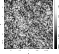
Figure 4: A Non-Gaussian simulation of the sky in real space obtained using the procedure described in Sec. 4.2.2

The maps simulated by drawing the pixel values from this pdf will be, by construction, statistically isotropic. They consist of non-Gaussian white noise with variance given by $\mu_{2}$. We then Fourier transform the map $\Delta T(\mn@boldsymbol{\hat{x}}_{p})$ to get the Fourier modes, $a(\mn@boldsymbol{u})$, which have variance proportional to $\mu_{2}$. We rescale these Fourier coefficients so that the variance is given by the correct angular power spectrum $C_{\ell}$. We then inverse Fourier transform these coefficients back to real space to produce a new signal map, $\Delta T(\mn@boldsymbol{\hat{x}}_{p})$, which now has the appropriate covariance matrix. In Fig. 4 we plot one of these non-Gaussian maps. This new map can then be used as input to simulate the VSA observational strategy and to obtain a set of visibilities as observed by the VSA. For our purposes we are interested in the simplest case, i.e. with no beam convolution and no noise, though these can easily be incorporated if we wish. We output the visibilities on a square grid, and then compute the bispectrum of these simulated visibilities with the same code that we apply to the real data.

By construction, the power spectrum of the non-Gaussian map is $C_{\ell}$ and the bispectrum is related to the skewness and variance of our non-Gaussian pdf by:

$$b_{\ell_{1}\ell_{2}\ell_{3}}=\frac{\mu_{3}}{\mu_{2}^{3/2}}A^{1/2}_{\mathrm{pix}}\sqrt{C_{\ell_{1}}C_{\ell_{2}}C_{\ell_{3}}}$$ (21)

where $A_{\mathrm{pix}}$ is the pixel area given by $A_{\mathrm{pix}}=L^{2}/N_{\mathrm{pix}}$, for a small patch of the sky of area $L^{2}$. For a detailed calculation see Rocha et al. (in preparation). In Fig. 5 we plot the computed values of the bispectrum against the predicted ones. The agreement shows that our bispectrum calculations are indeed correctly obtained.

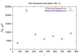
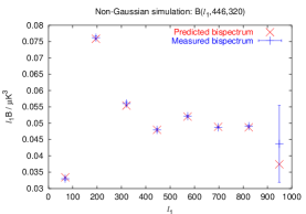
Figure 5: Bispectrum estimates of the non-Gaussian simulations with $\alpha_{1}=\alpha_{2}=0$, $\alpha_{3}=0.2$ and $\sigma_{0}=1$ (i.e. with $\mu_{3}\sim 0.95$ for a patch of the sky of side 28$\aas@@fstack{\circ}$6 and pixel number $N_{\mathrm{pix}}=128^{2}$), as compared to the predicted bispectrum obtained using equation (21). The error on the measured bispectrum are due to the finite number of simulations (1865).

We note that from the generalised Bayesian analysis using the non-Gaussian likelihood developed by Rocha et al. (2001), and applied to the VSA data by Savage et al. (2004), we concluded that VSA data are mostly consistent with zero $\alpha_{3}$, resulting in no evidence for this type of non-Gaussianity.

4.3 Testing for non-Gaussianity

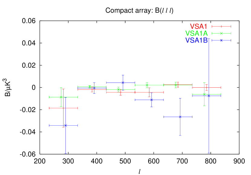
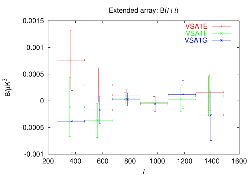
Figure 6: Estimated diagonal component of bispectrum from the compact (top) and extended (bottom) arrays for the region VSA1, with error bars from Gaussian simulations. Some values with very large errors at high and low $\ell$ have been omitted.

Fig. 6 shows the estimates of $B(\ell,\ell,\ell)$, together with error estimates from Gaussian simulations, from the observations of the three compact array fields and the three extended array fields in the VSA1 region. Little correlation can be seen between the three datasets in each graph. At low values of $\ell$ noisy estimates are obtained due to the fact that few triangles can be found at low $\ell$. The estimated variance of the mean is not dissimilar to the mean itself, indicating that we cannot expect to find a significant deviation from zero. The bispectrum estimates from the extended array are much less noisy than those from the compact array, reflecting the fact that the noise on the visibilities is smaller for the extended array than for the compact array (the mean noise per binned visibility is 4.4–8.8 Jy for the compact array and 0.7–1.1 Jy for the extended array). The noise contributes as $\sigma_{\mn@boldsymbol{u}}^{3}$ to the bispectrum error.

Figure 7: Results from simulations for VSA1 showing variance of bispectrum estimates and data values. The top figure shows the diagonal component of the bispectrum.

Figs 7 and 8 show a sample of the bispectrum values computed from the real data, together with the 1 and 2-$\sigma$ values from the Gaussian simulations. The change in the variance with multipole is due mainly to the variation in the number of triangles of vectors used to form each bispectrum estimate. In addition, the noise on each binned visibility value varies as a result of the differing numbers of raw visibility measurements used to form each binned value. The rough estimates of the errors from equation (15) agree well with the 1-$\sigma$ values from the simulations for large values of $\ell$, tending to be too small by approximately 0–4 per cent. However, for small values of $\ell$, equation (15) generally underestimates the variance by a greater amount, the most extreme example being for $B(366,366,366)$ where the estimated variance is only 35 per cent of the value obtained from simulations for the case of the VSA1F field. The distribution of this particular bispectrum value is very non-Gaussian, as shown in Fig. 9, and hence it appears that the correlations that we have neglected in equation (15) are significant in this case. Although around 160 different triangles of vectors in the $uv$ plane make up the bispectrum estimate, the effective number of independent triangles is much smaller.

For the 17 fields, there are a total of 1839 estimated bispectrum values. Of these, 99 were found to be greater than 2$\sigma$ in magnitude, compared with the expected value of $\sim$84 if the bispectrum estimates were Gaussian distributed (which we have found to be the case except for when one of the $\ell$s is small). The VSA3 field had a significant number of large bispectrum estimates (18 out of 176 of modulus $>2\sigma$, 6 of which were $>3\sigma$), most of the largest of which appear to have in common at least one value of $\ell$=584. There was one bispectrum estimate outside the 4-$\sigma$ limit, in the field VSA2G. In order to proceed further, we need a way of testing the data as a whole. In the following section we describe one such test that we have applied to the individual fields, as well as to sets of bispectrum estimates formed from the weighted sum of the estimates for individual fields that are in the same region of the sky.

Figure 8: Bispectrum estimates with variance from simulations for the extended array fields VSA1E and VSA1F.

Figure 9: Distribution of the bispectrum estimate $B(366,366,366)$ for the field VSA1F, and comparison with a Gaussian distribution with the same variance.

4.3.1 Kolmogorov-Smirnoff test

We wish to perform a quantitative comparison between our data and the simulations, in order to test the null hypothesis, $H_{0}$, that the data values were drawn from the same distribution as the Gaussian simulations. Following the method in Komatsu et al. (2002), for each bispectrum estimate $\hat{B}_{\alpha}$ we compute the quantity

$$P_{\alpha}=\frac{N\left(\left|\widehat{B}^{\mathrm{SIM}}_{\alpha}\right|<\left|\widehat{B}^{\mathrm{VSA}}_{\alpha}\right|\right)}{N_{\mathrm{Total}}},$$ (22)

where $\alpha$ represents a particular set of $\{\ell_{1},\ell_{2},\ell_{3}\}$ and $N_{\mathrm{Total}}=15000$, the total number of simulations. This gives the probability that the magnitude of the bispectrum estimate drawn under $H_{0}$ is less than the magnitude of the bispectrum estimate obtained from the data. If $H_{0}$ is true, then the distribution of $P_{\alpha}$ is uniform on the interval [0,1]. If there is a tendency towards a non-zero bispectrum we could (naïvely) expect to obtain more values of $P_{\alpha}$ close to 1. Fig. 10 shows the resulting cumulative distributions of $P_{\alpha}$ obtained for the VSA1 observations, in comparison with the straight line expected from a uniform distribution.

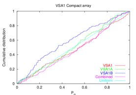
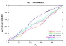
Figure 10: Cumulative distribution of $P_{\alpha}$ for the VSA1 compact and extended arrays.

The Kolmogorov-Smirnoff test operates by finding the quantity

$$D=\mathrm{max}\left|F_{e}(P)-F(P)\right|,$$ (23)

where $F_{e}$ is the empirical distribution function defined by

$$F_{e}(P)=\frac{N(P_{\alpha}<P)}{N},$$ (24)

and $F(P)$ is the continuous cumulative distribution function for $P$ under $H_{0}$. If the $P_{\alpha}$ are independent, identically distributed under $H_{0}$ then the distribution of $D$ is universal, depending only on the number of values, $N$.

Given $D=d$, one can then compute the tail probability $p$ which is given by

$$p(d)=\mathrm{Prob}(D\geq d\mid H_{0}).$$ (25)

In our case, we must calculate $p(d)$ using the distribution of $D$ obtained from simulations, since the assumption that the $P_{\alpha}$ are independent is invalid: although the formal covariance between different bispectrum estimates is zero apart for the effects of the primary beam, the same visibility point is used to calculate many different bispectrum estimates. Fig. 11 shows the distribution of $D$ obtained from simulations, compared with the distribution which would be obtained if the $P_{\alpha}$ were independently drawn from a uniform distribution. It can be seen that there is an increase of larger values of $D$. A very similar distribution is obtained from noise-only simulations, when there is no correlation between any of the visibility points.

Figure 11: The distribution of $D$ from simulations (solid line) as compared with the distribution obtained if the $P_{\alpha}$ were independent (dotted line), together with the measured value from the data for the field VSA3G.

Table 1 shows the calibrated results. It should be recognised that this test gives us an indication of how well the simulations match the data, which is dependent on a number of factors other than simply whether the data are Gaussian: whether the power spectrum is accurate and the correct telescope parameters have been used, and whether the noise estimate is correct. For comparison, when we compute the values of $P_{\alpha}$ by comparing the VSA1F data with Gaussian simulations which have a beam of FWHM 4$\aas@@fstack{\circ}$6 rather than 2$\aas@@fstack{\circ}$05, we obtain $p(d)=0.006$. Altering the amplitude of the power spectrum by $\sim$10 per cent was found to change only slightly the distribution of $d$, acting to alter $p(d)$ by $\sim$0.01.

Table 1: $d$-statistic and corresponding calibrated tail probability for the various fields. The number of bispectrum estimates for each field is $n$. The field labelled ‘VSA1 Compact’ represents the weighted average bispectrum from the individual VSA1 compact fields, and likewise for the others.

Field	$n$	$d$	$p(d)$
VSA1	171	0.076	0.38
VSA1A	106	0.064	0.81
VSA1B	106	0.16	0.03
VSA1 Compact	172	0.086	0.25
VSA1E	75	0.17	0.06
VSA1F	75	0.10	0.52
VSA1G	75	0.15	0.11
VSA1 Extended	75	0.11	0.34
VSA2	173	0.093	0.23
VSA2-OFF	174	0.084	0.29
VSA2 Compact	174	0.069	0.46
VSA2E	76	0.096	0.56
VSA2F	76	0.070	0.87
VSA2G	95	0.107	0.43
VSA2 Extended	95	0.103	0.43
VSA3	176	0.118	0.05
VSA3A	106	0.068	0.76
VSA3B	106	0.050	0.97
VSA3 Compact	176	0.084	0.23
VSA3E	97	0.107	0.45
VSA3F	76	0.090	0.62
VSA3G	76	0.176	0.05
VSA3 Extended	97	0.111	0.39

Four out of the 17 individual fields have values of $p(d)$ which are fairly low: VSA1B, VSA1E, VSA3 and VSA3G. For the total number of fields analysed we would expect an average of one to have $p(d)\leq 0.06$ by chance. The lowest value of $p(d)$ is for the VSA1B data, at 3 per cent. This field was observed for a total integration time of only 68 h, in comparison with around 200 hours for the majority of compact array fields (Taylor et al., 2003), and consequently the mean error on the visibilities is approximately twice that of the other fields. Furthermore, the large value of $d$ is caused by an excess of low values of $P_{\alpha}$, as can be seen in Fig. 10. This indicates that we should be very hesitant about drawing any conclusions about non-Gaussianity in the VSA1B field. The large value of $d$ for the VSA3G field is also due to an excess of low values of $P_{\alpha}$, whereas there is an excess of high values for the VSA3 and VSA1E fields. The VSA3 data have a greater extent in the $uv$ plane than the other two VSA3 compact array fields (hence the high value of $n$). On eliminating all the bispectrum values which are not calculated for the other two fields, we obtain $n=106$, $d=0.149$ and $p(d)=0.034$, so the significance level is increased slightly, indicating that the large bispectrum values are not concentrated in the region of large $\ell$. The VSA2 compact array fields, which have the longest integration times, are consistent with the simulations.

By testing the data in this way, we are making no assumptions about the type of non-Gaussianity that we are looking for. This means that our test is very general, but not very powerful as it is not tailored for optimal detection of any particular non-Gaussian signature. One disadvantage of the test is that all of the $P_{\alpha}$ values are given equal consideration, regardless of the fact that some bispectrum estimates are more dominated by noise than others. In the following section we consider two tests which are tailored for detecting particular types of non-Gaussianity: that arising from point sources, and from the time of recombination.

4.4 Point sources

4.4.1 Theory

A point source of strength $s$ at position $\mn@boldsymbol{x}_{0}$ can be described by

$$\Delta I(\mn@boldsymbol{\hat{x}})=s\,\delta(\mn@boldsymbol{\hat{x}}-\mn@boldsymbol{\hat{x}}_{0}).$$ (26)

The contribution this makes to the visibilities is

$$\Delta V(\mn@boldsymbol{u})=s\,A(\mn@boldsymbol{\hat{x}}_{0})\,e^{2\pi i{\mn@boldsymbol{\hat{x}}_{0}}.\mn@boldsymbol{u}},$$ (27)

and therefore the contribution to the bispectrum is

$$\Delta V(\mn@boldsymbol{u}_{1})\Delta V(\mn@boldsymbol{u}_{2})\Delta V(\mn@boldsymbol{u}_{3})\! =\! s^{3}\,A^{3}(\mn@boldsymbol{\hat{x}}_{0})\,e^{2\pi i{\mn@boldsymbol{\hat{x}}_{0}}.(\mn@boldsymbol{u}_{1}+\mn@boldsymbol{u}_{2}+\mn@boldsymbol{u}_{3})}$$ (28)

$$= s^{3}\,A^{3}(\mn@boldsymbol{\hat{x}}_{0}).$$

There will also be cross terms such as $V(\mn@boldsymbol{u}_{1})V(\mn@boldsymbol{u}_{2})\Delta V(\mn@boldsymbol{u}_{3})$ but these will have a mean value of zero. In addition, if we have several point sources there will be additional cross terms introduced. However, on average the contribution to the reduced bispectrum arising from point sources should be uniform (Komatsu & Spergel, 2001):

$$B^{\mathrm{ps}}(\ell_{1},\ell_{2},\ell_{3})=B^{\mathrm{ps}}.$$ (29)

So we can form an estimate of the point source contribution simply by calculating the (weighted) mean value of the bispectrum.

4.4.2 Point sources in the VSA data

We compared the estimated value of $B^{\mathrm{ps}}$ from the extended array data before and after source subtraction (Taylor et al., 2003; Grainge et al., 2003). The results are shown in Table 2, and illustrated in Fig. 12.

Table 2: Mean bispectrum values before and after point source subtraction for the three fields in the VSA1 region observed with the extended array.

Field	$\widehat{B}^{\mathrm{ps}}/(10^{-5}\mu\mathrm{K}^{3})$	$\widehat{B}^{\mathrm{ps}}/(10^{-5}\mu\mathrm{K}^{3})$	$\sigma/(10^{-5}\mu\mathrm{K}^{3})$
	Raw data	Sources subtracted
VSA1E	1.19	0.92	1.19
VSA1F	-0.96	-1.61	1.30
VSA1G	1.01	1.09	1.34

The mean value of the bispectrum is altered by $\sim$1–6$\times 10^{-6}\mu\mathrm{K}^{3}$ when the point sources are subtracted. Therefore, although subtracting the sources does change the bispectrum estimates, the resulting difference is considerably smaller than the standard deviation on the mean value of the bispectrum which arises from sample variance and noise, and so it does not seem possible to detect point sources in this way. However, if future VSA observations have a much lower noise and probe higher values of $\ell$ then it may be possible to use the bispectrum to detect the presence of point sources.

Figure 12: Diagonal component of the bispectrum for the fields VSA1E and VSA1F before and after point source subtraction, illustrating the level of change.

4.4.3 Residual point sources

We can estimate the contribution to the bispectrum from residual point sources using the results of the 15-GHz Ryle survey (Waldram et al., 2003). This survey found that the differential source count at 15 GHz could be well approximated by

$$n(S)\approx K\left(\frac{S}{\mathrm{Jy}}\right)^{-\beta}\mathrm{Jy^{-1}sr^{-1}},$$ (30)

where $S$ is the flux density, $\beta=2.15$ and $K=51$. Assuming a spectral index $\alpha=0.55$ we find that, at 34 GHz, $K=30$.

An individual point source contributes to the three-point visibility function as described by equation (28). Assuming a Poisson distribution of sources, the mean contribution from unsubtracted sources can be expressed as

$$\langle V(\mn@boldsymbol{u}_{1})V(\mn@boldsymbol{u}_{2})V(\mn@boldsymbol{u}_{3})\rangle = \int A^{3}(\mn@boldsymbol{\hat{x}})\;d^{2}\mn@boldsymbol{\hat{x}}\int_{0}^{S_{*}}S^{3}n(S)\;dS$$ (31)

$$= \frac{2}{3}\pi\sigma^{2}K\frac{S_{*}^{4-\beta}}{4-\beta},$$

for $\mn@boldsymbol{u}_{1}+\mn@boldsymbol{u}_{2}+\mn@boldsymbol{u}_{3}=0$, where $S_{*}$ is the source subtraction level.

For the compact array, taking $S_{*}$ = 80 mJy we obtain a theoretical contribution from unsubtracted sources of $\sim 4\times 10^{-4}\mathrm{Jy^{3}}$ (equivalent to $4\times 10^{-6}\mu\mathrm{K}^{3}$) and for the extended array, taking $S_{*}$ = 20 mJy we obtain $\sim 6\times 10^{-6}\mathrm{Jy^{3}}$ (equivalent to $3\times 10^{-7}\mu\mathrm{K}^{3}$). Comparing this with the error on the mean value of the bispectrum of $\sim 10^{-4}\mu\mathrm{K^{3}}$ for the compact array and $\sim 10^{-5}\mu\mathrm{K^{3}}$ for the extended array, we see that we do not expect the bispectrum to detect the presence of the residual sources.

If we take these values and consider the comparison with the predicted bispectrum arising from the coupling between the Sunyaev-Zel’dovich effect and weak lensing effects, as given by Komatsu & Spergel (2001), we find that the SZ-lensing bispectrum will be overwhelmed by residual point sources at the source subtraction level of the extended array for $\ell\gtrsim 200$. At lower values of $\ell$ we estimate that the SZ-lensing contribution to the bispectrum is approximately four orders of magnitude smaller than the error on our bispectrum estimates. Therefore our data is not sensitive to this effect.

4.5 Simulated point sources

4.5.1 Noise-only simulations

As a preliminary test we subtracted a single point source from an extended-array simulation with no noise or CMB signal. The resulting mean bispectrum was 96 per cent of the theoretical value of $s^{3}A^{3}(\mn@boldsymbol{\hat{x}}_{0})$, with all the individual bispectrum estimates being very similar in value. The discrepancy is due to the fact that we slightly relax the requirement that $\mn@boldsymbol{u}_{1}+\mn@boldsymbol{u}_{2}+\mn@boldsymbol{u}_{3}=0$ and so the phase in equation (28) is slightly non-zero.

On subtracting two point sources (of flux density 1.0 Jy and 0.89 Jy after attenuation) from the same simulation, we immediately find that each individual bispectrum estimate is very different, varying from -0.048 Jy³ to -2.4 Jy³, as a result of the cross-terms. The mean bispectrum value is -1.3 Jy³ compared to a theoretical value of -1.7 Jy³. On subtracting the VSA1E source list, 10 sources in total, the mean bispectrum value is -2.95$\times 10^{-5}\mathrm{Jy}^{3}$ in comparison with the theoretical value of -3.53$\times 10^{-5}\mathrm{Jy}^{3}$, and there is less variation between individual bispectrum estimates, suggesting that with more sources the cross-terms have a greater tendency to cancel.

In order to ascertain the effect of noise on our ability to detect point sources we used sets of simulated data with no CMB component, just noise, to which we added the point sources subtracted from the VSA1E field. Each simulation had exactly the same $uv$ and noise template apart from an overall scaling factor on the noises. The values of the mean bispectra, together with the standard deviation of the mean bispectrum obtained from noise-only simulations, are shown in Table 3.

Table 3: The rms noise, mean bispectrum values and standard deviations for noise-only simulations with point sources added.

rms noise / Jy	$\langle B\rangle/10^{-5}\mbox{Jy}^{3}$	$\sigma/10^{-5}\mbox{Jy}^{3}$
	[/$10^{-5}\mu\mathrm{K}^{3}$]	[/$10^{-5}\mu\mathrm{K}^{3}$]
2.2	8.8 [4.4]	390 [19]
0.44	3.59 [0.18]	3.1 [0.15]
0.22	1.89 [0.093]	0.39 [0.019]
0.044	2.13 [0.11]	3.1$\times 10^{-3}$ [1.5$\times 10^{-4}$]
0.0044	2.22 [0.11]	3.1$\times 10^{-6}$ [1.5$\times 10^{-7}$]

Figure 13: Bispectrum estimates from noise-only simulations with point sources added, with theoretical bispectrum plotted as a horizontal line. $\alpha$ represents a particular set of $\{\ell_{1},\ell_{2},\ell_{3}\}$

The mean value of the bispectrum is positive in all cases, but a definite detection of point sources is obtained only when the rms noise is less than 0.44 Jy. The point source bispectrum is completely swamped by noise for the case with the highest noise. Fig. 13 illustrates the bispectrum components for each case.

There were 10 sources in the simulations in total, and the sum $\sum_{i=1}^{10}A^{3}(\mn@boldsymbol{\hat{x}}_{i})s_{i}^{3}$ is $3.5\times 10^{-5}\mbox{Jy}^{3}$. This is 1.6 times the mean bispectrum value calculated, weighting according to the variance from simulations. However, if we use an alternative weighting scheme, according to the number of triangles of vectors which are combined to form each bispectrum estimate, we obtain (for the lowest noise case) a mean bispectrum value of $2.6\times 10^{-5}\mbox{Jy}^{3}$. The cross-terms introduce a lot of variation between the different individual bispectrum estimates and hence cause the final values to depend on the weighting scheme.

The rms noise on each visibility point for the VSA1E data is $\sim$1 Jy, which is at a level at which the contribution from point sources is swamped by noise. In addition, the CMB itself will increase further the variance on the mean value of the bispectrum. Therefore we cannot expect that we will detect the presence of sources in the extended array data using this method.

For comparison, we also performed the Kolmogorov-Smirnoff test on the point source simulations. This gave a conclusive detection of non-Gaussianity for the cases with a rms of 0.0044 Jy and 0.044 Jy but no detection when the rms noise was 0.22 Jy [the value of $p(d)$ was 0.42] despite the conclusive detection found by computing the mean value of the bispectrum. This illustrates how using a tailored statistic when searching for a particular non-Gaussian signal is a much more powerful method of detection than using a general statistic.

4.5.2 CMB simulation with strong sources

We computed the mean bispectrum from a simulation based on the noise and $uv$-positions of an extended-array field, with both CMB and bright sources. The observed sky is shown in Fig. 14 with the point sources clearly visible in the map. The mean bispectrum value was $0.3$ Jy³, a factor of 1000 greater than the standard deviation from simulations with no point sources. The bispectrum is sensitive to the point sources as (source strength)³ and so is useful for detecting strong sources but not for weak sources.

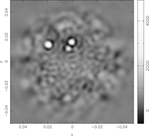
Figure 14: Simulated CMB with point sources, convolved with the primary beam.

4.6 Primordial Non-Gaussianity

It has become usual to quantify the primordial non-Gaussianity which arises from weak non-linear evolution on super-Hubble scales by a single parameter $f_{\mathrm{NL}}$, the non-linear coupling parameter:

$$\mathcal{R}(\mn@boldsymbol{x})=\mathcal{R}_{G}(\mn@boldsymbol{x})+f_{\mathrm{NL}}(\mathcal{R}_{G}^{2}(\mn@boldsymbol{x})-\langle\mathcal{R}_{G}^{2}(\mn@boldsymbol{x})\rangle),$$ (32)

where $\mathcal{R}(\mn@boldsymbol{x})$ is the comoving curvature perturbation as defined according to the convention in Liddle & Lyth (2000), and $\mathcal{R}_{G}(\mn@boldsymbol{x})$ its Gaussian component (Acquaviva et al., 2003; Maldacena, 2003). Even if the fluctuations produced by inflation are perfectly Gaussian, a non-zero $f_{\mathrm{NL}}$ will be at second-order in perturbation theory due to the non-linear nature of general relativity (Bartolo et al., 2004). The current distribution of matter, which is highly non-Gaussian, is a result of the non-perturbative non-linear coupling between modes, which becomes increasingly significant after recombination as the perturbations grow. Previous studies have not detected any significant primordial non-Gaussianity, but have simply put upper limits on it. This is not surprising as the predictions from all but the most contrived inflationary models are well below the current upper limits. The recent results from WMAP place an upper limit of 89 on the value of $f_{\mathrm{NL}}$ (Komatsu et al., 2003), in comparison with predictions from slow-roll inflation which give $\left|f_{\mathrm{NL}}\right|\sim 10^{-1}$–$10^{-2}$, apart from the non-Gaussianity introduced by the subsequent evolution of the perturbations.

We should therefore only expect to place limits on the value of $f_{\mathrm{NL}}$ using the VSA data, but it is interesting to see what limits the data are capable of producing. In addition, the techniques developed to estimate $f_{\mathrm{NL}}$ can easily be applied to any other theoretical bispectrum which has its amplitude as the only free parameter.

We calculated the theoretical bispectrum for the case $f_{\mathrm{NL}}$=1 using a modified version of CAMB (Lewis, Challinor & Lasenby, 2000). The resulting bispectrum has features on the usual acoustic scale of the power spectrum, and its diagonal component is shown in Fig. 15.

Figure 15: Diagonal component of the theoretical bispectrum for $f_{\mathrm{NL}}=1$.

In order to relate the theoretical bispectrum to the measured three-point visibility function, we performed the integral described in Appendix C which convolves the bispectrum with the aperture function. For each field, we then estimate the set of $Q_{\alpha}$, the theoretical values of the $B_{\alpha}$ for $f_{\mathrm{NL}}=1$ [where $\alpha=(\ell_{1},\ell_{2},\ell_{3})$] according to equation (13) using the predicted value of $\langle S(\mn@boldsymbol{u}_{1})S(\mn@boldsymbol{u}_{2})S(\mn@boldsymbol{u}_{3})\rangle$ as calculated from the integral. Figure 16 shows the resulting diagonal component of the theoretical measured bispectrum.

Figure 16: Diagonal component of theoretical measured bispectrum for the VSA2 data with $f_{\mathrm{NL}}=1$

We estimate the value of $f_{\mathrm{NL}}$ from our bispectrum estimates with the estimator

$$\widehat{f}_{\mathrm{NL}}=\frac{\sum_{\alpha}\frac{\hat{B}_{\alpha}Q_{\alpha}}{\sigma^{2}_{\alpha}}}{\sum_{\beta}\frac{Q^{2}_{\beta}}{\sigma^{2}_{\beta}}},$$ (33)

where the $\sigma^{2}_{\alpha}$ are the variances of the bispectrum estimates from Gaussian simulations. We obtain these variances from mosaiced simulations to allow us properly to include mosaiced fields. Equation (33) reduces to the optimal linear estimator of $f_{\mathrm{NL}}$ from the bispectrum estimates in the limit that these are uncorrelated.

The overall estimate of $f_{\mathrm{NL}}$ obtained from the compact array data is 85, with a standard deviation of 2700. For the extended array, we obtain an estimate of -400 with a standard deviation of 3500. The 95 per cent confidence limits are 5400 and 7000 for the compact and extended arrays respectively. These contraints are slightly weaker than those obtained from the MAXIMA data using the FFT estimator (Santos et al., 2003), due probably to the fact that the MAXIMA data extend to lower multipoles with slightly higher $\Delta\ell$ resolution, although the VSA sky coverage is slightly greater. [The VSA compact array data cover 101 deg² (Taylor et al., 2003); the MAXIMA data used had an area of 60 deg².] This is also why the compact array data are better at constraining $f_{\mathrm{NL}}$ than the extended array data. The bispectrum arising from primordial non-Gaussianity falls quickly with $\ell$ and so extending the measurements to higher values of $\ell$ does not significantly improve the constraints (unless the noise is very low). This is why the WMAP data, which are cosmic-variance limited at low $\ell$, are able to place so much tighter constraints on $f_{\mathrm{NL}}$.

5 Conclusions

Our bispectrum calculations indicate a slightly greater discrepancy with the Gaussian simulations for the fields VSA1B, VSA1E, VSA3, and VSA3G than we would expect if the CMB sky were perfectly Gaussian. However, there is little discernible pattern in the way in which the data deviate from the simulations. A small level of non-Gaussianity is to be expected as there will inevitably be a degree of foreground contamination and unsubtracted point sources, but we have shown that in the case of point sources we do not anticipate to be able to detect the resulting non-Gaussianity with the current level of experimental noise. In the case of point sources, the CMB itself acts as a level of noise that can only be reduced by taking measurements at higher $\ell$. We note that Savage et al. (2004) found some evidence for non-Gaussianity in the VSA1 mosaic, which was attributed to point sources or contamination from galactic foregrounds. It is possible that the excess of large bispectrum values in the VSA1E field arises from the same cause. The fact the low values of the tail probability $p(d)$ in a Kolmogorov-Smirnoff test only appear in isolated individual fields indicate that, if the non-Gaussianity which is hinted at is real, it is localised in space.

The limit on the largest scales probed by the VSA means that it can only be used to place weak constraints on the value of the quadratic non-Gaussianity parameter $f_{\mathrm{NL}}$. The data are more suited to detecting non-Gaussianity that is present on smaller scales.

Appendix A Optimal cubic bispectrum estimators

We have estimated the bispectrum using a simple cubic estimator with each visibility weighted by the inverse of its variance (see equation 13). This estimator is not optimal, but for interferometer data, where the signal and noise covariances are nearly diagonal, it is close to optimal as we shall argue in this appendix.

We begin by reviewing the calculation of the optimal cubic estimator, first given by Heavens (1998) and discussed further by Santos et al. (2003). For simplicity, consider real data $\{a_{i}\}$ whose three-point function is related to the bispectrum $B_{\alpha}$ that we wish to estimate by

$$\langle a_{i}a_{j}a_{k}\rangle=\sum_{\alpha}Q^{\alpha}_{ijk}B_{\alpha}.$$ (34)

Here, $\alpha$ denotes an (ordered) triplet $\ell_{1}\geq\ell_{2}\geq\ell_{3}$ and $Q^{\alpha}_{ijk}$ is totally symmetric in $i$, $j$ and $k$. We construct an estimator $\hat{y}_{\alpha}$ which is cubic in the $\{a_{i}\}$,

$$\hat{y}_{\alpha}=\sum_{ijk}E^{\alpha}_{ijk}a_{i}a_{j}a_{k},$$ (35)

and which is unbiased,

$$\langle\hat{y}_{\alpha}\rangle=\sum_{ijk}E^{\alpha}_{ijk}\sum_{\beta}Q^{\beta}_{ijk}B_{\beta}\quad\Rightarrow\quad\sum_{ijk}E^{\alpha}_{ijk}Q^{\beta}_{ijk}=\delta_{\alpha\beta}.$$ (36)

Only the symmeterised part of $E^{\alpha}_{ijk}$ enters the estimator $\hat{y}_{\alpha}$ but we do not impose total symmetry at this stage as enforcing this complicates the variational procedure that follows. Following Heavens (1998), we construct the variance of $\hat{y}_{\alpha}$ under the assumption that the data are Gaussian (so the estimator is optimised for only weakly non-Gaussian data), to find

$$\mathrm{var}(\hat{y}_{\alpha})=\sum_{ijk}\sum_{i^{\prime}j^{\prime}k^{\prime}}E^{\alpha}_{ijk}E^{\alpha}_{i^{\prime}j^{\prime}k^{\prime}}(C_{ii^{\prime}}C_{jj^{\prime}}C_{kk^{\prime}}+\mathrm{perms}),$$ (37)

where $C_{ij}\equiv\langle a_{i}a_{j}\rangle$ is the (symmetric) covariance of the data. Unlike Heavens (1998), we have not imposed symmetry of $E^{\alpha}_{ijk}$, so we cannot simplify equation (37) in the manner that he does (see his equation 16). We now vary $E^{\alpha}_{ijk}$ to minimise the variance of $\hat{y}_{\alpha}$, enforcing the constraints on the mean (equation 36) with a set of Lagrange multipliers $\lambda_{\alpha\beta}$, to find

$$6\sum_{ijk}E^{\alpha}_{(ijk)}(2C_{ii^{\prime}}C_{jj^{\prime}}C_{kk^{\prime}}+3C_{ij}C_{k(i^{\prime}}C_{j^{\prime}k^{\prime})})-\sum_{\beta}\lambda_{\alpha\beta}Q^{\beta}_{i^{\prime}j^{\prime}k^{\prime}}=0.$$ (38)

Note that only the symmetric part $E^{\alpha}_{(ijk)}$ enters this expression and so only that part is constrained as expected. We can now solve for a symmetric $E^{\alpha}_{ijk}$ and $\lambda_{\alpha\beta}$ to find

$$E^{\alpha}_{ijk}=\sum_{\beta}\lambda_{\alpha\beta}\sum_{i^{\prime}j^{\prime}k^{\prime}}Q^{\beta}_{i^{\prime}j^{\prime}k^{\prime}}\left(\frac{1}{12}C^{-1}_{ii^{\prime}}C^{-1}_{jj^{\prime}}C^{-1}_{kk^{\prime}}-\frac{1}{4(4+N)}C^{-1}_{i^{\prime}j^{\prime}}C^{-1}_{k^{\prime}(i}C^{-1}_{jk)}\right)$$ (39)

where

$$\lambda^{-1}_{\alpha\beta}=\frac{1}{12}\sum_{ijk}\sum_{i^{\prime}j^{\prime}k^{\prime}}Q^{\alpha}_{ijk}Q^{\beta}_{i^{\prime}j^{\prime}k^{\prime}}\left(C^{-1}_{ii^{\prime}}C^{-1}_{jj^{\prime}}C^{-1}_{kk^{\prime}}-\frac{3}{4+N}C^{-1}_{i^{\prime}j^{\prime}}C^{-1}_{k^{\prime}i}C^{-1}_{jk}\right).$$ (40)

In these expressions, $N$ is the number of data points and is typically very large. Our equations (39) and (40) correct the results given as equations (21) and (25) in Heavens (1998). The error in the latter analysis arises because symmetry of $E^{\alpha}_{ijk}$ is assumed prior to the variation, but is then not enforced during it. However, the terms in error in Heavens (1998) are suppressed by $1/N$ for large $N$, and so the differences from the results derived here are small for $N\gg 1$.

For interferometer data, the covariance matrix $C_{ij}$ is close to diagonal with correlations limited roughly to the extent of the aperture function. Multiplication by $C^{-1}_{ij}$ reduces to inverse variance weighting the visibilities if the effect of the primary beam is neglected. Furthermore, in this limit $Q^{\alpha}_{ijk}$ enforces $\mn@boldsymbol{u}_{i}+\mn@boldsymbol{u}_{j}+\mn@boldsymbol{u}_{k}=0$, so that equation (39), with $N\gg 1$, reduces to the heuristically-weighted estimator of equation (13). In practice, the finite extent of the primary beam makes the heuristic estimator somewhat sub-optimal. The necessary developments to compute the optimal estimator are given in Appendix C, where we construct $Q^{\alpha}_{ijk}$. However, given the need to perform large-volume Monte-Carlo simulations to assess properly the significance of our results, employing the optimal estimator would have been prohibitively slow for the analysis in this paper.

Appendix B Interferometer measurements

The actual values recorded by the VSA are flux density measurements in Janskys. The receivers are calibrated primarily by observations of Jupiter (Taylor et al., 2003), with the primary beam $A(\mn@boldsymbol{x})$ normalised so that $A(0)=1$. The intensity fluctuations of the CMB can be connected to the temperature fluctuations by

$$\Delta I(\mn@boldsymbol{\hat{x}},\nu)\approx\frac{\partial B(\nu,T)}{\partial T}\Big{|}_{T=T_{0}}\Delta T_{\mathrm{cmb}}(\mn@boldsymbol{\hat{x}}).$$ (41)

The visibility seen by the interferometer can be expressed as

$$S(\mn@boldsymbol{u})=\int\Delta I(\mn@boldsymbol{\hat{x}})\;A(\mn@boldsymbol{\hat{x}})\>e^{2\pi i\mn@boldsymbol{u.\hat{x}}}\>\mathrm{d^{2}}\mn@boldsymbol{\hat{x}}.$$ (42)

The measured visibility $V(\mn@boldsymbol{\hat{u}})$ is related to this by

$$V(\mn@boldsymbol{u})=S(\mn@boldsymbol{u})+N(\mn@boldsymbol{u}),$$ (43)

where $N(\mn@boldsymbol{u})$ is the noise on baseline $\mn@boldsymbol{u}$. We can relate this to the values of $a(\mn@boldsymbol{u})$ by

$$S(\mn@boldsymbol{u}) = \frac{\partial B(\nu,T)}{\partial T}\Big{|}_{T=T_{0}}T_{0}\ a(\mn@boldsymbol{u})\star\tilde{A}(\mn@boldsymbol{u})$$ (44)

$$= fa(\mn@boldsymbol{u})\star\tilde{A}(\mn@boldsymbol{u})$$ (45)

where $f=94\times 10^{6}\mathrm{Jy\>sr^{-1}}$ for $\nu$ = 34 GHz and a CMB temperature $T_{0}$ of 2.726K (Mather et al., 1994). If we consider the variance of the measured signal we obtain

$$\left\langle V(\mn@boldsymbol{u})V^{\ast}(\mn@boldsymbol{u})\right\rangle = f^{2}\int\!\mathrm{d^{2}}\mn@boldsymbol{u}_{1}\int\!\mathrm{d^{2}}\mn@boldsymbol{u}_{2}\>\tilde{A}(\mn@boldsymbol{u}\!-\!\mn@boldsymbol{u}_{1})\tilde{A}^{\ast}(\mn@boldsymbol{u}\!-\!\mn@boldsymbol{u}_{2})\left\langle a(\mn@boldsymbol{u}_{1})a^{\ast}(\mn@boldsymbol{u}_{2})\right\rangle+\sigma^{2}_{\mn@boldsymbol{u}}$$

$$= f^{2}\int\!\mathrm{d^{2}}\mn@boldsymbol{u}_{1}\int\!\mathrm{d^{2}}\mn@boldsymbol{u}_{2}\>C(u_{1})\delta(\mn@boldsymbol{u}_{1}-\mn@boldsymbol{u}_{2})\tilde{A}(\mn@boldsymbol{u}\!-\!\mn@boldsymbol{u}_{1})\tilde{A}^{\ast}(\mn@boldsymbol{u}\!-\!\mn@boldsymbol{u}_{2})+\sigma^{2}_{\mn@boldsymbol{u}}$$

$$\approx f^{2}C(u)\int\mathrm{d}^{2}\mn@boldsymbol{u}_{1}\left|A(\mn@boldsymbol{u}_{1})\right|^{2}+\sigma^{2}_{\mn@boldsymbol{u}},$$

if we make the approximation that $C(u)$ is constant over the width of the aperture function. (We use $u_{i}$ to denote $|\mn@boldsymbol{u}_{i}|$.) Here, $\sigma^{2}_{\mn@boldsymbol{u}}$ is the variance of the noise, which is statistically independent of the visibility measurement.

If $A(\mn@boldsymbol{x})=\exp({-|\mn@boldsymbol{x}|^{2}/2\sigma^{2}})$ then we find that

$$\left\langle V(\mn@boldsymbol{u})V^{\ast}(\mn@boldsymbol{u})\right\rangle\approx\pi\sigma^{2}f^{2}C(u)+\sigma^{2}_{\mn@boldsymbol{u}}.$$ (46)

Similarly, if we consider

$$\left\langle V(\mn@boldsymbol{u}_{1})V(\mn@boldsymbol{u}_{2})V(\mn@boldsymbol{u}_{3})\right\rangle = f^{3}\int\!\mathrm{d^{2}}\mn@boldsymbol{u}_{1}^{\prime}\int\!\mathrm{d^{2}}\mn@boldsymbol{u}_{2}^{\prime}\int\!\mathrm{d^{2}}\mn@boldsymbol{u}_{3}^{\prime}\tilde{A}(\mn@boldsymbol{u}_{1}\!-\!\mn@boldsymbol{u}_{1}^{\prime})\tilde{A}(\mn@boldsymbol{u}_{2}\!-\!\mn@boldsymbol{u}_{2}^{\prime})\tilde{A}(\mn@boldsymbol{u}_{3}\!-\!\mn@boldsymbol{u}_{3}^{\prime})B(u_{1}^{\prime},u_{2}^{\prime},u_{3}^{\prime})\delta^{2}(\mn@boldsymbol{u}_{1}^{\prime}+\mn@boldsymbol{u}_{2}^{\prime}+\mn@boldsymbol{u}_{3}^{\prime})$$ (47)

$$\approx f^{3}B(u_{1},u_{2},u_{3})\int\!\mathrm{d^{2}}\mn@boldsymbol{\hat{x}}\int\!\mathrm{d^{2}}\mn@boldsymbol{u}_{1}^{\prime}\int\!\mathrm{d^{2}}\mn@boldsymbol{u}_{2}^{\prime}\int\!\mathrm{d^{2}}\mn@boldsymbol{u}_{3}^{\prime}$$

$$\times\exp[2\pi i\mn@boldsymbol{\hat{x}}.(\mn@boldsymbol{u}_{1}^{\prime}+\mn@boldsymbol{u}_{2}^{\prime}+\mn@boldsymbol{u}_{3}^{\prime})]\tilde{A}(\mn@boldsymbol{u}_{1}\!-\!\mn@boldsymbol{u}_{1}^{\prime})\tilde{A}(\mn@boldsymbol{u}_{2}\!-\!\mn@boldsymbol{u}_{2}^{\prime})\tilde{A}(\mn@boldsymbol{u}_{3}\!-\!\mn@boldsymbol{u}_{3}^{\prime})$$

$$= f^{3}B(u_{1},u_{2},u_{3})\int\!\mathrm{d^{2}}\mn@boldsymbol{x}A^{3}(\mn@boldsymbol{\hat{x}})\exp[2\pi i\mn@boldsymbol{\hat{x}}.(\mn@boldsymbol{u}_{1}+\mn@boldsymbol{u}_{2}+\mn@boldsymbol{u}_{3})],$$

assuming that the bispectrum varies only slowly over the width of the aperture function, and that the noise is Gaussian. Taking the above form for $A(\mn@boldsymbol{x})$ and the case $\mn@boldsymbol{u}_{1}+\mn@boldsymbol{u}_{2}+\mn@boldsymbol{u}_{3}=0$ we obtain

$$\left\langle V(\mn@boldsymbol{u}_{1})V(\mn@boldsymbol{u}_{2})V(\mn@boldsymbol{u}_{3})\right\rangle\approx f^{3}\frac{2}{3}\pi\sigma^{2}B(u_{1},u_{2},u_{3}).$$ (48)

Appendix C Visibility three-point function

In this appendix we derive an integral expression for the three-point function of the interferometer visibilities. For the special case of a Gaussian beam, we are able to reduce the integral further to obtain a closed-form expression for the quantity $Q^{\alpha}_{ijk}$ introduced in Appendix A.

Our starting point is the first equality in equation (47) which expresses the three-point function of the visibilities as an integral over the bispectrum:

$$\langle S(\mn@boldsymbol{u}_{1})S(\mn@boldsymbol{u}_{2})S(\mn@boldsymbol{u}_{3})\rangle=\int_{-\infty}^{\infty}\mathrm{d}^{2}\mn@boldsymbol{u}_{1}^{\prime}\int_{-\infty}^{\infty}\mathrm{d}^{2}\mn@boldsymbol{u}_{2}^{\prime}\int_{-\infty}^{\infty}\mathrm{d}^{2}\mn@boldsymbol{u}_{3}^{\prime}B(u_{1}^{\prime},u_{2}^{\prime},u_{3}^{\prime})\tilde{A}(\mn@boldsymbol{u}_{1}-\mn@boldsymbol{u}_{1}^{\prime})\tilde{A}(\mn@boldsymbol{u}_{2}-\mn@boldsymbol{u}_{2}^{\prime})\tilde{A}(\mn@boldsymbol{u}_{3}-\mn@boldsymbol{u}_{3}^{\prime})\delta^{2}(\mn@boldsymbol{u}_{1}^{\prime}+\mn@boldsymbol{u}_{2}^{\prime}+\mn@boldsymbol{u}_{3}^{\prime}).$$ (49)

We can divide the region of integration into six separate regions, $u_{1}^{\prime}\geq u_{2}^{\prime}\geq u_{3}^{\prime}$ and its permutations. Since $B(u_{1}^{\prime},u_{2}^{\prime},u_{3}^{\prime})$ is invariant under permutations of the $\mn@boldsymbol{u}_{i}^{\prime}$, as is $\delta^{2}(\mn@boldsymbol{u}_{1}^{\prime}+\mn@boldsymbol{u}_{2}^{\prime}+\mn@boldsymbol{u}_{3}^{\prime})$, we can permute the $\mn@boldsymbol{u}_{i}$ instead of the $\mn@boldsymbol{u}_{i}^{\prime}$ to find

$$\langle S(\mn@boldsymbol{u}_{1})S(\mn@boldsymbol{u}_{2})S(\mn@boldsymbol{u}_{3})\rangle=\int_{u_{1}^{\prime}\geq u_{2}^{\prime}\geq u_{3}^{\prime}}\mathrm{d}^{2}\mn@boldsymbol{u}_{1}^{\prime}\mathrm{d}^{2}\mn@boldsymbol{u}_{2}^{\prime}\mathrm{d}^{2}\mn@boldsymbol{u}_{3}^{\prime}B(u_{1}^{\prime},u_{2}^{\prime},u_{3}^{\prime})\sum_{\stackrel{{\scriptstyle\mathrm{perms}}}{{\{\mn@boldsymbol{u}_{1},\mn@boldsymbol{u}_{2},\mn@boldsymbol{u}_{3}\}}}}\tilde{A}(\mn@boldsymbol{u}_{1}-\mn@boldsymbol{u}_{1}^{\prime})\tilde{A}(\mn@boldsymbol{u}_{2}-\mn@boldsymbol{u}_{2}^{\prime})\tilde{A}(\mn@boldsymbol{u}_{3}-\mn@boldsymbol{u}_{3}^{\prime})\delta^{2}(\mn@boldsymbol{u}_{1}^{\prime}+\mn@boldsymbol{u}_{2}^{\prime}+\mn@boldsymbol{u}_{3}^{\prime}).$$ (50)

Transforming to polar coordinates, the delta function restricts the lower bounds of $u_{2}^{\prime}$ and $u_{3}^{\prime}$ by the triangle inequality, hence

$$\langle S(\mn@boldsymbol{u}_{1})S(\mn@boldsymbol{u}_{2})S(\mn@boldsymbol{u}_{3})\rangle = \int_{0}^{\infty}u_{1}^{\prime}\mathrm{d}u_{1}^{\prime}\int_{u_{1}^{\prime}/2}^{u_{1}^{\prime}}u_{2}^{\prime}\mathrm{d}u_{2}^{\prime}\int_{u_{1}^{\prime}-u_{2}^{\prime}}^{u_{2}^{\prime}}u_{3}^{\prime}\mathrm{d}u_{3}^{\prime}B(u_{1}^{\prime},u_{2}^{\prime},u_{3}^{\prime})$$ (51)

$$\mbox{}\left(\int_{0}^{2\pi}\mathrm{d}\phi_{1}^{\prime}\int_{0}^{2\pi}\mathrm{d}\phi_{2}^{\prime}\int_{0}^{2\pi}\mathrm{d}\phi_{3}^{\prime}\sum_{\stackrel{{\scriptstyle\mathrm{perms}}}{{\{\mn@boldsymbol{u}_{1},\mn@boldsymbol{u}_{2},\mn@boldsymbol{u}_{3}\}}}}\tilde{A}(\mn@boldsymbol{u}_{1}-\mn@boldsymbol{u}_{1}^{\prime})\tilde{A}(\mn@boldsymbol{u}_{2}-\mn@boldsymbol{u}_{2}^{\prime})\tilde{A}(\mn@boldsymbol{u}_{3}-\mn@boldsymbol{u}_{3}^{\prime})\delta^{2}(\mn@boldsymbol{u}_{1}^{\prime}+\mn@boldsymbol{u}_{2}^{\prime}+\mn@boldsymbol{u}_{3}^{\prime})\right).$$

For every $u_{1}^{\prime}$, $u_{2}^{\prime}$ and $u_{3}^{\prime}$ within the domain of integration, the delta function fixes $\phi_{2}^{\prime}=\phi_{1}^{\prime}+\psi$, where the two values of $\psi\in[-\pi/2,\pi/2]$ are given by the cosine rule $2u_{1}^{\prime}u_{2}^{\prime}\cos\psi=u_{3}^{\prime}{}^{2}-u_{2}^{\prime}{}^{2}-u_{1}^{\prime}{}^{2}$, and $\phi_{3}^{\prime}=\phi_{\mn@boldsymbol{u}_{1}^{\prime}+\mn@boldsymbol{u}_{2}^{\prime}}+\pi$ closes the triangle. Performing the (trivial) integrations over $\phi_{2}^{\prime}$ and $\phi_{3}^{\prime}$, we find that

$$\langle S(\mn@boldsymbol{u}_{1})S(\mn@boldsymbol{u}_{2})S(\mn@boldsymbol{u}_{3})\rangle = \int_{0}^{\infty}u_{1}^{\prime}\mathrm{d}u_{1}^{\prime}\int_{u_{1}^{\prime}/2}^{u_{1}^{\prime}}u_{2}^{\prime}\mathrm{d}u_{2}^{\prime}\int_{u_{1}^{\prime}-u_{2}^{\prime}}^{u_{2}^{\prime}}u_{3}^{\prime}\mathrm{d}u_{3}^{\prime}\frac{2B(u_{1}^{\prime},u_{2}^{\prime},u_{3}^{\prime})}{\sqrt{4u_{1}^{\prime}{}^{2}u_{2}^{\prime}{}^{2}-(u_{3}^{\prime}{}^{2}-u_{1}^{\prime}{}^{2}-u_{2}^{\prime}{}^{2})^{2}}}$$ (52)

$$\mbox{}\left(\int_{0}^{2\pi}\mathrm{d}\phi_{1}^{\prime}\sum_{\stackrel{{\scriptstyle\mathrm{perms}}}{{\{\mn@boldsymbol{u}_{1},\mn@boldsymbol{u}_{2},\mn@boldsymbol{u}_{3}\}}}}\sum_{\pm\psi}\tilde{A}(\mn@boldsymbol{u}_{1}-\mn@boldsymbol{u}_{1}^{\prime})\tilde{A}(\mn@boldsymbol{u}_{2}-\mn@boldsymbol{u}_{2}^{\prime})\tilde{A}(\mn@boldsymbol{u}_{3}+\mn@boldsymbol{u}_{1}^{\prime}+\mn@boldsymbol{u}_{2}^{\prime})\right),$$

with $\phi_{2}^{\prime}$ fixed to $\phi_{1}^{\prime}+\psi$, and the additional summation is over the two ($\pm$) values of $\psi$. This result is consistent with equation (C2) of Santos et al. (2003) if we transform their result to Fourier space and replace their weight function $w(\mn@boldsymbol{x})$ by the primary beam of the interferometer.

To make further progress, we specialise to a Gaussian primary beam. As noted in Section 3, this is a good approximation for the VSA and was assumed for all of the analyses in this paper. For a Gaussian beam with dispersion $\sigma$, normalised to unity at its peak, the aperture function is $\tilde{A}(\mn@boldsymbol{u})=2\pi\sigma^{2}\exp(-2\pi^{2}\sigma^{2}u^{2})$. If we write $\mn@boldsymbol{u}_{2}^{\prime}=(u_{2}^{\prime}/u_{1}^{\prime})\textbf{{R}}_{\psi}\mn@boldsymbol{u}_{1}^{\prime}$, where $\textbf{{R}}_{\psi}$ is a right-handed rotation through $\psi$, then dot products $\mn@boldsymbol{u}_{i}\cdot\mn@boldsymbol{u}_{2}^{\prime}$ can be written as $(u_{2}^{\prime}/u_{1}^{\prime})(\textbf{{R}}_{\psi}^{-1}\mn@boldsymbol{u}_{i})\cdot\mn@boldsymbol{u}_{1}^{\prime}$. In this manner, the argument of the exponential arising from the product of the three aperture functions in equation (52) involves

$$(\mn@boldsymbol{u}_{1}-\mn@boldsymbol{u}_{1}^{\prime})^{2}+(\mn@boldsymbol{u}_{2}-\mn@boldsymbol{u}_{2}^{\prime})^{2}+(\mn@boldsymbol{u}_{3}+\mn@boldsymbol{u}_{1}^{\prime}+\mn@boldsymbol{u}_{2}^{\prime})^{2}=\Sigma^{2}+\Sigma^{\prime}{}^{2}-2\mn@boldsymbol{u}_{1}^{\prime}\cdot\mn@boldsymbol{U},$$ (53)

where $\Sigma^{2}\equiv u_{1}^{2}+u_{2}^{2}+u_{3}^{2}$ and $\Sigma^{\prime}{}^{2}\equiv u_{1}^{\prime}{}^{2}+u_{2}^{\prime}{}^{2}+u_{3}^{\prime}{}^{2}$, and the vector $\mn@boldsymbol{U}\equiv\mn@boldsymbol{u}_{1}-\mn@boldsymbol{u}_{3}+(u_{2}^{\prime}/u_{1}^{\prime})\textbf{{R}}_{\psi}^{-1}(\mn@boldsymbol{u}_{2}-\mn@boldsymbol{u}_{3})$. The integration over $\phi_{1}^{\prime}$ can now be performed to give a modified Bessel function $I_{0}(x)$, and our result for the three-point function reduces to

$$\langle S(\mn@boldsymbol{u}_{1})S(\mn@boldsymbol{u}_{2})S(\mn@boldsymbol{u}_{3})\rangle=\!\int_{0}^{\infty}\!\!\!u_{1}^{\prime}\mathrm{d}u_{1}^{\prime}\int_{u_{1}^{\prime}/2}^{u_{1}^{\prime}}\!\!\!u_{2}^{\prime}\mathrm{d}u_{2}^{\prime}\int_{u_{1}^{\prime}-u_{2}^{\prime}}^{u_{2}^{\prime}}\!\!\!u_{3}^{\prime}\mathrm{d}u_{3}^{\prime}\frac{2(2\pi)^{4}\sigma^{6}B(u_{1}^{\prime},u_{2}^{\prime},u_{3}^{\prime})e^{-2\pi^{2}\sigma^{2}(\Sigma^{2}+\Sigma^{\prime}{}^{2})}}{\sqrt{4u_{1}^{\prime}{}^{2}u_{2}^{\prime}{}^{2}-(u_{3}^{\prime}{}^{2}-u_{1}^{\prime}{}^{2}-u_{2}^{\prime}{}^{2})^{2}}}\!\!\!\!\!\sum_{\stackrel{{\scriptstyle\mathrm{perms}}}{{\{\mn@boldsymbol{u}_{1},\mn@boldsymbol{u}_{2},\mn@boldsymbol{u}_{3}\}}}}\!\!\sum_{\pm\psi}I_{0}(4\pi^{2}\sigma^{2}u_{1}^{\prime}U),$$ (54)

where $U=|\mn@boldsymbol{U}|$. From this expression, we can easily read off the complex version of $Q^{\alpha}_{ijk}$ introduced in Appendix A. If we are only interested in triangle configurations, $\mn@boldsymbol{u}_{1}+\mn@boldsymbol{u}_{2}+\mn@boldsymbol{u}_{3}=0$, then it is possible to simplify the product $u_{1}^{\prime}U$ further:

$$u_{1}^{\prime}U=3(u_{1}^{2}u_{1}^{\prime}{}^{2}+u_{2}^{2}u_{2}^{\prime}{}^{2}+u_{3}^{2}u_{3}^{\prime}{}^{2})-\frac{1}{2}\Sigma^{2}\Sigma^{\prime}{}^{2}\pm\Delta\Delta^{\prime},\quad(\mn@boldsymbol{u}_{1}+\mn@boldsymbol{u}_{2}+\mn@boldsymbol{u}_{3}=0),$$ (55)

where $\Delta\equiv\sqrt{4u_{1}^{2}u_{2}^{2}-(u_{3}^{2}-u_{1}^{2}-u_{2}^{2})}/4$ is the area of the triangle formed from $\mn@boldsymbol{u}_{1}$, $\mn@boldsymbol{u}_{2}$ and $\mn@boldsymbol{u}_{3}$, and $\Delta^{\prime}$ is the area of the triangle formed from the primed vectors. The $\pm$ in equation (55) arises from the two values of $\psi$. (Whether $\pm$ corresponds to $\pm\psi$ or $\mp\psi$ depends on the orientation of the unprimed triangle, but this is irrelevant for the three-point function since both cases are summed over.)

Finally we note the symmetry properties of the three-point function of the visibilities. For an azimuthally-symmetric primary beam, $\langle S(\mn@boldsymbol{u}_{1})S(\mn@boldsymbol{u}_{2})S(\mn@boldsymbol{u}_{3})\rangle$ is invariant under reflections, rotations and permutations. For triangle configurations, these symmetries ensure that $\langle S(\mn@boldsymbol{u}_{1})S(\mn@boldsymbol{u}_{2})S(\mn@boldsymbol{u}_{3})\rangle$ depends only on the lengths $u_{1}$, $u_{2}$ and $u_{3}$, as is apparent in equation (55).

References

- Acquaviva et al. (2003) Acquaviva V., Bartolo N., Matarrese S., Riotto A., 2003, Nucl. Phys. B667, 119
- Bartolo et al. (2004) Bartolo N., Matarrese S., Riotto A., JCAP 01 (2004) 003
- Contaldi & Magueijo (2001) Contaldi C. R., Magueijo J., 2001, Phys. Rev. D, 63, 103512
- Contaldi et al. (1999) Contaldi C., Bean R., Magueijo J., 1999, Phys. Lett., B468, 189
- Dickinson et al. (2004) Dickinson C., et al., submitted to MNRAS, preprint (astro-ph/0402498)
- Ferreira et al. (1998) Ferreira P.G., Magueijo J., Górski K.M., 1998, ApJ, 503, L1
- Goldberg & Spergel (1999) Goldberg D. M., Spergel D. N., 1999, Phys. Rev. D, 59, 103002
- Grainge et al. (2003) Grainge K., et al., 2003, MNRAS, 341, L23
- Haslam et al. (1982) Haslam C. G. T., Stoffel H., Salter C. J., Wilson W. E., 1982, A&AS, 47, 1
- Heavens (1998) Heavens A. F., 1998, MNRAS, 299, 805
- Hinshaw et al., (2003) Hinshaw G., et al., 2003, ApJS, 148, 135
- Hobson & Maisinger (2002) Hobson M. P., Maisinger K., 2002, MNRAS, 334, 569
- Hu (2000) Hu W., 2000, Phys. Rev. D, 62 043007
- Hu (2002) Hu W., 2002, Phys. Rev. D, 64 083005
- Komatsu & Spergel (2001) Komatsu E., Spergel D.N., 2001, Phys. Rev. D, 63, 063002
- Komatsu et al. (2002) Komatsu E., Wandelt B.D., Spergel D.N., Banday A.J., Gorski K.M., 2002, ApJ, 566, 19
- Komatsu et al. (2003) Komatsu E., et al., 2003, ApJS, 148, 119
- Lewis et al. (2000) Lewis A., Challinor A., Lasenby A., 2000, ApJ538, 473
- Liddle & Lyth (2000) Liddle A.R., Lyth D.H., 2000, Cosmological inflation and large-scale structure, Cambridge University Press
- Magueijo & Medeiros (2003) Magueijo J., Medeiros J., submitted to MNRAS, preprint (astro-ph/0311096)
- Maldacena (2003) Maldacena J., 2003, JHEP 0305, 013
- Mather et al. (1994) Mather J.C., et al., 1994, ApJ, 420, 439
- Rocha et al. (2001) Rocha G., Magueijo J., Hobson M. P., Lasenby A., 2001, Phys. Rev. D64, 063512
- Rotenberg et al. (1959) Rotenberg M., Bivins R., Metropolis N., Wooten Jr. J.K., 1959, The Wigner 3- and 6- Symbols, The Technology Press, Massachusetts Institute of Technology, Massachusetts
- Santos et al. (2003) Santos M. G., et al., 2003, MNRAS, 341, 623
- Savage et al. (2004) Savage R., et al., 2004, MNRAS, 349, 973
- Schlegel et al. (1998) Schlegel D. J., Finkbeiner D. P., Davis M.,1998, ApJ, 500, 525
- Scott et al. (2003) Scott P. F., et al., 2003, MNRAS, 341, 1076.
- Slosar et al. (2003) Slosar A., et al., 2003, MNRAS, 341, L29
- Taylor et al. (2003) Taylor A. C., et al., 2003, MNRAS, 341, 1066
- Waldram et al. (2003) Waldram E. M., Pooley G. G., Grainge, K. J. B., Jones, M. E., Saunders, R. D. E., Scott, P. F., Taylor, A. C., 2003, MNRAS, 342, 915
- Watson et al. (2003) Watson R. A, et al., 2003, MNRAS, 341, 1057